Data-Driven Redundant Transform Based on Parseval Frames

Abstract

The sparsity of images in a certain transform domain or dictionary has been exploited in many image processing applications. Both classic transforms and sparsifying transforms reconstruct images by a linear combination of a small basis of the transform. Both kinds of transform are non-redundant. However, natural images admit complicated textures and structures, which can hardly be sparsely represented by square transforms. To solve this issue, we propose a data-driven redundant transform based on Parseval frames (DRTPF) by applying the frame and its dual frame as the backward and forward transform operators, respectively. Benefitting from this pairwise use of frames, the proposed model combines a synthesis sparse system and an analysis sparse system. By enforcing the frame pair to be Parseval frames, the singular values and condition number of the learnt redundant frames, which are efficient values for measuring the quality of the learnt sparsifying transforms, are forced to achieve an optimal state. We formulate a transform pair (i.e., frame pair) learning model and a two-phase iterative algorithm, analyze the robustness of the proposed DRTPF and the convergence of the corresponding algorithm, and demonstrate the effectiveness of our proposed DRTPF by analyzing its robustness against noise and sparsification errors. Extensive experimental results on image denoising show that our proposed model achieves superior denoising performance, in terms of subjective and objective quality, compared to traditional sparse models.

1. Introduction

A transform is a classical technique in signal processing, such as compression, classification, and recognition [1,2,3,4,5]. Traditional transforms, based on analytic orthogonal bases such as DCT, DFT, and Wavelets [1,6], suffer from two shortcomings: they do not depend on the data, and they reconstruct each image by approximation in the same subspace spanned by a non-redundant basis of the transforms, which limits the compact representation of natural signals.

Various models for sparse approximation have appeared in recent decades and play a fundamental role in modeling natural signals, with applications of denoising [7,8,9,10], super-resolution [11,12,13], and compression [1]. Such techniques exploit the sparsity of natural signals in analytic transform domains such as DCT, DFT, and various learning-based dictionaries [14,15,16].

There are two typical models for sparse representation: synthesis [10,14,15] and analysis [16,17,18,19] models. So far, most sparse models rely on the concept of synthesis, which represents the underlying signal as a sparse combination of atoms from a given dictionary. Specifically, $\mathbf{x}=\mathbf{D}\mathit{\alpha }$, where $\mathbf{x}\in {\mathbb{R}}^N$ is the original signal, $\mathbf{D}\in {\mathbb{R}}^{N\times M}$ is the given dictionary whose columns are the atoms, and $\mathit{\alpha }\in {\mathbb{R}}^M$ is the sparse coefficient, which is usually measured by the ${\ell }_0$-norm ${\parallel ·\parallel }_0$. A learning analysis sparse model was proposed by Elad [14,19], formulated as ${\parallel \Omega \mathbf{x}\parallel }_0=r$ with notation similar to that of the synthesis one. Instead of reconstructing the signal using a few atoms in dictionary (like in the synthesis model), an analysis model decomposes a signal in a sparse fashion, based on an assumption that the signal lies in a sparse subset of the dictionary.

An analysis model can be straightforwardly regarded as a forward transform if its corresponding backward transform ${\Omega }^{\ast }$ is available. Recent research on transforms [2,4,5,20,21] has demonstrated the advantages of applying sparse constraints in transform learning. Motivated by this idea, many studies have been devoted to image denoising [5,20], classification [3,4], and other signal processing methods [21]. Learning-based transforms with sparse constraints measure the transform error, called sparsificaiton error, in the analysis or frequency domain, rather than in the temporal domain. Given training data $\mathbf{X}\in {\mathbb{R}}^{N\times L}$ with signal vectors ${\mathbf{x}}_i\in {\mathbb{R}}^N,i=1,\dots ,L$ as its columns, the problem of training a square sparsifying transform $\mathbf{W}\in {\mathbb{R}}^{N\times N}$ [21] is formulated as

$$\begin{array}{cc}\hfill & \underset{\mathbf{W},\mathbf{Y}}{min}{\parallel \mathbf{WX}-\mathbf{Y}\parallel }_F^2+\mu {\parallel \mathbf{W}\parallel }_F^2-\lambda logdet\left(\mathbf{W}\right)\hfill \\ \hfill & \mathrm{s}.\mathrm{t}.\parallel {\mathbf{y}}_i{\parallel }_0\le s,\hfill \end{array}$$

(1)

where ${\mathbf{y}}_i,i=1,2,\dots ,L$ are the columns of $\mathbf{Y}$ satisfying a sparse constraint and ${\mu \parallel \mathbf{W}\parallel }_F^2-\mathit{\lambda }logdet\left(\mathbf{W}\right)$ is a regularizer, which keeps $\mathbf{W}$ non-singular.

As we can see, learning-based models effectively reveal the relationship between the transform and the data. The square transform, which consists of a non-redundant basis, cannot express complicated images. In 2014, an overcomplete transform learning model called OCTOBOS [20] was proposed, which consists of a series of square transforms to represent different features of natural images. However, the number of transforms must be pre-defined, which admits limited flexibility in applications.

In recent years, frames, as an overcomplete system, have been applied in image processing such as denoising [22,23], image compressive [24] and high resolution image reconstruction [25]. A frame can be regarded as an extension of an orthogonal basis, as a frame $\mathbf{\Phi }\in {\mathbb{R}}^{N\times M}(N<M)$ also spans an N-dimensional space. Compared to a general frame, a tight frame (e.g., wavelet tight frames [26], ridgelets [27], curvelets [28], shearlets [29], and others) can achieve wider use, as the lower and upper frame bounds are equal. A tight frame inherits the good characteristics of an orthogonal basis in signal processing, as its rows are orthogonal [30]. In a sparse representation, a redundant frame serves as an overcomplete dictionary to represent the signal [23]. With the development of data-driven approaches, learning-based tight frames have recently been researched [31,32,33]. In [31], redundant tight frames were used in compressed sensing. In [32], tight frames were applied to few-view image reconstruction. In [33], a data-driven method was presented, in which the dictionary atoms associated with a tight frame are generated by filters. In general, these studies model the frame learning problem in the dictionary learning form with tight frame constraints. These methods focus on tight frames, as the singular values of a tight frame are equal, which leads to simple optimization. A tight frame is a Parseval frame if the frame bounds are equal to 1. In fact, a Parseval frame is a redundant extension of the concept of a standard orthogonal basis. Due to its super-performance in linear signal representation, it can be well-used in sparse signal representation and optimization.

In this paper, we propose a data-driven redundant transform model based on Parseval frames (DRTPF for short), and present a model for learning DRTPF as well as a corresponding algorithm for solving the model. The algorithm consists of a sparse coding phase and a transform learning phase. The sparse coding phase updates the sparse coefficients and a threshold value using a conventional Batch Orthogonal Matching Pursuit (BtOMP) and pointwise thresholding. The transform learning phase performs the update of the frame using Gradient Descent and a relaxation or contraction singular values mapping, as well as updating the dual frame, in an atom-wise manner, using Least Squares. The advantages of the proposed DRTPF model (as well as the algorithm) are demonstrated with natural image denoising. To summarize, this paper makes the following contributions:

• We propose the DRTPF method by integrating redundant Parseval frames with sparse constraints. The DRTPF method consists of a forward transform and a backward transform, which correspond to a frame and its dual frame, respectively. In other words, DRTPF bridges synthesis and analysis models by assuming that two models share almost the same sparse coefficients.
• DRTPF outperforms traditional transforms and frames by learning from data which exploits the features of natural images, whereas traditional transforms and frames admit a uniform representation of various images, which tend to fail to characterize the intrinsic individual-specific features.
• Traditional transforms are usually orthogonal transforms and the signals remain isometric, yet they suffer from weak robustness due to their strict properties. In contrast, DRTPF preserves the signals in a bounded fashion, which admits higher robustness and flexibility.
• We propose a model for learning DRTPF and compare DRTPF with traditional transforms and sparse models in robustness analysis and image denoising experiments. Both qualitative and quantitative results demonstrate that DRTPF outperforms traditional transforms and sparse models.

The rest of this paper is organized as follows. Section 2 reviews the related work on frames. Section 3 proposes the framework of DRTPF, including the form of DRTPF (Section 3.1) and the learning model and corresponding algorithm for DRTPF (Section 3.2). In Section 4, we demonstrate the effectiveness of our DRTPF model by analyzing the convergence of the corresponding algorithm and give experimental results on robustness analysis and image denoising, as well as evaluating the effectiveness of DRTPF compared with traditional transforms and sparse models.

2. Related Work

Let $\mathbf{H}$ be an N-dimensional discrete Hilbert space. A sequence ${\left\{{\mathit{\varphi }}_i\right\}}_{i=1}^M\in \mathbf{H}$ is a frame if and only if there exist two positive numbers A and B such that [30]

$${A\parallel \mathbf{x}\parallel }_2^2\le \sum _{i=1}^M|<\mathbf{x},{\mathit{\varphi }}_i{>|}^2\le B{\parallel \mathbf{x}\parallel }_2^2\forall \mathbf{x}\in {\mathbf{H}}^N.$$

(2)

A and B are called the bound of the frame and we call Formula 2 the frame condition, as it is a termination of frame. Furthermore, ${\left\{{\mathit{\varphi }}_i\right\}}_{i=1}^M$ is tight if $A=B$ is possible [30]. In particular, ${\left\{{\mathit{\varphi }}_i\right\}}_{i=1}^M$ is a Parseval frame if $A=B=1$ is satisfied. There are two associated operators can be defined between the Hilbert space ${\mathbf{H}}^N$ and a Square integrable Space ${\mathbf{l}}_2^M(·)$ once a frame is defined: One is the analysis operator, $\mathbf{T}$, defined by

$${\left(\mathbf{T}\mathbf{x}\right)}_i=<\mathbf{x},{\mathit{\varphi }}_i>,\forall \mathbf{x}\in {\mathbf{H}}^N,$$

(3)

and the other is its adjoint operator, ${\mathbf{T}}^{\ast }$, which is called the synthesis operator:

$$\begin{array}{c}\hfill {\mathbf{T}}^{\ast }\mathbf{c}=\sum _{i=1}^M\mathbf{c}{\mathit{\varphi }}_i\forall \mathbf{c}={\left({\mathbf{c}}_i\right)}_{i\in J}\in {\mathbf{l}}_2^M\left(\mathbf{T}\right).\end{array}$$

(4)

Then, the frame operator can be defined by the following canonical expansion

$$\begin{array}{c}\hfill \mathbf{Fx}={\mathbf{T}}^{\ast }\mathbf{T}\mathbf{x}=\sum _{i=1}^M<\mathbf{x},{\mathit{\varphi }}_i>{\mathit{\varphi }}_i.\end{array}$$

(5)

Let $\mathbf{x}\in {\mathbb{R}}^N$ be an arbitrary vector in $\mathbf{H}$. A reconstruction function is an expression with the following form

$$\begin{array}{c}\hfill \mathbf{x}=\sum _{i=1}^M<\mathbf{x},{\mathit{\psi }}_i>{\mathit{\varphi }}_i,\forall \mathbf{x}\in \mathbf{H},\end{array}$$

(6)

where the sequence ${\left\{{\mathit{\psi }}_i\right\}}_{i=1}^M\in \mathbf{H}$ is called the dual frame of ${\left\{{\mathit{\varphi }}_i\right\}}_{i=1}^M$. Obviously, ${\left\{{\mathit{\psi }}_i\right\}}_{i=1}^M$ is not unique, unless ${\left\{{\mathit{\varphi }}_i\right\}}_{i=1}^M$ is an orthogonal basis. In fact, for an arbitrary given frame ${\left\{{\mathit{\varphi }}_i\right\}}_{i=1}^M$, there is a series of dual frames corresponding to it. The non-uniqueness of the dual frame allows us to achieve a better expression of the signal by optimizing the dual frame.

The frame $\mathbf{\Phi }$ and its dual frame $\mathbf{\Psi }$ can be stacked as the matrices $\mathbf{\Phi }=[{\mathit{\varphi }}_1,{\mathit{\varphi }}_2,\dots ,{\mathit{\varphi }}_M]$ and $\mathbf{\Psi }=[{\mathit{\psi }}_1,{\mathit{\psi }}_2,\dots ,{\mathit{\psi }}_N]$, respectively. The matrices can be regard as sparse representation dictionaries, transform operators and so on. A frame $\mathbf{\Phi }$ with the bounds A and B means that the maximum and minimum singular values of it are equal to A and B respectively. What’ more, the singular values of tight frame are all equal, particularly, the singular values of Parseval frame are all equal to 1. Thus, when the frame $\mathbf{\Phi }$ is applied as sparse representation dictionary or transform operator, its condition number are determined by $\frac{B}{A}$. In this way, the model will never provide degenerate dictionary or transform. In fact, frames are matrices with special structure.

3. Data-Driven Redundant Transform Model Based on Tight Frame

In this section, we present our data-driven redundant transform based on Parseval frames (DRTPF, Section 3.1) model along with an efficient redundant transform learning algorithm (Section 3.2) which contains the sparse coding algorithm (Section 3.2.1) and the transform pair update algorithm (Section 3.2.2).

3.1. Data-Driven Redundant Transform

In this subsection, we first propose a threshold-based reconstruction function, with the assumption that the signal is sparse in the dual frame domain. Then, we present the data-driven redundant transform based on Parseval frames model.

Let ${\left\{{\mathit{\varphi }}_i\right\}}_{i=1}^M$ be a frame and ${\left\{{\mathit{\psi }}_i\right\}}_{i=1}^M$ be its dual frame. For convenience, we stack them as the matrices $\mathbf{\Phi }=[{\mathit{\varphi }}_1,{\mathit{\varphi }}_2,\dots ,{\mathit{\varphi }}_M]$ and $\mathbf{\Psi }=[{\mathit{\psi }}_1,{\mathit{\psi }}_2,\dots ,{\mathit{\psi }}_N]$, respectively. Let $\mathbf{x}=\widehat{\mathbf{x}}+\mathbf{e}$ be a signal vector, where $\widehat{\mathbf{x}}$ is the original noiseless signal and $\mathbf{e}$ is a zero-mean white Gaussian noise. The frame reconstruction function (6) can be formulated as $\mathbf{x}=\mathbf{\Phi }{\mathbf{\Psi }}^T\mathbf{x}=\mathbf{\Phi }{\mathbf{\Psi }}^T(\widehat{\mathbf{x}}+\mathbf{e})$. By assuming the sparse prior of signals over the $\mathbf{\Psi }$ domain, we apply a columnwise hard thresholding operator ${\mathcal{S}}_{\mathit{\lambda }}(·)$ (which shall be defined in the next subsection) on ${\mathbf{\Psi }}^T(\widehat{\mathbf{x}}+\mathbf{e})$, such that

$$\widehat{\mathbf{x}}=\mathbf{\Phi }{\mathcal{S}}_{\mathit{\lambda }}\left({\mathbf{\Psi }}^T\mathbf{x}\right),$$

(7)

where $\mathit{\lambda }$ is a vector with elements ${\lambda }_i$ corresponding to ${\mathit{\psi }}_i$, $i=1,2,\dots ,M$. Apparently, ${\mathcal{S}}_{\mathit{\lambda }}\left({\mathbf{\Psi }}^T\mathbf{x}\right)$ is the sparse coefficients of $\mathbf{x}$ under $\mathbf{\Psi }$ in the sense of an analysis model, while it also serves as the sparse coefficients under $\mathbf{\Phi }$ in the sense of a synthesis model. In other words, Equation (7) admits that the synthesis and analysis models share almost the same sparse coefficients.

As we all know, the standard orthogonal basis, which is a significant tool in signal representation and transformation, is a special kind of frame with frame bounds $A=B=1$. In fact, the standard orthogonal basis is a special case of a Parseval frame. In order to exceed the so-called perfect reconstruction property of the standard orthogonal basis in signal representation and transform, we refer to the Parseval frame. Therefore, we propose the data-driven redundant transform based on Parseval frame (DRTPF), as follows

$$\begin{array}{cc}\hfill & \mathbf{y}\leftarrow {\mathcal{S}}_{\mathit{\lambda }}\left({\mathbf{\Psi }}^T\mathbf{x}\right),\hfill \end{array}$$

(8)

$$\begin{array}{cc}\hfill & \widehat{\mathbf{x}}\leftarrow \mathbf{\Phi }\mathbf{y},\hfill \end{array}$$

(9)

$$\begin{array}{cc}\hfill \mathrm{s}.\mathrm{t}.& \mathbf{\Psi }\mathbf{\Phi }=\mathbf{I},\hfill \\ \hfill & {|\mathbf{y}\parallel }_0\le s,\hfill \end{array}$$

(10)

$$\begin{array}{cc}\hfill & \sum _{i=1}^M|<\mathbf{x},{\mathit{\varphi }}_i{>|}^2={\parallel \mathbf{x}\parallel }_2^2,\hfill \end{array}$$

(11)

where (8) is the forward transform and (9) is the backward transform. The relationship between $\mathbf{\Phi }$ and $\mathbf{\Psi }$ is formulated as (10), which implies the relationship between the frame and its dual frame. The forward transform operator $\mathbf{\Psi }$ is also a Parseval frame, as it is a dual frame of $\mathbf{\Phi }$. Thus, the projection of the signal $\mathbf{x}$ over the $\mathbf{\Psi }$ domain can be formulated as

$$\begin{array}{c}\hfill \sum _{i=1}^M|<\mathbf{x},{\mathit{\psi }}_i{>|}^2={\parallel \mathbf{x}\parallel }_2^2.\end{array}$$

(12)

Equation (12) indicates that the transform coefficients of the proposed DRTBF are bounded by the original signal $\mathbf{x}$. This constraint leads to a more robust result than traditional sparse models.

To convert DRTPF into an optimization problem, (11) can be written as the more compact expression $\mathbf{\Phi }{\mathbf{\Phi }}^T=\mathbf{I}$, which characterizes $\mathbf{\Phi }$ in a way that is unrelated to the data. This property indicates that the rows of the frame $\mathbf{\Phi }$ are orthogonal, thus satisfying the so-called perfect reconstruction property which ensures that a given signal can be perfectly represented by its canonical expansion (in a manner similar to orthogonal bases).

Assuming $\mathbf{X}\in {\mathbb{R}}^{N\times L}$ is the training data with signal vectors ${\mathbf{x}}_i\in {\mathbb{R}}^N,i=1,2,\dots ,L$ as its columns, an optimization model for training DRTPF can be written as

$$\begin{array}{cc}\hfill & \underset{\mathbf{\Phi },\mathbf{\Psi },\mathit{\lambda },\mathbf{Y}}{min}{\parallel \mathbf{X}-\mathbf{\Phi }\mathbf{Y}\parallel }_F^2+{\eta }_1\parallel \mathbf{Y}-{\mathcal{S}}_{\mathit{\lambda }}\left({\mathbf{\Psi }}^T\mathbf{x}\right){\parallel }_F^2+{\eta }_2{\parallel \mathbf{Y}\parallel }_0+{\eta }_3{\parallel \mathbf{\Phi }{\mathbf{\Psi }}^T-\mathbf{I}\parallel }_F^2\hfill \\ \hfill & s.t.\mathbf{\Phi }{\mathbf{\Phi }}^T=\mathbf{I}.\hfill \end{array}$$

(13)

The dual frame condition $\mathbf{\Phi }{\mathbf{\Psi }}^T=\mathbf{I}$ and the Parseval frame condition $\mathbf{\Phi }{\mathbf{\Phi }}^T=\mathbf{I}$ imply that the difference of $\mathbf{\Phi }$ and $\mathbf{\Psi }$ is in the null space of $\mathbf{\Phi }$. Denote ${[{\mathbf{a}}_1^T,{\mathbf{a}}_2^T,\cdots ,{\mathbf{a}}_N^T]}^T=\mathbf{\Phi }-\mathbf{\Psi }$. The vectors ${\mathbf{a}}_i,i=1,2,\cdots ,N$ are orthogonal to $\mathbf{\Phi }$. Thus, it is clear that the dual frame $\mathbf{\Psi }$ contains two subspaces: one spanned by $\mathbf{\Phi }$ and the one spanned by the ${\mathbf{a}}_i,i=1,2,\cdots ,N$.

3.2. Transform Learning for the Drtbf Model

As there are no existing algorithm for solving problem (13), we apply the alternative direction method (ADM) and divide (13) into two sub-problems: A sparse coding phase, which updates the sparse coefficients $\mathbf{Y}$ and the threshold value $\mathit{\lambda }$, (Section 3.2.1); and the transform operator pair update phase, which computes $\mathbf{\Phi }$ and $\mathbf{\Psi }$, (Section 3.2.2).

3.2.1. Sparse Coding Phase

This subsection presents the sparse coding method for the proposed DRTBF model, in which the sparse coefficients of $\mathbf{Y}$ are obtained by OMP, and the threshold values $\mathit{\lambda }$ are obtained by a designed elementwise method.

The $\mathbf{Y}$ Subproblem

The pursuit of $\mathbf{Y}$ is equivalent to solving the following problem with fixed $\mathbf{\Phi }$, $\mathbf{\Psi }$, and $\mathit{\lambda }$:

$$\widehat{\mathbf{Y}}=\underset{\mathbf{Y}}{argmin}{\parallel \mathbf{X}-\mathbf{\Phi }\mathbf{Y}\parallel }_F^2+{\eta }_1\parallel \mathbf{Y}-{\mathcal{S}}_{\mathit{\lambda }}\left({\mathbf{\Psi }}^T\mathbf{x}\right){\parallel }_F^2+{\eta }_2{\parallel \mathbf{Y}\parallel }_0,$$

(14)

which can be easily solved by OMP [14,34], as (14) can be easily converted to the classical synthesis sparse expression ${min\parallel \mathbf{Z}-\mathbf{DY}\parallel }_F^2$ such that ${\parallel \mathbf{Y}\parallel }_0$, where $\mathbf{Z}=\left[\mathbf{X}\sqrt{{\eta }_1}{\mathcal{S}}_{\mathit{\lambda }}\left({\mathbf{\Psi }}^T\mathbf{x}\right)\right]$ and $\mathbf{D}=\left[\mathbf{\Phi }\sqrt{{\eta }_1}\mathbf{I}\right]$.

The $\mathit{\lambda }$ Subproblem

With fixed $\mathbf{\Phi }$, $\mathbf{\Psi }$, and $\mathbf{Y}$, finding $\mathit{\lambda }$ is equivalent to solving the following problem

$$\widehat{\mathit{\lambda }}=\underset{\mathit{\lambda }}{argmin}{\parallel \mathbf{Y}-{\mathcal{S}}_{\mathit{\lambda }}\left({\mathbf{\Psi }}^T\mathbf{x}\right)\parallel }_F^2,$$

(15)

which can be decomposed into M individual optimization problems ${argmin}_{{\lambda }_i}{\parallel {\overline{\mathbf{y}}}_i-{\mathcal{S}}_{{\lambda }_i}\left({\mathit{\psi }}_i^T\mathbf{X}\right)\parallel }_2^2$, $i=1,\dots ,M$. By denoting ${\mathcal{J}}_i:=\mathrm{supp}\left({\mathcal{S}}_{{\lambda }_i}\left({\mathit{\psi }}_i^T\mathbf{X}\right)\right)$ to be the set of indices of non-zero elements of ${\mathcal{S}}_{{\lambda }_i}\left({\mathit{\psi }}_i^T\mathbf{X}\right)$, we have

$$\begin{array}{cc}\hfill {\mathcal{S}}_{{\lambda }_i}\left({\mathbf{\Psi }}^T{\mathbf{x}}_j\right)& ={\mathbf{\Psi }}^T{\mathbf{x}}_j,\forall j\in {\mathcal{J}}_i\hfill \\ \hfill {\mathcal{S}}_{{\lambda }_i}\left({\mathbf{\Psi }}^T{\mathbf{x}}_j\right)& =0,\forall j\in \{1,\dots ,L\}\backslash {\mathcal{J}}_i.\hfill \end{array}$$

As the cardinality of ${\mathcal{J}}_i$ depends on ${\lambda }_i$, we transform (15) to another optimization problem:

$${\widehat{\lambda }}_i=\underset{{\lambda }_i}{argmin}\underset{f\left({\lambda }_i\right)}{\underbrace{\sum _{j\in \{1,\dots ,L\}\backslash {\mathcal{J}}_i}{y}_{ij}^2}}+\underset{g\left({\lambda }_i\right)}{\underbrace{\sum _{j\in {\mathcal{J}}_i}{(y_{ij}-{\mathit{\psi }}_i^T{\mathbf{x}}_j)}^2}},$$

(16)

where $y_{ij}$ denotes the $(i,j)\mathrm{th}$ entry of $\mathbf{Y}$ and ${\mathbf{x}}_i$ denotes the $i\mathrm{th}$ column of $\mathbf{X}$. Denote $l\left({\lambda }_i\right)$ as

$$l\left({\lambda }_i\right)=\sum _{j\in 1,2,\cdots ,L\backslash \mathcal{J}}{(y_{ij}-{\mathit{\psi }}_i^T{\mathbf{x}}_j)}^2$$

(17)

We observe that the function $f\left({\lambda }_i\right)$ is a monotonically increasing function and that $g\left({\lambda }_i\right)$ is monotonically decreasing. We take ${\mathit{\psi }}_i^T{\mathbf{x}}_i,i=1,2,\dots ,L$ as candidates and compute all the values of $f\left({\lambda }_i\right)+g\left({\lambda }_i\right)$. Then, the optimal ${\lambda }_i$ should lie in an interval determined by ${\mathit{\psi }}_i^T{\mathbf{x}}_k$ and ${\mathit{\psi }}_i^T{\mathbf{x}}_l$, which correspond to the smallest and the second smallest values of $f\left({\lambda }_i\right)+g\left({\lambda }_i\right)$, respectively. Then, any suitable value for ${\lambda }_i$ can be selected. The algorithm for the threshold is summarized as Algorithm 1.

3.2.2. Transform Pair Update Phase

The $\mathbf{\Psi }$ Subproblem

With fixed $\mathbf{Y}$ and $\mathit{\lambda }$, the optimization problem to obtain $\mathbf{\Psi }$ is given by

$$\widehat{\mathbf{\Psi }}=\underset{\mathbf{\Psi }}{argmin}\parallel \mathbf{Y}-{\mathcal{S}}_{\mathit{\lambda }}\left({\mathbf{\Psi }}^T\mathbf{X}\right){\parallel }_F^2+\frac{{\eta }_3}{{\eta }_1}{\parallel \mathbf{\Phi }{\mathbf{\Psi }}^T-\mathbf{I}\parallel }_F^2.$$

(18)

Algorithm 1: Sparse coding algorithm.

Input and Initialization:   Training data $\mathbf{X}\in {\mathcal{R}}^{N\times L}$, iteration number r, initial value $\mathit{\lambda }=0$. Output:   Sparse coefficients $\mathbf{Y}$, and threshold values $\mathit{\lambda }$   Process: 1: Compute the sparse coefficients $\mathbf{Y}$ via (14), according to the OMP algorithm [14,34]. 2: Sort the columns of $\mathbf{X}$ and $\mathbf{y}$ in increasing order of $|{{\mathit{\psi }}_i}^T\mathbf{X}|$. 3: Fori=1:r For j=1:L Compute all the possible values for $f\left({\lambda }_i\right)+g\left({\lambda }_i\right)$ by $f\left({\mathit{\psi }}_i^T{\mathbf{x}}_j\right)=f\left({\mathit{\psi }}_i^T{\mathbf{x}}_{j-1}\right)+{\left(y_{ij}\right)}^2$; $l\left({\mathit{\psi }}_i^T{\mathbf{x}}_j\right)$ $=l\left({\mathit{\psi }}_i^T{\mathbf{x}}_{j-1}\right)+{(y_{ij}-{\mathit{\psi }}_i^T{\mathbf{x}}_j)}^2$; $g\left({\mathit{\psi }}_i^T{\mathbf{x}}_j\right)={\parallel {\mathit{\psi }}_i^T\mathbf{x}\parallel }_2^2-l\left({\mathit{\psi }}_i^T{\mathbf{x}}_j\right)$.; Denote them as a vector $\nu$. End for 4: Sort the elements of $|{{\mathit{\psi }}_i}^T\mathbf{X}|$ and the columns of $\mathbf{X}$ in descending order of $\nu$. Denote the first and second samples as ${\mathbf{x}}_{i_1}$ and ${\mathbf{x}}_{i_2}$. Set ${\lambda }_i=\frac{|{{\mathit{\psi }}_i}^T{\mathbf{x}}_{i_1}|+|{{\mathit{\psi }}_i}^T{\mathbf{x}}_{i_2}|}{2}$. End for

Such a problem is a highly nonlinear optimization problem, due to the definition of ${\mathcal{S}}_{\mathit{\lambda }}$. We (columnwise) solve $\mathbf{\Psi }$ by updating each column of $\mathbf{\Psi }$ while fixing others. The product $\mathbf{\Phi }{\mathbf{\Psi }}^T$ can be written as

$$\mathbf{\Phi }{\mathbf{\Psi }}^T=\sum _{p=1}^N{\mathit{\psi }}_p{\mathit{\varphi }}_p^T={\mathit{\psi }}_i{\mathit{\varphi }}_i^T-(\mathbf{I}-\sum _{p\ne i}^N{\mathit{\psi }}_p{\mathit{\varphi }}_p^T).$$

(19)

For each ${\mathit{\psi }}_i$, we solve the following subproblem:

$$\underset{{\mathit{\psi }}_i}{min}\parallel {\overline{\mathbf{y}}}_i-{\mathcal{S}}_{{\lambda }_i}\left({\mathit{\psi }}_i^T\mathbf{X}\right){\parallel }_2^2+\frac{{\eta }_3}{{\eta }_1}{\parallel {\mathit{\psi }}_i{\mathit{\varphi }}_i-\mathbf{z}\parallel }_2^2,$$

(20)

where $\mathbf{z}=\mathbf{I}-{\sum }_{p\ne i}^N{\mathit{\psi }}_p{\mathit{\varphi }}_p^T$. We denote ${\mathcal{J}}_i$ to be the indices (as before), and then separate the problem into the two following sub-problems:

$$\begin{array}{cc}\hfill & \widehat{{\mathit{\psi }}_i^1}=\underset{{\mathit{\psi }}_i}{argmin}\sum _{j\in {\mathcal{J}}_i}{(y_{ij}-{\psi }_i^T{\mathbf{x}}_j)}^2+\frac{{\eta }_1}{{\eta }_3}{\parallel {\mathit{\psi }}_i{\mathit{\varphi }}_i^T-\mathbf{z}\parallel }_2^2,\hfill \end{array}$$

(21)

$$\begin{array}{cc}\hfill & \widehat{{\mathit{\psi }}_i^2}=\underset{\parallel {\mathit{\psi }}_i{\parallel }_2=1}{argmin}\sum _{j\in \{1,\dots ,L\}\backslash {\mathcal{J}}_i}{\left({\mathit{\psi }}_i^T{\mathbf{x}}_j\right)}^2,\hfill \end{array}$$

(22)

where $y_{ij}$ denotes the $(i,j)\mathrm{th}$ entry of $\mathbf{Y}$ and ${\mathbf{x}}_i$ denotes the $i\mathrm{th}$ column of $\mathbf{X}$. Equation (21) is a quadratic optimization, while Equation (22) has a closed form solution given by the normalized singular vector corresponding to the smallest singular value of ${\mathbf{X}}^{\widehat{\mathcal{J}}}$. Based on the solutions of the two sub-problems, we give the solution of (20) as the average of the two solutions; that is, $\widehat{{\psi }_i}=\frac{1}{2}(\widehat{{\mathit{\psi }}_i^1}+\parallel \widehat{{\mathit{\psi }}_i^1}{\parallel }_2\widehat{{\mathit{\psi }}_i^2})$. Please note that the second solution is added with the magnitude of the norm of the first solution, as (21) serves as a dominant term for the $\mathsf{\Psi }$ subproblem, while the solution of (22) maintains no energy but direction.

The $\mathbf{\Phi }$ Subproblem

With fixed $\mathbf{Y}$, $\mathit{\lambda }$, and $\mathbf{\Psi }$, the model to obtain $\mathbf{\Phi }$ is given by

$$\begin{array}{cc}\hfill & \underset{\mathbf{\Phi }}{min}{\parallel \mathbf{X}-\mathbf{\Phi }\mathbf{Y}\parallel }_F^2+{\eta }_3{\parallel \mathbf{\Phi }{\mathbf{\Psi }}^T-\mathbf{I}\parallel }_F^2\hfill \\ \hfill & \mathrm{s}.\mathrm{t}.\mathbf{\Phi }{\mathbf{\Phi }}^T=\mathbf{I}.\hfill \end{array}$$

(23)

We convert (24) to an optimization problem which is formulated as

$$\underset{\mathbf{\Phi }}{min}{\parallel \mathbf{X}-\mathbf{\Phi }\mathbf{Y}\parallel }_F^2+{\eta }_3{\parallel \mathbf{\Phi }{(\mathbf{\Phi }-\mathbf{\Psi })}^T\parallel }_F^2.$$

(24)

We denote the target function (24) by $h\left(\mathbf{\Phi }\right)$ and apply the gradient descent method to the unconstrained version of (24) and project the solution to the feasible space. The gradient is given by

$$\begin{array}{cc}\hfill \nabla h\left(\mathbf{\Phi }\right)& =(\mathbf{\Phi }\mathbf{Y}-\mathbf{X}){\mathbf{Y}}^T+{\eta }_3[\mathbf{\Phi }{(\mathbf{\Phi }-\mathbf{\Psi })}^T(\mathbf{\Phi }-\mathbf{\Psi })+\mathbf{\Phi }{(\mathbf{\Phi }-\mathbf{\Psi })}^T\mathbf{\Phi }]\hfill \\ \hfill & =(\mathbf{\Phi }\mathbf{Y}-\mathbf{X}){\mathbf{Y}}^T+{\eta }_3\mathbf{\Phi }{(\mathbf{\Phi }-\mathbf{\Psi })}^T(2\mathbf{\Phi }-\mathbf{\Psi }).\hfill \end{array}$$

(25)

We summarize our overall algorithm in Algorithm 2.    

Algorithm 2: Transform pair learning algorithm.

Input and Initialization:   Training data $\mathbf{X}$, frame bound $(A,B)$, iteration $num$.   Build frames $\mathbf{\Phi }\in {\mathbb{R}}^{M\times N}$ and $\mathbf{\Psi }\in {\mathbb{R}}^{M\times N}$, either by using random entries or using N randomly chosen data. Output:   Frames $\mathbf{\Phi },\mathbf{\Psi }$, Sparse coefficients $\mathbf{Y}$, and thresholding values $\mathit{\lambda }$   Process: For l=1:$num$   Sparse Coding Step: 1: Compute the sparse coefficients $\mathbf{Y}$ and the thresholding values $\mathit{\lambda }$ via Algorithm 1.   Frame Update Step: 2: Update $\mathbf{\Psi }$ columnwise. Compute $\mathbf{W}={\mathcal{S}}_{\mathit{\lambda }}\left({\mathbf{\Psi }}^T\mathbf{X}\right)$. For $i=1:M$ Denote ${\widehat{\mathcal{J}}}_i$ as the indices of zeros in the $i$th column of $\mathbf{W}$. Set ${\mathit{\psi }}_i^T{\mathbf{X}}^{{\widehat{\mathcal{J}}}_i}=0$. Compute ${\mathit{\psi }}_i$ via (21) and (22). End For 3: Update $\mathbf{\Phi }$ via Gradient Descent, which is given as (25) and the step length is usually set to 0.01. End for

4. Image Denoising

We introduce a novel problem formulation for signal denoising by applying the data-driven redundant transform DRTPF. Image denoising aims to reconstruct a high-quality image $\mathcal{I}$ from its noise corrupted version $\mathcal{L}$, which is formulated as $\mathcal{L}=\mathcal{I}+\mathbf{n}$ where $\mathbf{n}$ is a noisy signal. For a signal satisfying the DRTPF, the denoising model based on DRTPF is formulated as

$$\begin{array}{c}\{\widehat{\mathcal{I}},\widehat{\mathbf{Y}},\widehat{\lambda \}}=\underset{\mathcal{I},{\left\{{\mathbf{y}}_i\right\}}_{i=1}^N,\widehat{\lambda }}{min}\parallel \mathcal{L}-\mathcal{I}{\parallel }_F^2+\gamma {\sum }_i\parallel {\mathbf{R}}_i\mathcal{I}-\mathbf{\Phi }{\mathbf{y}}_i{\parallel }_F^2+{\gamma }_1{\sum }_i\parallel {\mathbf{y}}_i-{\mathcal{S}}_{\lambda }\left({\mathbf{\Psi }}^T{\mathbf{R}}_i\mathcal{I}\right){\parallel }_F^2+{\gamma }_2{\sum }_i\parallel {\mathbf{y}}_i{\parallel }_0,\hfill \end{array}$$

(26)

where ${\mathbf{R}}_i$ is an operator that extracts the $i\mathrm{th}$ patch of the image $\mathcal{I}$, ${\mathbf{y}}_i$ is the $i\mathrm{th}$ column of $\mathbf{Y}$, and $\lambda$ denotes a vector $[{\lambda }_1,{\lambda }_2,\cdots ,{\lambda }_M]$ with ${\lambda }_j$ operating on the $j\mathrm{th}$ element of ${\mathbf{\Psi }}^T{\mathbf{R}}_i\mathcal{I}$. On the right side of Equation (26), the first term is the global force, which demands proximity between the degraded image $\mathcal{L}$ and its high-quality version $\mathcal{I}$. The other terms are the local constraints, which ensure that every patch at location i satisfies the DRTPF. This formulation assumes that the noise image $\mathcal{L}$ can be approximated by a noiseless image $\widehat{\mathcal{I}}$ whose patch extracted by ${\mathbf{R}}_i$ can be sparsely represented by the given transforms $\mathbf{\Phi }$ and $\mathbf{\Psi }$.

To solve Problem (26), we apply Algorithm 1 to obtain the sparse coefficients $\mathbf{Y}$ and the threshold values $\lambda$. We mainly state the iterative method to obtain $\mathcal{I}$.

Denote ${\mathbf{d}}^k={\mathbf{\Psi }}^T{\mathbf{R}}_i{\mathcal{I}}^{k-1}$. We set ${\mathbf{O}}^k$ as an index set that satisfies $|{\mathbf{d}}_l^k|\le {\lambda }_l,l\in {\mathbf{O}}^k$. Set ${\mathbf{u}}^k\in {\mathcal{R}}^M$ as a vector with elements ${\mathbf{u}}_l^k=\left\{\begin{array}{cc}1\hfill & l\in {\mathbf{O}}^k,\hfill \\ 0\hfill & otherwise.\hfill \end{array}\right.$ Then, the non-convex and non-smooth thresholds can be removed, with the substitution ${\mathbf{y}}_i-{\mathcal{S}}_{\lambda }\left({\mathbf{\Psi }}^T{\mathbf{R}}_i{\mathcal{I}}^k\right)\approx {\mathbf{y}}_i-{\mathbf{\Psi }}^T{\mathbf{R}}_i{\mathcal{I}}^k\odot {\mathbf{u}}^k$ Thus, in the $k\mathrm{th}$ step, the problem that needs to be solved can be expressed as

$$\begin{array}{cc}\hfill & \left\{\widehat{{\mathcal{I}}^k}\right\}=\underset{{\mathcal{I}}^{k-1}}{min}\parallel \mathcal{L}-{\mathcal{I}}^{k-1}{\parallel }_F^2+\gamma {\displaystyle \sum _i}\parallel {\mathbf{R}}_i{\mathcal{I}}^{k-1}-\mathbf{\Phi }{\mathbf{y}}_i{\parallel }_F^2+{\gamma }_1{\displaystyle \sum _i}{\parallel {\mathbf{y}}_i-{\mathbf{\Psi }}^T{\mathbf{R}}_i{\mathcal{I}}^{k-1}\odot {\mathbf{u}}^k\parallel }_F^2,\hfill \end{array}$$

(27)

where ⊙ is pointwise multiplication. This convex problem can be easily solved by the gradient descent algorithm.

We summarize the restoration algorithm in Algorithm 3.    

Algorithm 3: Denoising algorithm.

Input:   Training dictionaries $\mathbf{\Phi }$, $\mathbf{\Psi }$, iteration number r, a degraded image $\mathcal{L}$, set ${\mathcal{I}}_0=\mathcal{L}$. Output:   The high-quality image $\widehat{\mathcal{I}}$ 1: Compute $\mathbf{Y}$ and $\lambda$ via the method in Algorithm 1. For k=1:r 2: Compute ${\mathbf{d}}^k={\mathbf{\Psi }}^T{\mathbf{R}}_i{\mathcal{I}}^{k-1}$. Set ${\mathbf{O}}^k$ as an index set that satisfies $|{\mathbf{d}}_l^k|\le {\lambda }_l,l\in {\mathbf{O}}^k$. Set ${\mathbf{u}}_l^k=\left\{\begin{array}{cc}1\hfill & l\in {\mathbf{O}}^k,\hfill \\ 0\hfill & otherwise.\hfill \end{array}\right.$. 3: Solve Problem (27) via the gradient descent algorithm. End for

5. Experimental Results

We demonstrate the effectiveness of our proposed data-driven redundant transform based on Parseval frames (DRTPF) by first analyzing the robustness of the model against Gaussian White Noise. Then we discuss the convergence of the proposed transform learning algorithm and the ability of the proposed DRTPF to provide low sparsification errors. Finally, we evaluate the effectiveness of the proposed DRTPF by applying it to nature image denoising. We use a fixed step size in the transform update and denoising steps of our algorithms.

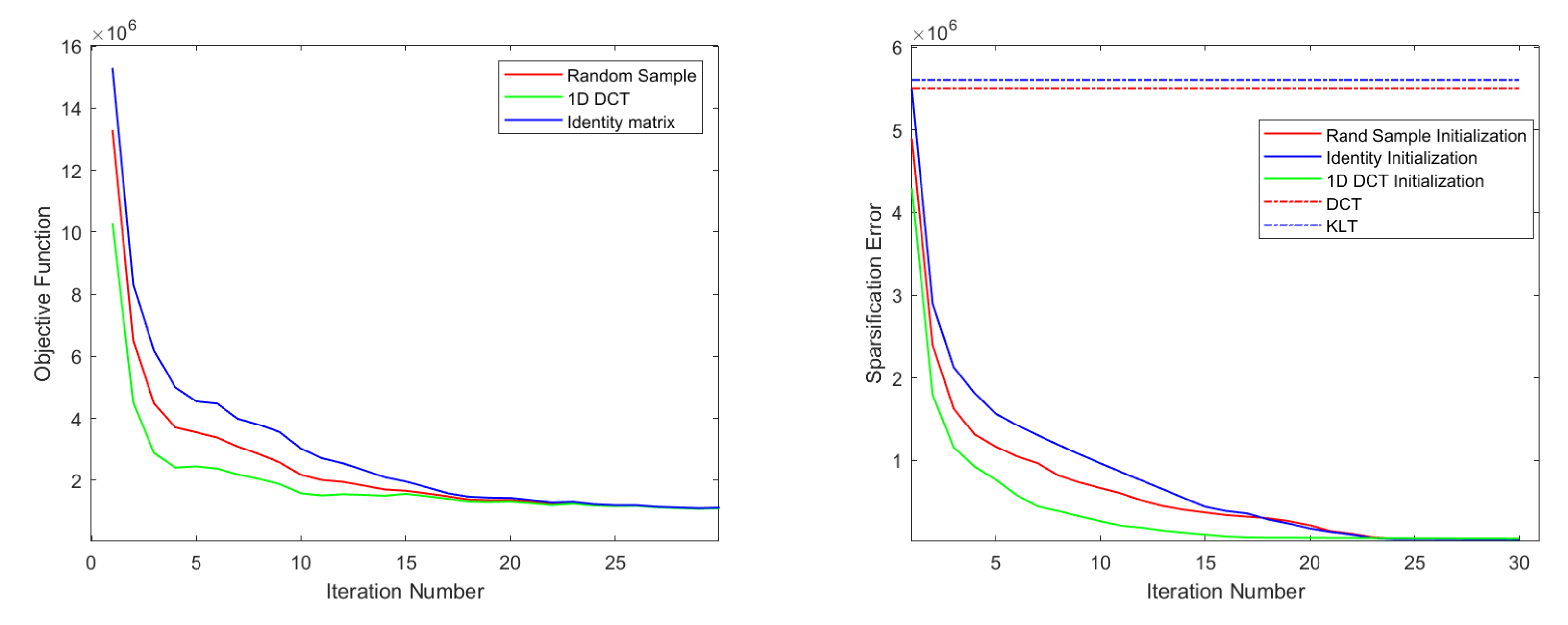
5.1. Robustness Analysis

In this subsection, we illustrate the robustness of DRTPF by training DRTPF using the image ’Barbara’ and testing DRTPF for denoising the same image with Gaussian white noise added. The noise level (standard deviation) $\delta$ ranged from 20 to 60 with a step size of 2. In the experiment, the frames $\mathbf{\Phi }$ and $\mathbf{\Psi }$ of size $100\times 200$ were initialized as 1D overcomplete DCT (ODCT) and $10\times 10$ overlapping mean-subtracted patches were used. The patch size was set as $8\times 8$ with stripe 1. We set the parameters ${\eta }_1=1.1$ and ${\eta }_3=1e+7$, and ${\eta }_2$ was replaced by the ${\ell }_0$ thresholding $0.6\sigma$ (i.e., ${\parallel \mathbf{Y}\parallel }_0\le 0.6\sigma$). For comparison, our proposed algorithm was compared with K-SVD [14]. The size of dictionary learnt from K-SVD is $8\times 256$ at its optimal state, according to the previous work.

We show the denoising result in Figure 1, from which it is apparent that with higher noise, our DRTPF method outperformed K-SVD more and more. In other words, our proposed model has good robustness. In fact, in our model, the sparse coefficients are calculated accurately by the inner product of the signals and the frame $\mathbf{\Psi }$, and are limited to a certain range. Theoretically, it should be more robust. The learnt transforms $\mathbf{\Phi }$ and $\mathbf{\Psi }$ are illustrated in Figure 2. These figures show that our frame learning method can capture the features in both analysis and synthesis ways. Figure 3 shows two exemplified visual results on the images ‘Babara’ at noise level $\sigma =30$ and $\sigma =50$. From Figure 3 we know that our proposed DRTPF can obtain more clearer features than K-SVD [14].

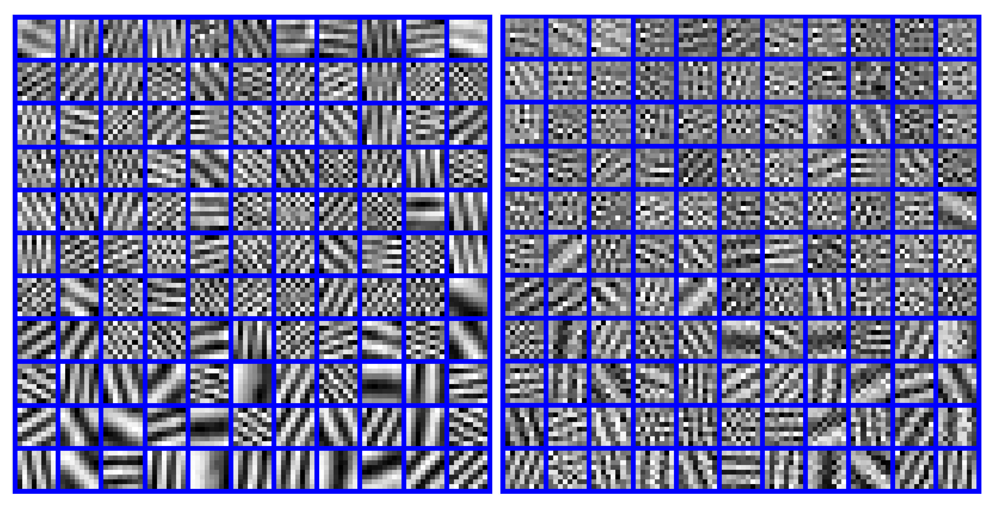
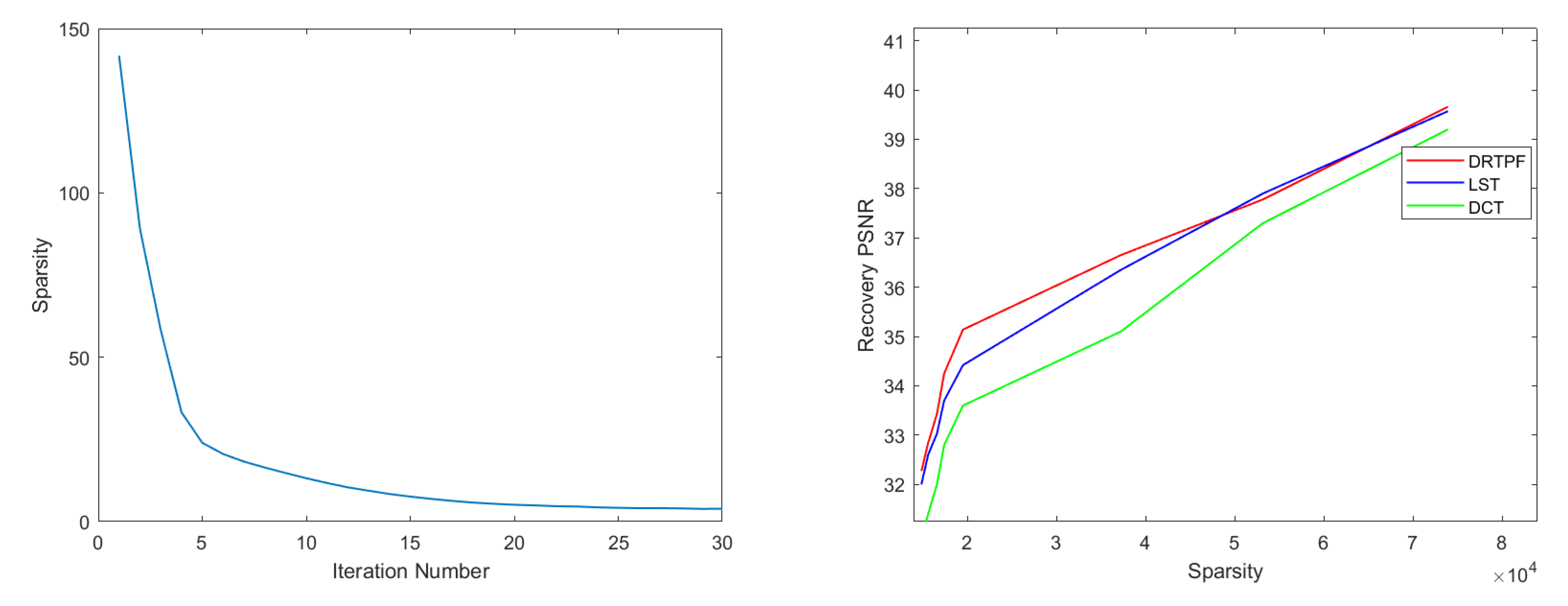
5.2. Sparsification of Nature Images

A classic sparsifying transform learning model [21] is formulated as

$$\begin{array}{cc}\hfill & \underset{\mathbf{W},\mathbf{Y}}{min}{\parallel \mathbf{W}\mathbf{X}-\mathbf{Y}\parallel }_F^2-\lambda logdet\mathbf{W}+\mu {\parallel \mathbf{W}\parallel }_F^2\hfill \\ \hfill & \mathrm{s}.\mathrm{t}.\parallel {\mathbf{Y}}_i{\parallel }_0\le s\forall i,\hfill \end{array}$$

(28)

where $\mathbf{X}$ is the training data, $\mathbf{Y}$ are the sparse coefficients, and $\mathbf{W}$ is the learnt transform. The quality of the learnt transforms in the experiment [21] was judged based on their condition number and sparsification error. Similar to the experimental setting in [21], we also evaluated the effectiveness of the transforms learnt from our DRTPF by their condition number and sparsification error. The ${\mathbf{l}}_2$-norm condition number of the transform operator $\mathbf{\Phi }$ is denoted as the ratio of the maximum singular value to the minimum singular value of $\mathbf{\Phi }$; that is,

$${\mathcal{K}}_{\mathbf{\Phi }}=\frac{{\delta }_{max}\left(\mathbf{\Phi }\right)}{{\delta }_{min}\left(\mathbf{\Phi }\right)}.$$

(29)

In our case, the condition number ${\mathcal{K}}_{\mathbf{\Phi }}=1$, as the maximum and minimum singular values (which are determined by the optimal frame bounds) must be equal to 1. Similarly, we can obtain that ${\mathcal{K}}_{\mathbf{\Psi }}=1$. It is the best case when the transform operators have condition number equal to 1. The sparsification error of the model (28) is defined as

$$SE={\parallel \mathbf{WX}-\mathbf{Y}\parallel }_F^2.$$

(30)

Similarly, we define the ‘sparsification error’ of the proposed DRTPF, to measure the energy loss due to sparse representation, which is formulated as

$$\widetilde{SE}={\parallel \mathbf{Y}-{\mathcal{S}}_{\mathit{\lambda }}\left({\mathbf{\Psi }}^T\mathbf{X}\right)\parallel }_F^2.$$

(31)

The ‘sparsification error’ indicates the compact ability of the transform $\mathbf{\Psi }$ with reasonable ignorance of the thresholding operator ${\mathcal{S}}_{\lambda }(·)$.

To demonstrate that our model and algorithms are insensitive to the initialized transforms, we applied the proposed sparse coding and transform operator pair learning algorithms to train a pair of transforms. The training data are patches of size $10\times 10$ extracted from the image ‘Babara’ which is shown in Figure 4. The trained transform pair are of size $100\times 200$. We extracted the patches with non-overlap and removed the DC values of every sample. We set the parameters ${\eta }_1=1.1$ and ${\eta }_3=1e+7$, and ${\eta }_2$ was replaced by the ${\ell }_0$ thresholding $0.6\sigma$, as before. The matrices used for initialization were the 1D DCT matrix, the matrix with random columns sampled from the training data, and the redundant identity matrix. As the transform for DRTPF is redundant, the redundandt identity matrix here is formed as $\left[\mathbf{I}\mathbf{I}\right]$ where $\mathbf{I}$ is the identity matrix of size $100\times 100$.

The convergence curve of the objective function and the ‘sparsification error’ are shown in Figure 5. From the left sub-figure of Figure 5 we know that our proposed algorithm for DRTPF is converged, and all the initializations converge to the same result after about 20 iterations which demonstrate that our proposed DRTPF and the corresponding algorithm are insensitive to different initializations. The right sub-figure of Figure 5 shows the ‘sparsification error’ of the three initialized methods, the 2D DCT transform of and the KLT transform. The 2D DCT is formed by the Kronecker product of two 1D DCT transform, i.e., $\mathbf{D}={\mathbf{D}}_0\otimes {\mathbf{D}}_0$, where ${\mathbf{D}}_0$ is the 1D DCT transform of size $8\times 8$ and ⊗ denotes the Kronecker product. The KLT transform $\mathbf{K}$ of size $64\times 64$ is obtained by principle component analysis (PCA) method. The ‘sparsification error’ of 2D DCT and KLT are calculated via the model in [21] at iteration zero. This figure shows that the ‘sparsification error’ of the proposed DRTPF model is also converged and insensitive to the initialization matrices. In fact, the loss function of the proposed DRTPF mainly contains two partions: ${\parallel \mathbf{X}-\mathbf{\Phi }\mathbf{Y}\parallel }_F^2$ and $\parallel \mathbf{Y}-{\mathcal{S}}_{\mathit{\lambda }}\left({\mathbf{\Psi }}^T\mathbf{X}\right){\parallel }_F^2$. The first partion is the recovery loss (i.e., the loss in temporal domain) and the second partion is the ‘sparsification error’ (i.e., the loss in frequency domain). Our proposed model aims to achieve low error both in temporal domain and frequency domain.

To illustrate the behavior of the proposed DRTPF in image representation, we choose six images shown in Figure 4 to train transforms and recover images. The Figure 6 shows the average sparsity curve and the recovery PSNR values with the increase of the sparsity. From the left sub-figure we know that the images are well sparsified along the iterative process. This figure is generated by setting $\parallel {\mathbf{y}}_i{\parallel }_0<5$ and the recovery PSNR is 32.27 dB. For each sample ${\mathbf{x}}_i$ vectorized by a $10\times 10$ patch, its correspondinge sparse coefficients ${\mathbf{y}}_i$ is of length 200. It is easy to know that the sparsity rate is lower than $2.5\%$. Furthermore, less than $5\%$ of the data need to be stored to recover an image with PSNR larger than 32.27 dB. The right sub-figure of Figure 6 shows the average recovery PSNR values with the increase of the sparsity which is a main measurement for the quality of the learnt transform. From the figure we know that in most of the case, our proposed DRTPF can obtain a better image quality in terms of PSNR with lower sparsity than the compared LST [21] method and the classic DCT transform. The ransform for LST [21] method and the classic DCT transform are of size $64\times 64$. The transform of LST [21] is trained by 4096 $8\times 8$ samples extracted from every image shown in Figure 6 with the main of the patches removed. The experiment is set as them illustrated in the paper [21]. When the total sparsity of a $512\times 512$ image is more than 47,000, the recovery results of the proposed DRTPF and the LST [21] are nearly the same. The recovery PSNR at sparsity 47,000 is 37.3 dB.

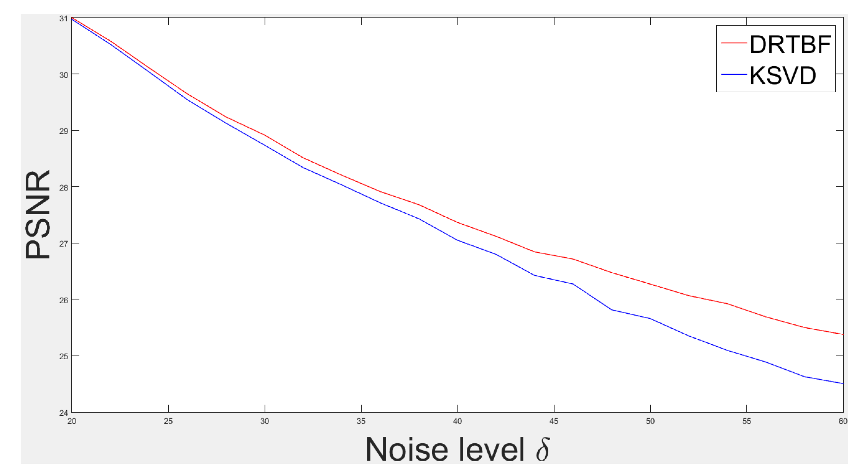
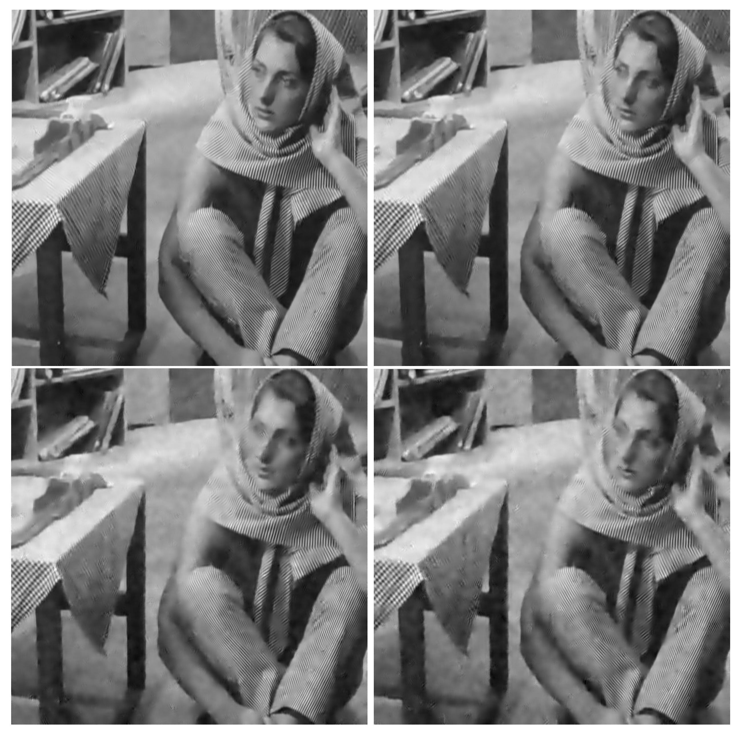
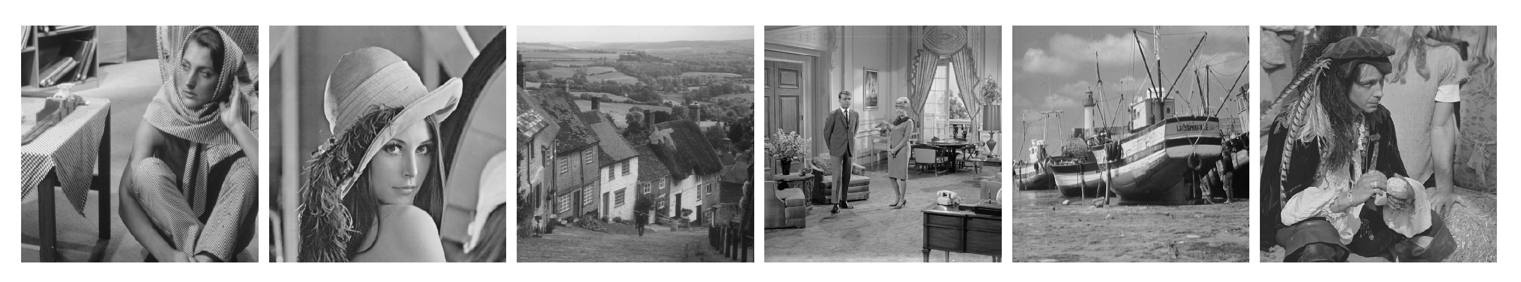
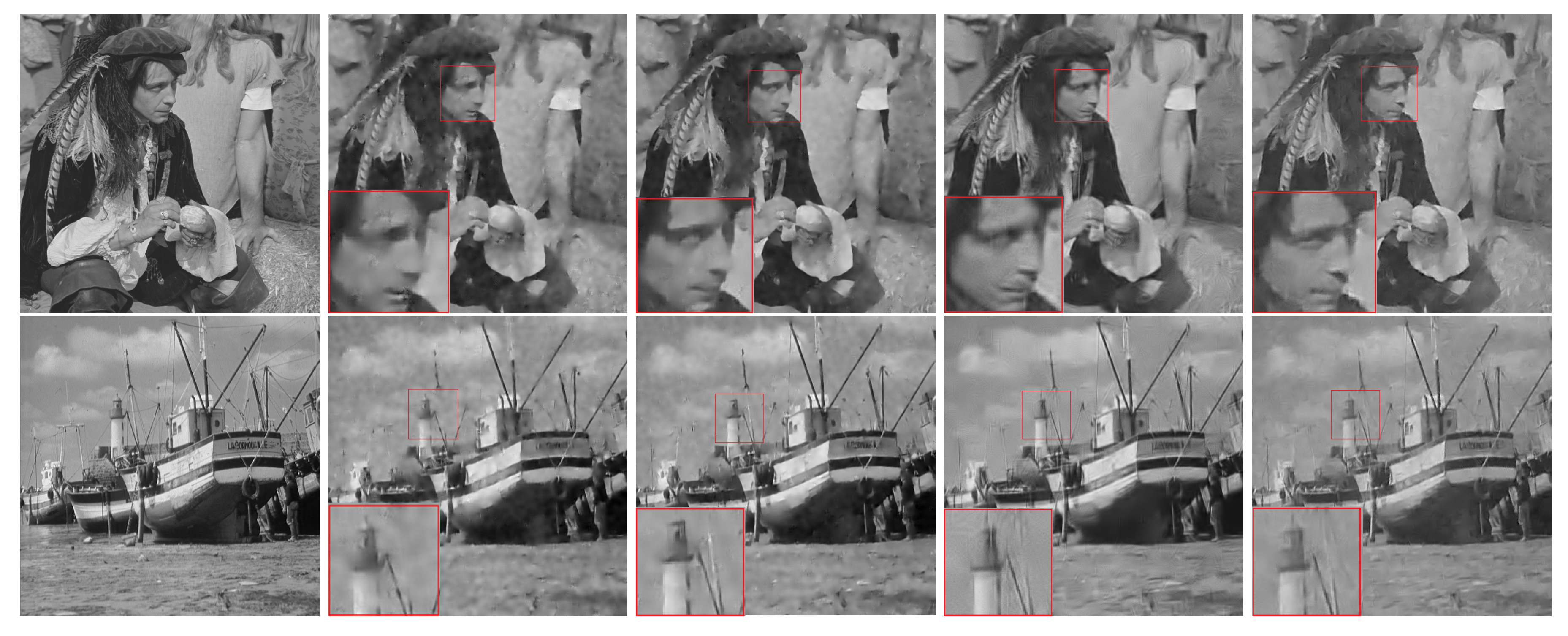
5.3. Image Denoising

In this subsection, we evaluate the performance of our DRTPF model using six natural images of size $512\times 512$, which are shown in Figure 4. We added Gaussian white noise to these images at different noise levels ($\sigma =20,30,40,50,60$). We set the parameters ${\eta }_1=1.1$ and ${\eta }_3=1e+7$, and ${\eta }_2$ was replaced by the ${\ell }_0$ thresholding $0.6\sigma$, as before. We compared DRTPF with the three most related methods of sparse representation: K-SVD [14], the overcomplete transform (T.KSVD) [3], the learning-based frame (DTF [33]), the BM3D [35] and WNNM [36]. The BM3D and WNNM are nonlocal-based methods with the parameters setting as in corresponding paper. We note that DTF works on filters, instead of image patches. In the experiment, our DRTPF method and K-SVD were the same as in Section 5.1. All methods were trained iteratively (25 times). The DTF method was initialized by 64 3-level Harr wavelet filters of size $16\times 16$. The operator size of the T.KSVD method was $128\times 64$ and the patch size it worked on was $8\times 8$ overlapping mean-subtracted patches. The hard thresholding was $s=30$.

Table 1. Average PSNR results of different noise levels on six images.

$\mathit{\sigma }$	Image	Barbara	Boat	Couple	Hill	Lena	Man	Average
20	K-SVD [14]	31.01	30.50	30.15	30.27	32.51	30.26	30.78
	T.KSVD [3]	30.02	29.30	29.25	29.21	31.45	29.01	29.71
	DTF [33]	31.07	30.35	30.20	30.31	32.56	30.07	30.76
	SSM-NTF	31.01	30.47	30.24	30.34	32.50	30.23	30.80
	BM3D [35]	32.01	31.02	30.88	30.85	33.19	30.83	31.47
	WNNM [36]	32.31	31.09	30.92	30.94	33.18	30.84	31.55
30	K-SVD [14]	28.75	28.60	28.07	28.51	30.59	28.43	28.83
	T.KSVD [3]	27.78	27.86	27.46	27.23	29.25	27.13	27.79
	DTF [33]	29.07	28.48	28.22	28.64	30.60	28.26	28.88
	SSM-NTF	29.00	28.63	28.24	28.66	30.73	28.49	28.96
	BM3D [35]	30.12	29.22	28.95	29.23	31.40	29.04	29.66
	WNNM [36]	30.32	29.30	29.02	29.33	31.50	29.10	29.76
40	K-SVD [14]	27.03	27.23	26.54	27.23	29.13	27.17	27.39
	T.KSVD [3]	26.35	26.45	25.98	26.45	28.20	26.14	26.60
	DTF [33]	27.58	27.20	26.87	27.49	29.25	26.99	27.56
	SSM-NTF	27.50	27.39	27.00	27.56	29.35	27.34	27.69
	BM3D [35]	28.68	27.92	27.58	28.08	30.11	27.83	28.37
	WNNM [36]	28.85	27.99	27.64	28.18	30.25	27.90	28.47
50	K-SVD [14]	25.71	26.05	25.42	26.29	27.92	26.18	26.26
	T.KSVD [3]	25.10	25.56	25.03	25.89	27.01	25.40	25.67
	DTF [33]	26.45	26.15	25.84	26.63	28.15	26.09	26.55
	SSM-NTF	26.43	26.32	25.99	26.79	28.40	26.40	26.72
	BM3D [35]	27.48	26.89	26.49	27.20	29.06	26.94	27.34
	WNNM [36]	27.70	26.97	26.60	27.35	29.23	27.01	27.48
60	K-SVD [14]	24.45	25.18	24.57	25.69	27.01	25.40	25.38
	T.KSVD [3]	24.50	24.88	24.36	25.40	26.60	24.78	25.09
	DTF [33]	25.64	25.33	25.04	25.91	27.22	25.38	25.75
	SSM-NTF	25.50	25.45	25.14	26.03	27.33	25.67	25.85
	BM3D [35]	26.36	26.02	25.61	26.44	28.14	26.18	26.46
	WNNM [36]	26.59	26.12	25.74	26.60	28.33	26.26	26.61

shows the comparison results, in terms of average PSNR. As shown in Table 1, our DRTPF method and the DTF method outperformed K-SVD and T.KSVD on most images, i.e., our proposed DRTPF outperforms K-SVD for 0.47 dB and outperforms T.KSVD for 0.76 dB at noise level $\sigma =60$. This result implies that methods using frames are more robust against noise. Furthermore, the higher the noise level, the better the results of DRTPF method and the DTF method than K-SVD and T.KSVD. We can also see that our DRTPF method outperformed DTF on most of the images, especially when the noise level was very high. In fact, in our model, the sparse coefficients are calculated accurately by the inner product of the signals and the frame $\mathbf{\Psi }$, and are limited to a certain range. Theoretically, it should perform better than the compared method. Figure 7 shows two exemplified visual results on the images ‘Boat’ and ‘Man’ at noise level $\sigma =40$. The PSNR of the K-SVD, T.KSVD, DTF, and the proposed DRTPF are 27.17 dB, 26.14 dB, 26.99 dB, 27.34 dB for ‘Man’ and 27.23 dB, 26.45 dB, 27.20 dB and 27.39 dB for ‘Boat’. Our proposed DRTPF and the DTF method provide more features and higher PSNR values of the two images than K-SVD and T.KSVD. Though the DTF provides higher PSNR values than K-SVD and T.KSVD, and better visual performance, the results of this method suffer from deformation and margin smoothing as it based on filter. The proposed DRTPF shows much clearer and better visual results than the other competing methods without any deformation.

All the six methods can be classified to two categories (1) without any extra constraint, e.g., nonlocal similarity, and (2) with additional prior like nonlocal similarity. Our proposed DRTPF belongs to category (1). We would like to point out that our goal was to establish a redundant transform learning method but not focus on image denoising. Our model is plain without applying any extra prior, besides the basic sparsity characteristics of the signals. The experimental results demonstrate that our proposed models can achieve better performance than traditional sparse models in image denoising. However, the methods BM3D and WNNM are based on image nonlocal self-similarity (NSS). The NSS prior refers to the fact that for a given local patch in a natural image, one can find many similar patches to it across the image. Intuitively, by stacking nonlocal similar patch vectors into a matrix, this matrix should be a low-rank matrix and have sparse singular values. The exploitation of NSS has been used to significantly boost image denoising performance. We have not involved this prior into our model.

6. Conclusions

In this paper, we propose a Parseval frame-based data-driven overcomplete transform (DRTPF) to capture features of images. We also propose the corresponding formulations, as well as algorithms for calculating the sparse coefficients and DRTPF model learning. We have proposed a general frame learning method without imposing any structure on the frame. By applying frames to redundant transforms, we combine the ideas of analysis and synthesis sparse models and let them share almost identical sparse coefficients. We conducted robustness analysis, sparsification of nature image and image denoising experiments, which demonstrated that DRTPF can outperform state-of-the-art models, as it exploits the underlying sparsity of natural signals by the integration of frames and sparse models.

In future work, we shall consider more efficient optimization algorithms for DRTPF, which facilitate the representation ability and application of the proposed method.

References

1. Marcellin, M.W.; Gormish, M.J.; Bilgin, A.B.; Boliek, M.P. An overview of jpeg-2000. In Proceedings of the DCC 2000. Data Compression Conference, Snowbird, UT, USA, 28–30 March 2000; pp. 523–541. [Google Scholar]
2. Patel, K.; Kurian, N.; George, V. Time Frequency Analysis: A Sparse S Transform Approach. In Proceedings of the 2016 International Symposium on Intelligent Signal Processing and Communication Systems (ISPACS), Phuket, Thailand, 24–27 October 2016. [Google Scholar]
3. Eksioglu, M.; Bayir, O. K-SVD Meets Transform Learning: Transform K-SVD. IEEE Signal Process. Lett. 2014, 21, 347–351. [Google Scholar] [CrossRef]
4. Ravishankar, S.; Bresler, Y. Learning Sparsifying Transforms For Image Processing. In Proceedings of the 19th IEEE International Conference on Image Processing, Orlando, FL, USA, 30 September–3 October 2012. [Google Scholar]
5. Ravishankar, S.; Bresler, Y. Learning Doubly Sarse Transforms for Image Representation. In Proceedings of the 19th IEEE International Conference on Image Processing, Orlando, FL, USA, 30 September–3 October 2012. [Google Scholar]
6. Mallat, S.; Lepennec, E. Sparse geometric image representation with bandelets. IEEE Trans. Image Process 2005, 14, 423–438. [Google Scholar]
7. Elad, M.; Aharon, M. Image denoising via sparse and redundant representations over learned dictionaries. IEEE Trans. Image Process 2006, 15, 3736–3745. [Google Scholar] [CrossRef]
8. Dong, W.; Zhang, L.; Shi, G.; Li, X. Nonlocally Centralized Sparse Representation for Image Restoration. IEEE Trans. Image Process 2013, 22, 1620–1630. [Google Scholar] [CrossRef] [PubMed] [Green Version]
9. Qi, N.; Shi, Y.; Sun, X.; Yin, B. TenSR: Multi-dimensional Tensor Sparse Representation. In Proceedings of the 2016 IEEE Conference on Computer Vision and Pattern Recognition (CVPR), Las Vegas, NV, USA, 26 June–1 July 2016; pp. 5916–5925. [Google Scholar]
10. Mairal, J.; Bach, F.; Ponce, J.; Sapiro, G.; Zisserman, A. Non-local sparse models for image restoration. In Proceedings of the 2009 IEEE 12th International Conference on Computer Vision, Kyoto, Japan, 29 September–2 October 2009; pp. 2272–2279. [Google Scholar]
11. Wang, S.; Zhang, D.; Liang, Y.; Pan, Q. Semi-Coupled Dictionary Learning with Applications to Image Super-Resolution and Photo-Sketch Synthesis. In Proceedings of the 2012 IEEE Conference on Computer Vision and Pattern Recognition, Providence, RI, USA, 16–21 June 2012; pp. 2216–2223. [Google Scholar]
12. Yang, J.; Wang, Z.; Lin, Z.; Cohen, S.; Huang, T. Coupled dictionary training for image super-resolution. IEEE Trans. Image Process 2012, 21, 3467–3478. [Google Scholar] [CrossRef] [PubMed]
13. Yang, J.; Wright, J.; Huang, T.; Ma, Y. Image superresolution via sparse representation. IEEE Trans. Image Process 2010, 19, 2861–2873. [Google Scholar] [CrossRef] [PubMed]
14. Aharon, M.; Elad, M.; Bruckstein, A. K-SVD: An algorithm for designing overcomplete dictionaries for sparse representation. IEEE Trans. Signal Process 2006, 54, 4311–4322. [Google Scholar] [CrossRef]
15. Skretting, K.; Engan, K. Recursive least squares dictionary learning algorithm. IEEE Trans. Signal Process 2010, 58, 2121–2130. [Google Scholar] [CrossRef]
16. Yaghoobi, M.; Nam, S.; Gribonval, R.; Davies, M.E. Noise aware analysis operator learning for approximately cosparse signals. In Proceedings of the 2012 IEEE International Conference on Acoustics, Speech and Signal Processing (ICASSP), Kyoto, Japan, 25–30 March 2012; pp. 5409–5412. [Google Scholar]
17. Ophir, B.; Elad, M.; Bertin, N.; Plumbley, M. Sequential minimal eigenvalues—An approach to analysis dictionary learning. In Proceedings of the 2011 19th European Signal Processing Conference, Barcelona, Spain, 29 August–2 September 2011; pp. 1465–1469. [Google Scholar]
18. Rubinstein, R.; Peleg, T.; Elad, M. Analysis K-SVD: A Dictionary-Learning Algorithm for the Analysis Sparse Model. IEEE Trans. Signal Process. 2012, 61, 661–677. [Google Scholar] [CrossRef] [Green Version]
19. Rubinstein, R.; Faktor, T.; Elad, M. K-SVD dictionary-learning for the analysis sparse model. In Proceedings of the 2012 IEEE International Conference on Acoustics, Speech and Signal Processing (ICASSP), Kyoto, Japan, 25–30 March 2012; pp. 5405–5408. [Google Scholar]
20. Wen, B.; Ravishankar, S.; Bresler, Y. Learning Overcomplete Sparsifying Transforms With Block Cosparsity. In Proceedings of the ICIP, Paris, France, 27–30 October 2014. [Google Scholar]
21. Ravishankar, S.; Bresler, Y. Learning Sparsifying Transforms. IEEE Trans. Signal Process. 2013, 61, 1072–1086. [Google Scholar] [CrossRef]
22. Parekh, A.; Selesnick, W. Convex Denoising using Non-Convex Tight Frame Regularization. IEEE Signal Process. Lett. 2015, 22, 1786–1790. [Google Scholar] [CrossRef] [Green Version]
23. Lin, J.; Li, S. Sparse recovery with coherent tight frames via analysis Dantzig selector and analysis LASSO. Appl. Comput. Harmon. Anal. 2014, 37, 126–139. [Google Scholar] [CrossRef]
24. Liu, Y.; Zhan, Z.; Cai, J.; Guo, D.; Chen, Z.; Qu, X. Projected Iterative Soft-Thresholding Algorithm for Tight Frames in Compressed Sensing Magnetic Resonance Imaging. IEEE Trans. Med. Image 2016, 35, 2130–2140. [Google Scholar] [CrossRef] [PubMed] [Green Version]
25. Chan, H.; Riemenschneider, D.; Shen, L.; Shen, A.Z. Tight frame: An efficient way for high-resolution image reconstruction. Appl. Comput. Anal. 2004, 17, 91–115. [Google Scholar] [CrossRef] [Green Version]
26. Ron, A.; Shen, Z. Affine system in L2(Rd): The analysis of the analysis operator. J. Funct. Anal. 2013, 148, 408–447. [Google Scholar] [CrossRef] [Green Version]
27. Candes, E. Ridgelets: Estimating with ridge functions. Ann. Statist. 1999, 31, 1561–1599. [Google Scholar] [CrossRef]
28. Candes, E.J.; Donoho, D.L. Recovering edges in ill-posed inverse problems: Optimality of curvelet frames. Ann. Statist. 2002, 30, 784–842. [Google Scholar] [CrossRef]
29. Kutyniok, G.; Labate, D. Construction of regular and irregular shearlet frames. J. Wavelet Theory Appl. 2007, 1, 1–10. [Google Scholar]
30. Casazza, P.G.; Kutyniok, G.; Philipp, A.F. Introduction to Finite Frame Theory. In Finite Frames; Birkhäuser: Boston, MA, USA, 2012. [Google Scholar]
31. Cao, C.; Gao, X. Compressed sensing image restoration based on data-driven multi-scale tight frame. J. Comput. Appl. Math. 2017, 309, 622–629. [Google Scholar] [CrossRef]
32. Li, J.; Zhang, W.; Zhang, H.; Li, L.; Yan, A. Data driven tight frames regularization for few-view image reconstruction. In Proceedings of the 13th International Conference on Natural Computation, Fuzzy Systems and Knowledge Discovery, ICNC-FSKD 2017, Guilin, China, 29–31 July 2017; pp. 815–820. [Google Scholar]
33. Cai, J.; Ji, H.; Shen, Z.; Ye, G. Data-driven tight frame construction and image denoising. Appl. Comput. Harmon. Anal. 2014, 37, 89–105. [Google Scholar] [CrossRef]
34. Rubinstein, R.; Zibulevsky, M.; Elad, M. Efficient Implementation of the K-SVD Algorithm Using Batch Orthogonal Matching Pursuit; Technical Report CS-2008-08; Technion-Israel Institute of Technology: Haifa, Israel, 2008. [Google Scholar]
35. Katkovnik, V.; Foi, A.; Egiazarian, K.; Astola, J. From local kernel to nonlocal multiple-model image denoising. Int. J. Comput. Vis. 2010, 86, 1–32. [Google Scholar] [CrossRef] [Green Version]
36. Gu, S.; Zhang, L.; Zuo, W.; Feng, X. Weighted Nuclear Norm Minimization with Application to Image Denoising. In Proceedings of the 2014 IEEE Conference on Computer Vision and Pattern Recognition, Columbus, OH, USA, 23–28 June 2014; pp. 2862–2869. [Google Scholar]
Figure 1. Robustness Analysis. DRTPF is trained and tested using the image ‘Barbara’. The X-label is the noise level δ and the Y-label is the PSNR. It can be seen that DRTPF performs more robustly than K-SVD.
Applsci 10 02891 g001
Figure 2. The learnt operators Φ (left) and Ψ (right) for barbara.
Applsci 10 02891 g002
Figure 3. Reconstruction of barbara using DRTPF (left) and K-SVD [14] (right). Top: σ = 30 ; bottom: σ = 50 .
Applsci 10 02891 g003
Figure 4. The test images ‘Barbara’, ‘Lena’, ‘Hill’, ‘Couple’, ‘Boat’, and ‘Man’.
Applsci 10 02891 g004
Figure 5. Convergence Curve and Sparsification Error. Left: The X-label is the iteration number. Right: The Y-label is the objective function and the sparsification error, respectively. It can be seen that our DRTPF learning algorithm is convergent and insensitive to initialization.
Applsci 10 02891 g005
Figure 6. The average Sparsity and Recovery PSNR. Left: The X-label is the iteration number and the Y-label is the average sparsity. Right: The X-label is the average sparsity and the Y-label is the average Recovery PSNR.
Applsci 10 02891 g006
Figure 7. Visual comparison of reconstruction results by different methods on ‘Man’ and ‘Boat’. From left to right: original, T.KSVD [3], K-SVD [14], DFT [33], and DRTPF.
Applsci 10 02891 g007