Article

Donning/Doffing and Arm Positioning Influence in Upper Limb Adaptive Prostheses Control

1
Instituto de Telecomunicaciones y Aplicaciones Multimedia (ITEAM), Departamento de Comunicaciones, Universitat Politècnica de València, 46022 Valencia, Spain
2
Instituto Universitario de Automática e Informática Industrial, Departamento de Ingeniería de Sistemas y Automática, Universitat Politècnica de València, 46022 Valencia, Spain
*
Author to whom correspondence should be addressed.
Appl. Sci. 2020, 10(8), 2892; https://doi.org/10.3390/app10082892
Submission received: 29 February 2020 / Revised: 17 April 2020 / Accepted: 20 April 2020 / Published: 22 April 2020
(This article belongs to the Section Applied Biosciences and Bioengineering)

Abstract

:
New upper limb prostheses controllers are continuously being proposed in the literature. However, most of the prostheses commonly used in the real world are based on very old basic controllers. One reason to explain this reluctance to change is the lack of robustness. Traditional controllers have been validated by many users and years, so the introduction of a new controller paradigm requires a lot of strong evidence of a robust behavior. In this work, we approach the robustness against donning/doffing and arm position for recently proposed linear filter adaptive controllers based on myoelectric signals. The adaptive approach allows to introduce some feedback in a natural way in real time in the human-machine collaboration, so it is not so sensitive to input signals changes due to donning/doffing and arm movements. The average completion rate and path efficiency obtained for eight able-bodied subjects donning/doffing five times in four days is 95.83% and 84.19%, respectively, and for four participants using different arm positions is 93.84% and 88.77%, with no statistically significant difference in the results obtained for the different conditions. All these characteristics make the adaptive linear regression a potential candidate for future real world prostheses controllers.

1. Introduction

In spite of the continuous improvement in the amputation rehabilitation and prosthetic restoration [1], living without a limb limits the daily life activities leading to a lower quality of life. Many people in the world suffer from the loss of a limb. As an example, Ziegler-Graham et al. estimated that 1.6 million people in the USA were suffering this situation in 2005 and predicted to double this number by 2050 [2]. Upper limb amputation is the removal of any part of the arm or forearm. Amputations at or above the wrist are considered as a major one, being the most common case the amputation at the transradial level. In the same study [2], 540,000 people living in the USA were estimated to have an upper limb loss, of which around 40,000 correspond to amputations above the wrist.
In the last years the upper limb prostheses control has become a growing research field [3]. The prosthetic industry has been developing new prostheses to mitigate the effects of losing a limb. However, despite of all the research and efforts carried out, there is a gap between the newer developments in the academia and the available commercial prostheses. The main problems the research faced have been a low user satisfaction and high prosthesis rejection due to a non-functional use [4,5,6,7,8]. Because of that, nowadays a primary goal in this field is to find prostheses control protocols robust enough to be used in real life.
Different biosignals can be used as inputs for the control system. Electromyography (EMG), the measurement of superficial electric potentials during muscle contractions, is the most established input source for predicting the user’s intent. Its easy access and processing makes EMG a better option than other input sources such as electroencephalogram (EEG). EMG signals allow to infer the neuromuscular activity information sent to perform a specific movement. Multiple studies show the good performance of EMG signals to predict the user’s intent [9,10,11,12,13,14,15,16,17]. The control system extracts the most important information from the data and maps it into a feature space. The extracted features are used to train an algorithm that learns to predict the user’s intent. This output is presented to the user through some feedback channel, and the whole system is tested in unknown situations. During the last years, there have been developments in all processes of the control loop: new features and feature extraction methods [18,19], new algorithms based on classification [20,21,22] and regression models [23,24], new feedback procedures [25,26,27,28,29,30,31] and new prostheses technology [32]. Nevertheless, most of these improvements have never been implemented in real life devices. One of the reasons is the lack of usability in real world scenarios. Thus, although these new systems have a high performance in controlled environments, they exhibited a lack of robustness when tested in daily life situations on realistic environments [3,9,33]. Several factors could generate non-stationarities in the EMG signals that fed the system limiting a robust performance. The most common problems are: limitations of EMG signal acquisition process [34,35,36,37], arm positioning [38,39], electrode shifting [39,40,41], skin conditions [25], fatigue [42] or time degradation [43]. These factors affected the reliability of modern prosthesis control methods over time and conditions of use. A lot of work is being done in this direction in order to obtain controllers that behave in a more natural and robust way [44,45,46,47,48].
We have previously proposed an adaptive auto-regressive proportional myoelectric control system [49], which showed a much effective performance in controlled environments, such as laboratory experiments, than today’s state of the art regression models. The goal in this new work is to analyze whether this higher performance is maintained under real life “noisy” conditions, i.e., to study the robustness of the system against external disturbances while performing the virtual task. Firstly, we analyze the effect of time degradation and small electrode shifting; to do this, the participants simulate the real life use of prostheses by a donning/doffing experiment during a four-day period. Secondly, we study the robustness and generalization of the model for different configuration environments; to do this, the participants carried out a consecutive series of tasks while the arm position is changing. Our results demonstrate the algorithm capabilities to overcome non-stationary inputs without any re-adjustment. These capabilities are essential for a comfortable real prosthesis control and open the possibility that the proposed method could be implemented in the future in a test stage with real patients in a clinically supervised experiment.

2. Materials and Methods

2.1. Data Acquisition

A Myo Armband from Thalmics was used for the data acquisition process. The sensor is a flexible hardware that can be used in upper limbs with 7.5 to 13 inches forearm circumference. It includes 8 bipolar EMG electrodes sampling at 200 Hz with an 8 bit resolution. With these specifications, simple signal amplitude features are obtainable. A Bluetooth connection is opened to send the data and process it in a MATLAB environment. We used MATLAB 16a 64 version running on a 2.6 GHz personal laptop with 8 GB RAM. The Myo Armband was always placed in the right forearm of the participant, as in Figure 1, in the same location and orientation for all participants (LED light of the sensor pointing to the hand).
This experimentation would be reproducible in patients with limb deficiencies with a stump of at least 3 inches from the elbow to place the armband. In our previous work [49], the system was used in amputees that satisfied that specification. The armband is placed to measure the superficial EMG of the flexor carpi radialis and ulnaris muscles, extensor carpi radialis longus and the brachioradialis muscle, among other residual EMG measurements. In that paper the experiment was only conducted with forearm EMG activity so there are no evidences for EMG signals obtained from other muscles.
The feature used as the input vector x ( t ) is the moving root mean square (RMS) of the digitized EMG signals x ^ ( t ) :
x ( t ) = 1 N k = t 1 t x ^ 2 ( k )
where t 1 = t N + 1 , x ^ ( k ) R 8 × 1 is the eight dimensions digitized muscular activity, and N is the sample size. This is the discrete version counterpart of the continuous moving RMS value:
x ( τ ) = 1 T τ T τ x ^ 2 ( t ) d t
where N = T · f s and f s is the sampling frequency. In our case, f s = 200 Hz, T = 200 ms and N = 40 . A new feature vector is calculated every 40 ms, resulting in a 25 Hz feature rate with 160 ms overlapping between consecutive input vectors.
The two studies were conducted independently with different participants, so we can guarantee that there was no learning contamination from one experiment to the other; 8 able-bodied participants (5 males and 3 females) executed the donning/doffing experiment and 4 participants (2 males and 2 female) the arm position experiment. Participants were in between 20–50 years old. All individuals provided written informed consent before the experiment. The experiments were performed in accordance with the declaration of Helsinki and were approved by the UPV ethics committee, approval number P11-23-03-18.

2.2. Method

Our model controlled two independent degrees of freedom (DoF). Since we used a regression model, all movements (single DoF activation or combined) were allowed at any time instead of the classical classification approaches where the input signals are mainly mapped into discrete movements [9,10,20,21,22,50]. In this scenario, both degrees of freedom correlate independent movements, so we modeled each one separately. The current position is estimated based on the previous one and the myoelectric input signal generated by the user during forearm muscle contractions. Mathematically, the problem can be stated as an ARMA(1,q) linear system:
y i ( t ) = a i ( t ) y i ( t 1 ) + k = 0 q b i , k T ( t ) x ( t k ) , i = 1 , 2
where y i ( t ) , i = 1 , 2 are the current position in each direction, y i ( t 1 ) the previous ones, a i ( t ) the two feedback coefficients to be estimated, b i , k ( t ) the input signal filters that must also be estimated and x ( t ) the input signals, i.e., the RMS feature vector obtained from the myoelectric activity using Equation (1).
The order q of the FIR filter must be chosen according to the sampling frequency and the signal to noise level. In this study, we used the simplified equation where the input has no memory, i.e., q = 0 , since the signals have enough power and the reaction time between the visual stimulus and the muscular response is almost immediate [51]. Assuming q = 0 , the final model reads:
y i ( t ) = a i ( t ) y i ( t 1 ) + j = 1 M b i , j ( t ) x j ( t ) , i = 1 , 2
where M is the number of myoelectric channels, in our case M = 8 .
The goal in Equation (4) is to obtain the coefficients a i ( t ) and the filters b i ( t ) that minimize the mean squared error between the real target position d i ( t ) and the estimated one y i ( t ) :
ε M S E ( t ) = i = 1 2 E d i ( t ) y i ( t ) 2
This is a regression problem where the system is modeled by an ARMA(1,0) filter with unknown AR part a i ( t ) and MA part b i ( t ) . The filters were learned by the algorithm during a real-time training session.
To solve Equation (4), we need an adaptive solution since it must work in real time, i.e., for each new input signal, we must obtain an estimated output position. As the actual position depends recursively on previous estimated positions, the error is a non linear function of the parameters. In [49], we presented an adaptive algorithm with a recursive Gauss–Newton updating rule. We summarize here the algorithm (see [49] for details about the derivation for the general ARMA(p,q) case). To simplify the notation, we concatenated in one column vector β ( t ) all the coefficients to be estimated. Each movement direction has one coefficients vector: β i ( t ) = [ a i ( t ) , b I , 1 ( t ) , , b i , M ( t ) ] T , i = 1 , 2 .
First, all parameters were initialized; the initial coefficients were set to zero: a 1 ( 0 ) = a 2 ( 0 ) = 0 , and b 1 ( 0 ) = b 2 ( 0 ) = [ 0 , 0 , , 0 ] T . The initial position was considered at the origin ( y 1 ( 0 ) , y 2 ( 0 ) ) = ( 0 , 0 ) , and two matrices used for the coefficients update were initialized randomly, P 1 ( 0 ) = P 2 ( 0 ) = α I , with α a small value and I the identity matrix. Two additional auxiliary filtered versions of the input x ˜ i ( t ) and output y ˜ i ( t ) signals for each movement are defined and concatenated in a column vector z ˜ i ( t ) = [ y ˜ i ( t 1 ) , x ˜ i , 1 ( t ) , , x ˜ i , M ( t ) ] T .
Each sample x ( t ) = [ x 1 ( t ) , , x M ( t ) ] T obtained as it is explained in the Data Acquisition section fed the algorithm. For each observation and direction, the following calculations were carried out:
  • Estimate the new predicted position ( y 1 ( t ) , y 2 ( t ) ) :
    y i ( t ) = a i ( t ) y i ( t 1 ) + j = 1 M b i , j ( t ) x j ( t ) , i = 1 , 2
  • Calculate the error between the real position and the estimated one for each direction:
    e i ( t ) = d i ( t ) y i ( t )
  • Update the z ˜ i ( t ) vectors filtering the output and input signals with the AR part of the model, obtaining the new signals y ˜ i ( t ) and x ˜ i , j ( t ) :
    y ˜ i ( t ) = y i ( t ) + a i ( t ) y ˜ i ( t 1 )
    x ˜ i , j ( t ) = x j ( t ) + a i ( t ) x ˜ i , j ( t ) , j = 1 , , M
    z ˜ i ( t ) = [ y ˜ i ( t 1 ) , x ˜ i , 1 ( t ) , , x ˜ i , M ( t ) ] T
  • Update the P i matrices and the model parameters:
    P i ( t + 1 ) = λ 1 P i ( t ) P i ( t ) z ˜ i ( t ) z ˜ i T ( t ) P i ( t ) λ / ( 1 λ ) + z ˜ i T ( t ) P i ( t ) z ˜ i ( t )
    β i ( t + 1 ) = β i ( t ) + μ P i ( t + 1 ) z ˜ i ( t ) e i ( t )
    where λ is a forgetting factor, typically 0.9 λ < 1 , that establishes the importance of previous observations when obtaining the new estimate. In terms of the cost function:
    ε E R L S ( T ) = t = 1 T λ T t d ( t ) y ( t ) 2
    If λ = 1 , the algorithm has an everlasting memory, and all samples are considered to estimate the present coefficients. The parameter μ is the convergence factor, and usually μ = λ .
The previous steps were run iteratively for every new input sample until the end of the training session.

2.3. Study Design

All participants were asked to sit in a pleasant position so that they could perform the entire experiment in a comfortable way, minimizing the movement of different parts of the body other than the desired arm movements. Two wrist DoFs were used in this study: wrist flexion/extension and radial/ulnar deviation measuring the forearm EMG activity of those movements. The flexion/extension movements were mapped into the vertical axis and radial/ulnar deviation into the horizontal axis of a 2D interface. To guarantee that the participant run the experiment naturally, no more instructions were given about how to move. Few additional instructions regarding the experiment and the user interface used were given. In this way, we ensured that the subject knew the objective function and understood the procedure to achieve the goal. Henceforth, the device was initialized, and the experiment started. Experimentation had two procedures: training and testing. Depending on the experiment purpose, the protocol of the procedure execution was different.

2.3.1. Training Phase

During the training, the machine and the user collaborated to achieve a common goal: minimize the error between estimation and target. The proposed co-adaptive system set both agents (machine and user) as active learners. The machine learning algorithm obtained the model coefficients grouped in the β i ( t ) vector for each direction, while the user adapted his behavior to the estimated machine output. As feedback, a visual interface was prompted to represent the machine’s performance in a natural and understandable environment for the user.
The displayed interface had several elements (Figure 2a). In the background, there was a coordinate system centered on a resting position with two axis (mapping the movements as mentioned above). These two axis represented the DoFs controlled by the algorithm. As moving elements, there was a green circle indicating the target position d ( t ) , three small circles indicating upcoming target direction, a red cross (cursor) for the current estimated position y ( t ) , and a orange arrow indicating the current direction from the cursor to the target, i.e., the error. The UI was updated every 40 ms (25 Hz), same rate as the adaptive filter (feature vector rate). Before the experiment, the participants tested the feedback system until they got familiarized with the information given by each element.
The training process consisted in 4 laps of the same trajectory. Each lap was composed by 4 movements. Starting in an initial position, the target moved until reaching the up-top position in 4 s, rebounded and came back to the center in another 4 s. Once the movement was completed, the same was repeated for the other three directions: left, down and right. A lap was completed when the 4 direction movements were conducted. One lap was 32 s long, 8 s each movement. Therefore, the complete training (4 laps) lasted 128 s. The training phase was equal for every participant independently of the experiment. The purpose of the training was to generate the model coefficients for each participant. They were requested to try to follow the target with the cursor controlled by their wrist movements.
Since we were using a velocity control model, what was being learned was the direction of the movement, with large deviations between the target and the cursor position. Therefore, we explained the subjects to keep contracting the muscles in the correct way even if the algorithm was not learning properly or there was some offset between the target and the estimated user position.

2.3.2. Test Phase

The test phase evaluates the performance of the coefficients learned during the training. With a fixed model, the participants controlled a cursor in a visual interface used as feedback.
The interface background was the same as in the training phase, but the moving objects were altered (Figure 2b). Now the targets were presented as static orange circles. The red cursor was kept removing the orange arrow, letting the user decide the direction to reach the target without external indications.
The test consisted in a total of 36 targets that covered the full space. Targets in every direction were displayed testing in untrained positions and the ability to avoid overfitting. The participant had to reach and stay in a target for two consecutive seconds before a 10 s timer expired. Once accomplished the task, the next target was displayed, and a new 10 s timer started. If the user did not achieve the task, it was considered a miss, and a new target was prompted with the corresponding new timer. The 36 targets were shown in the same random order for all participants. The user was requested to reach each target as fast and straight as possible.

2.4. Experimental Paradigm

2.4.1. Donning and Doffing Protocol

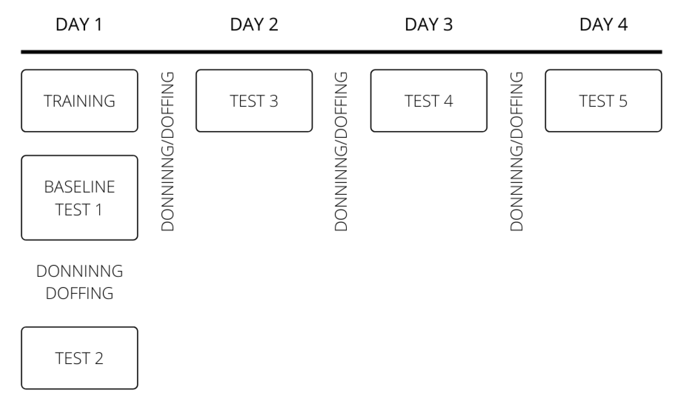
Eight participants were used to analyze the effects of donning and doffing the armband on the system performance. The right arm was set in the same position for all sessions, with the elbow flexed 90 degrees so not to add more variables. All participants executed the experimental protocol shown in Figure 3 (testing and resting days) in the same schedule to obtain comparable results.
The first day the participants completed a training phase. The model learned during the training was used in all the tests sessions in order to study its degradation through time and donning/doffing. The first test after the training was performed without any electrode shifting and without removing the sensor. This was considered the baseline test. Once the first test was completed, the Myo Armband was removed, and the participant had a 5-min break. Afterwards, a second test phase was performed relocating the Myo Armband.
The positioning was done in realistic and manual conditions without any technical procedures. The researcher photographed the initial position to place the sensor as similar as possible in further sessions. No other re-positioning considerations were taken into account trying to reproduce a realistic environment where a daily-based prosthesis user places it without absolute precision.
The following days the participants performed one test phase per day, with the same trained model, completing three more tests. At the end of the entire process, each participant had carried out one training session and five test sessions.

2.4.2. Arm Position Protocol

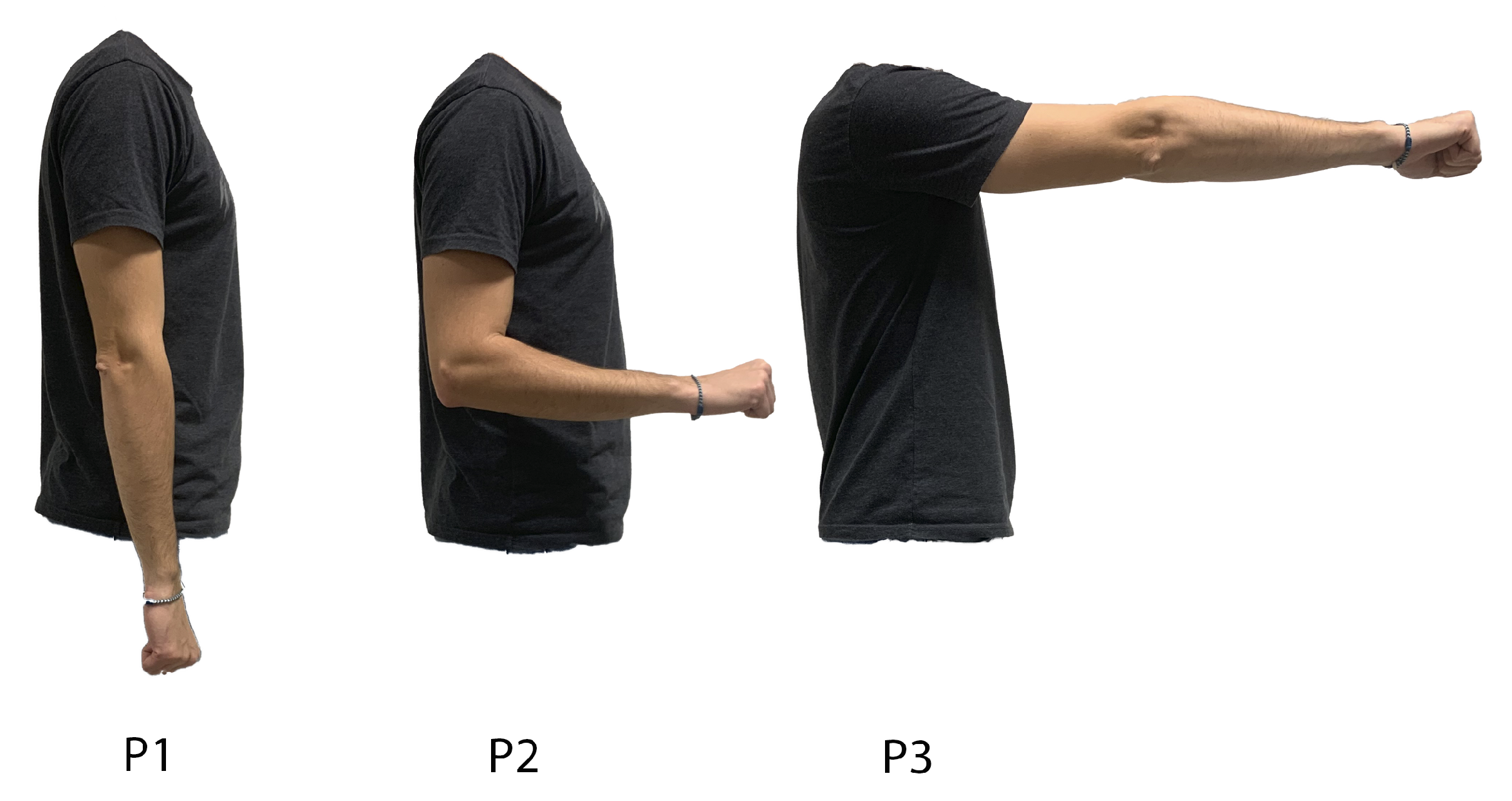
Three arm positions were adopted to analyze the effects of arm postures variation: straight arm pointing aligned with the torso (P1), elbow flexed 90 degrees (P2) and straight arm at a 90 degree angle to the torso (P3) (see Figure 4).
The experiment protocol was divided in three sessions conducted in one day. A single session had one training and four tests. First, the training was carried out in one of the three arm positions P1, P2 and P3 and then tested in all of them. The fourth test evaluates the robustness in a less controlled environment. During this test (P4), the participant was requested to variate the arm posture at his will after three consecutive targets without constrains. This was repeated two more times, until all the arm postures (P1, P2 and P3) were used as the training arm position. The test in each session using the trained position was considered the baseline to compare with the results of the other positions. The order of the training position was permuted between patients to cover all combinations.

2.5. Performance Metrics

To quantify the performance during the online test phase, we measured four quantitative metrics. The completion rate (CR) was defined as the number of hits H over the total amount of targets N expressed in a percentage scale %:
C R ( % ) = 100 · H N
We defined previously a hit such as reaching the target and staying inside for two seconds, everything in less than 10 s.
The path efficiency (PE) indicated if the distance traveled by the participant during the experiment was close to the optimal path, i.e., the shortest one. The PE was defined as the ratio in % of the sum of distances between targets and the real distance traveled by the subject:
P E ( % ) = 100 · i = 1 N d i d i 1 i = 1 N j = 1 J i y i ( j ) y i ( j 1 )
where N is the number of targets, and J i is the number of samples to get from target i to target i + 1 . For the first target i = 1 , we assumed that d 0 = ( 0 , 0 ) and y 1 ( 0 ) = ( 0 , 0 ) (the starting point for all the test experiments was the origin of coordinates). The starting point for the next segment was equal to the final position of the actual one, i.e., y i + 1 ( 0 ) = y i ( J i ) . A larger value of PE implies a more linear trajectory in the 2D space. Linear trajectories in the 2D space are directly correlated with the activation of combined DoFs movements. Therefore, the PE can be used also as an indirect measurement of the simultaneous multiple degree of freedom control.
The completion time (CT) metric measured the efficiency in the time domain. It was calculated as the time average in seconds to reach a target:
C T = i = 1 N t i N
where t i is the time in seconds to travel from target i 1 to target i. For the missed targets (the subject was not able to reach the target before 10 s and kept into the target for at least two consecutive seconds), t i = 10 in Equation (16).
To measure the stability of the system to accomplish the targets hit condition, we defined the attempt ratio (AR). It was defined as the average ratio between the number of times the subject enters the hit targets E and the number of hits H.
A R = E H
By definition, A R 1 ; the lower the AR value, the lower the attempts needed to hit the targets. A value close to 1 means that the system was very stable, since the first time that he got into the target he was able to stay for the two required seconds to be considered a hit.

3. Results

3.1. Donning and Doffing Experiment

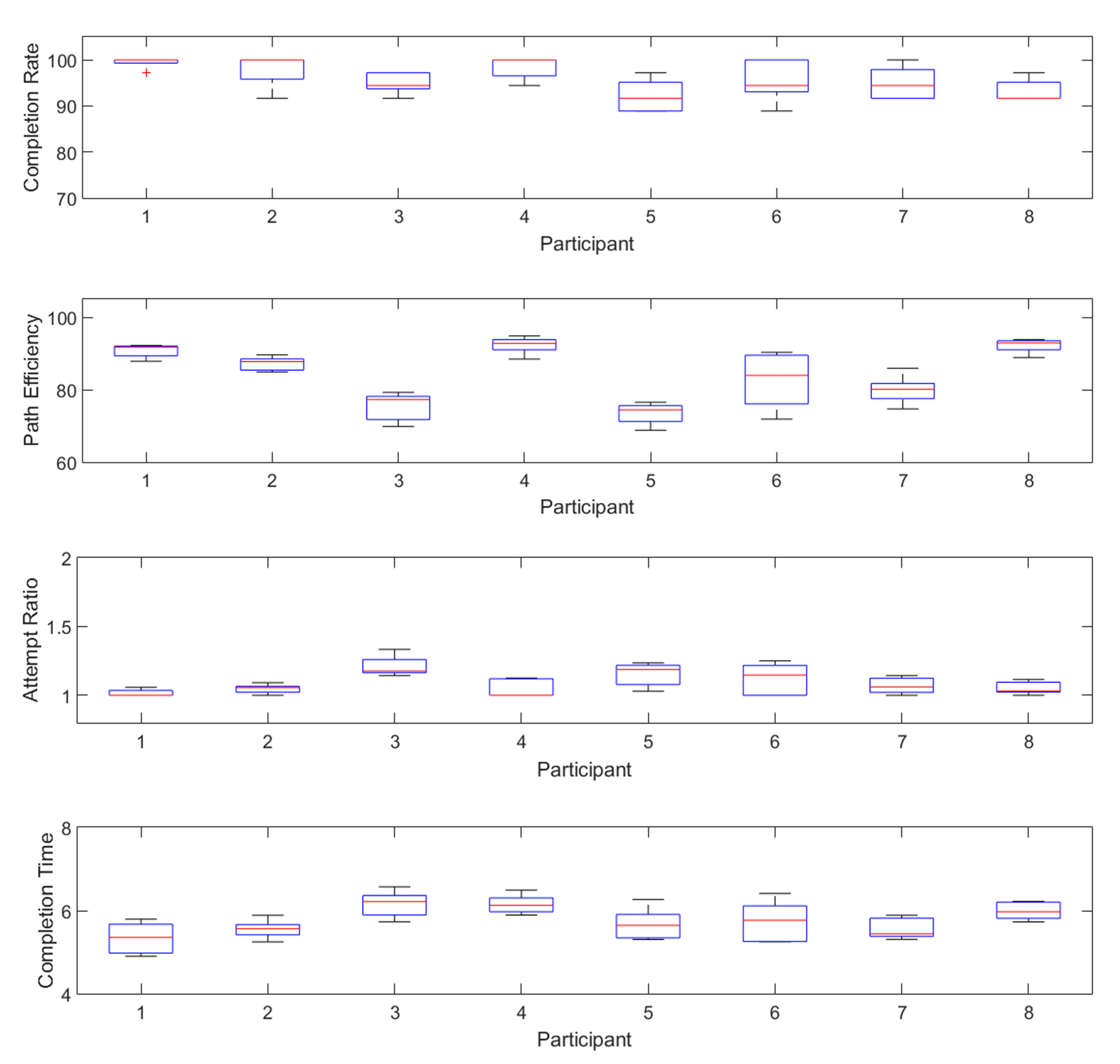
The obtained metrics (mean and variance) of the five donning/doffing experiments for each subject are shown in Table 1. They are shown graphically in a box and whisker plot in Figure 5.
Figure 5 shows that the completion rate metric had a consistent high value for all subjects. In our previous work [49], we showed that the IIR adaptive algorithm had a 95% CR when the training and test armband position were the same. In this study, it was observed that the high completion rate was not diminished by the donning/doffing effect. Three participants achieved a median 100% accuracy, and the worst result was a value of 90% for subject #3 one day. Figure 5 also shows that the variance is small for all participants and metrics. It means that after training the first day, the system was robust enough to maintain the same performance the next days both in space and time efficiency.
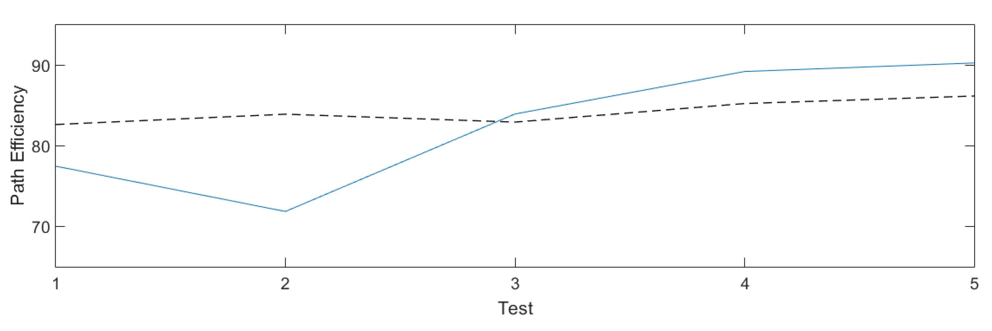
Only one participant showed a wider variance in path efficiency, subject #6. Looking into the time evolution of the results for that subject, we discovered a continuous learning trend during the experiment. This was the only patient that showed an accentuated learning behavior as the others kept a more robust performance.
Analyzing our results in depth, Figure 6 shows the PE for subject #6 (blue line) compared to the average value of all participants (black line) vs. the test number. It reveals that the PE performance of subject #6 improved during the training sessions, while the other participants had a steady performance, with an approximately 84% PE value. Thus, his higher variance in the PE metric is not due to a lack of robustness but to a learning process.
A repeated measures ANOVA ( p < 0.05 ) confirms that not one metric was changing with time, reassuring the robustness of the initial training: CR p = 0.8397 , PE p = 0.3152 , AR p = 0.8096 and CT p = 0.5311 . To confirm the robust behavior, we run a MANOVA test that restates the results obtained with the previous ANOVA analysis: There was not statistically sufficient evidence to reject the hypothesis that all metrics come from the same distribution ( p < 0.05 ).
The values in Figure 5 and Table 1 provide a visual and quantitative performance analysis of the adaptive filtering algorithm in donning/doffing experiments but do not show the dynamics of the experiments, i.e., the user experience.
To show this behavior in a more intuitive and visual way, we included some videos where the dynamics of the system are appreciated. We show the trajectories for each test for the five tests for the first seven participants in https://youtu.be/whB_6Ci76oM (participant 1), https://youtu.be/2GKl48cotCI (participant 2), https://youtu.be/iFlcD628Wnw (participant 3), https://youtu.be/DzmafnQnKcQ (participant 4), https://youtu.be/5T5EtZtTOWA (participant 5), https://youtu.be/DE5Tv4Euikc (participant 6) and https://youtu.be/Yj2aICLStl0 (participant 7). In the videos, every test is represented by a different color: red, green, blue, cyan and magenta for test 1, 2, 3, 4 and 5, respectively. The next target for a corresponding test is displayed with the same color code at any given time. For a visual purpose, targets are plotted as circles with different diameters. Note that in the real experiments all the circles (targets) had the same size. In addition, to avoid that the plots become too cumbersome because cross crossing trajectories, only a few samples are plotted. Analyzing the videos, if lines are far away, it means that some target was missed or the path efficiency was changing from test to test. The way to check the simplicity from the user point of view is to check if the trajectories are close to the straight lines joining the previous and next target. A curve that is moving around a target means that the attempt ratio was poor (AR much greater than 1), since it means that the user was entering and leaving the target in an unstable way. This behavior of the system will be translated from the user point of view, first, as an insecure experience, and later, if he finds out that this instability is persistent in time, in a disaffection to the system.
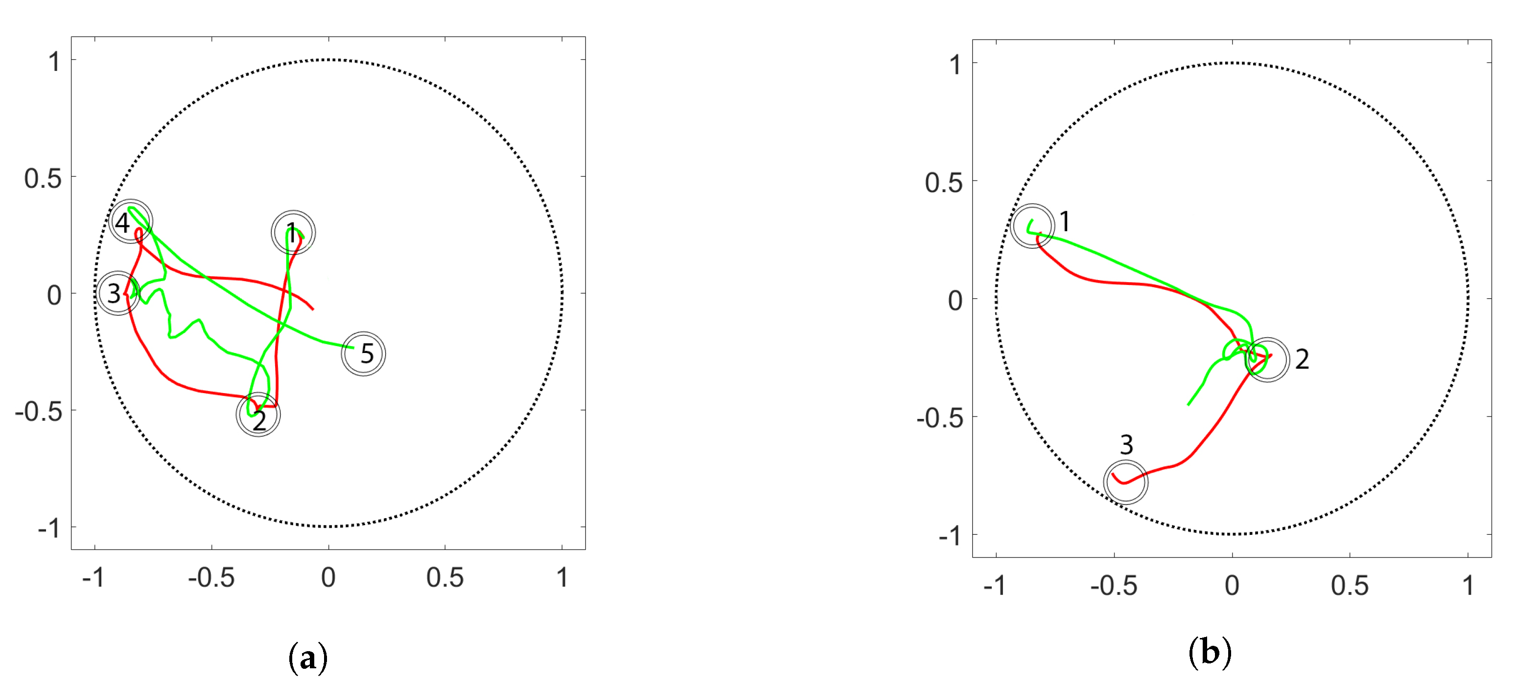
In order to show a visual interpretation of some trajectory patterns examples that determine the global PE values, Figure 7a shows the paths traveled by two users: participant #1 (red curve) and participant #5 (green curve) for targets 1 to 5. It is clear that the path between targets 2 and 3 was smoother for subject #1. The longer path traveled by subject #5 translated into a lower PE compared to subject #1 PE. There were other trajectory behaviors in this timespan that were related to the path efficiency. Note that the red trajectory was smoother not only between targets but also in the transition (when one target was achieved and the next one was shown to the user). On the contrary, the green line is slightly advanced than the red line; the user chose between a faster movement with the risk of a potential instability or at least more attention since muscle activity translates into more erratic trajectories and a smooth movement where inertia can be sometimes an annoying issue depending on the subject perception.
In Figure 7b, we show the trajectories for subjects #1 (red line) and #3 (green line) moving from target 1 to 2 and then to target 3 on test 5. The performance in this timespan gives us a visual example of the AR metric values. It is clear that subject #3 had difficulty maintaining the position in target 2. He achieved target 2 easily from target 1 but could not remain into the circle for two consecutive seconds. He left and entered the circle several times. As a consequence, the attempt ratio was increased indicating a less stable position control; also, the completion time metric was increased, i.e., it was delayed with respect the path defined by subject #1. As we can see in Figure 7, subject #1 was able to arrive to the third target while subject #3 was still in between. This effect seems to be repeated occasionally as we can see in Table 1 comparing the AR and CT values for both participants.
Analyzing statistical relationships between the different performance metrics, we found a positive correlation between the CR and PE and a negative correlation between the CR and AR. This is in accordance with the expected values. A high CR means that few targets were missed, so the subject was accomplishing the task; i.e., the path efficiency must be high and the attempt ratio must be low in those cases. We also obtained a negative correlation between the path efficiency and the attempt ratio. However, the time required to complete the experiments is independent of the other metrics.

3.2. Arm Position Experiment

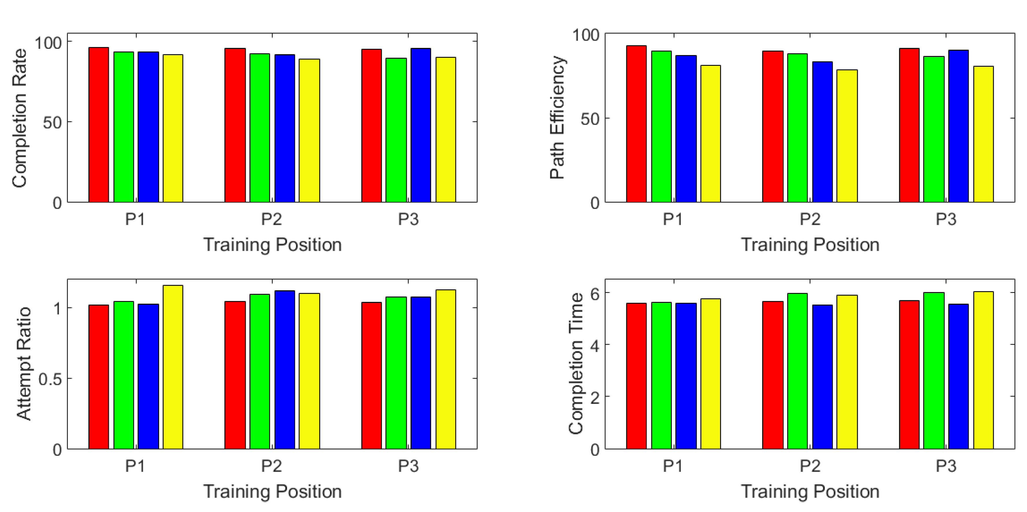
The arm position experiment was developed to test the robustness of a model in unknown arm positions (different to the trained one) and also to study if any of the training positions obtains better results. The mean values for each metric, training and testing position are shown in Figure 8. The free arm positioning was called P4 to simplify the notation.
The exact mean values are shown in Table 2, Table 3, Table 4 and Table 5.
Figure 8 plots the data for every test. Our results clearly show that the performance is high regardless the learning position or the training position. The minimum CR = 89.58 % is obtained for the model trained in P3 when tested in P2; the rest of the CR values are above 91%. The PE values are also high independently of the combination, with PE 83 % . The system was robust against arm positioning variations. Figure 8 also shows that the trend inside each training arm position is consistent with all the different training options, i.e., the bars follow a similar pattern for all the training arm positions. This confirms that the results were independent of the training position.
The results in Figure 8 indicate that P1 was the best testing position. Position P1 (red bars) performed slightly better than P2 (green bars) and P3 (blue bars) in almost all metrics, independently of the training arm position.
We applied the non parametric Friedman test for repeated measures to each training position. The results revealed a statistically significant difference for the PE metric with values of p = 0.0112 , 0.0129 , 0.0194 for the three different training positions. A posterior multiple comparison test indicated that the difference was between testing in P1 and testing in P4 (free movements) in all cases. After ranking the PE for the different training positions, P1 was always ranked in the first place and P4 in the last position in all experiments except one.
We also observed qualitative results related to the effect of fatigue and usability. All the patients reported ending up very tired after performing the test in P3. Holding the arm straight generated shoulder fatigue that did not allow the patients to keep a consistent performance. Some participants even stopped at some point to relax the arm. This observation is related to the quantitative results seen before, where P3 tests have lower PE values training in P1 an P2. This effect was mitigated when P3 was the training arm position because the fatigue was included in the training information.
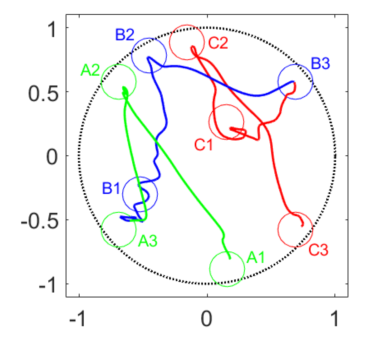
The yellow bars in Figure 8 give information about the system robustness against arm position changes within short periods of time (P4). These tests were performed allowing the users to move the arm with no restrictions at all, making every test unique and, therefore, not comparable with any other test. In any case, the results showed that all the metrics had an expected drop in this dynamic and uncertain scenario. The user adaptation was proven to be essential in this case. The participants managed to maintain a high performance (CR = 90.28% and PE = 80.13% on average). However, the system and the user needed a moment after changing the arm position to adapt to the EMG variations of it. Changing the arm position generated a transitory state in the EMG where the muscle activation was the result of changing the arm position and not due to the controller. Added to this effect, because of having a new arm position, the EMG patterns differ from one position to the other, so the user has to find again the correct activation patterns for the control. This process would take a small amount of time but enough to generate an unavoidable decay of the metrics. After this, the users performed consistently again until the next arm change.
An example of this is illustrated in Figure 9. In order to prove the robustness against the disturbance, we can analyze the behavior in these situations. Figure 9 demonstrates how the participant presents a high PE before changing the arm position (before reaching A3 and B3). After moving the arm to the new position, there was a drop in the PE (after leaving A3 and B3) followed by the user reaction against the drop, successfully recovering the high PE.

4. Discussion

An important handicap of the current myoelectric prostheses controls is the performance degradation suffered facing daily EMG pattern alterations. These effects emerge as a result of “noisy” factors that alter the input data. An ideal control should overcome these disturbances and last for a long time under different real-life scenarios before the performance starts to degrade and a re-calibration is necessary. In this manuscript, we have analyzed whether the adaptive IIR linear filtering control previously described [49] satisfies these robustness requirements for an optimal prostheses control. The results demonstrate that the performance of this recently proposed method was not affected by the time elapsed since training or the small electrode shifting deviations due to donning/doffing the armband in consecutive days that alter the EMG patterns. Moreover, we also show that the models trained in a specific arm position kept the high performance in other arm positions and that this position can be changed at any time. Thus, the important novelty of this work relies on the capabilities of the algorithm to stay stable through different disturbances without any re-adjustment. In spite of the encouraging results, a larger number of subjects must be tested in order to enhance the statistical confidence in the results reported in this paper. In addition, we have to experiment with limb deficiency subjects in order to analyze if the robustness is maintained in real patients.
It has to be noted that in this study we used wrist movements to control the active DoFs. This is not a restrictive choice. As far as there are enough independent patterns, any muscle activation could be used as input even if the EMG patterns do not perform a natural movement as it could happen in participants with limb deficiencies. For some patients, such as amputees, the limitation in the EMG signals that they can generate will limit the number of DoFs and the pattern selection. At the end, EMG patterns will be mapped to the available movements in the prosthesis no matter which is the biological origin. If desired, the EMG patterns could be selected to match the prosthesis functions. In summary, the algorithm performance relies only on the independence of the EMG signal patterns and not on the biological movement related to them. Of course, the larger the signal to noise ratio, the better the system will be able to map the EMG signals into the desired movements.
In order to exploit the benefits of the algorithm, the training protocol was implemented as a co-adaptive task in real-time. Due to the IIR adaptive algorithm characteristics (the previous estimated output is used to estimate the next output in addition to the new EMG signals), the system was able to learn the dynamics of the user-computer interaction in real time, avoiding any post processing and allowing to obtain a velocity controller in a natural way. If one of the agents does not operate properly, the other part will become confused, affecting its learning and performance. In practice, it means that the user must try to generate similar EMG patterns for a given movement. This is the main advantage of using an adaptive filtering approach: the learning of a continuous and dynamic environment enhances the capability to overcome small variances in the input data.
A first approach focused on the effect of small electrode shifting and the time that alters the EMG patterns. The donning/doffing experiment proved that the models learned in a short training (128 s) are usable for at least four days, keeping a high performance. Neither the removal of the sensor nor the long-term use affected the system behavior. In some ongoing tests, some patients have been using the same model for months without significant degradation. These observations strongly support that the model is robust enough to overcome these two real life disturbances. Previously, the FIR version of the model [51] was tested against similar disturbances in [39] being significantly affected by the donning/doffing of the electrodes. Overcoming these disturbances is another benefit of the novel IIR version.
Another important aspect of the study is the analysis of the influence of arm position. Modifying the arm posture introduces other disturbance sources as gravity, fatigue or EMG offsets that alter the initial EMG patterns. The results proved that the model was able to generalize from single arm positions to unknown situations keeping a high and stable performance. This is essential for a natural prosthesis control where the user has to be able to control the hand movement with similar EMG patterns no matter the position of the arm.
Other interesting observations came out from this experiment. Note that P1 position gave better results regardless of the training position used to learn the controller. Initially, one could expect that the best results during the test would be achieved by the same position used while training. One possible reason for these results is the effect that external conditions as fatigue or other muscle activity can generate in the system performance. In P1 position the arm is completely relaxed except for the active muscles used to perform the desired movement. Other positions (P2 and P3) require strength to hold the arm position, involving phenomena like gravity, fatigue or tension. These factors will generate and offset in the EMG patterns, non-related to the control task. The absence of this needless information and effort in P1 would be evidenced in a slight improvement on the performance metrics. Our findings also show that the algorithm is robust and efficient even in dynamic situations as the test P4, where participants reproduced a more realistic use. The change of the arm position every three targets generated a transient period where control became erratic since the signal to noise ratio became very low. However, this was quickly overcome by user adaptation, recovering the control and the high performance in a short time. On the other hand, none of the tested training positions seemed to be significantly better for training the model as we could have expected. This makes us think that the clue is again the consistency of the EMG patterns. As far as this is accomplished, this algorithm will learn a high performance model. This is possible thanks to the natural way in which the system learns that a velocity control is the best strategy. Note that in a system where the learning procedure is based on position control and during post-processing the velocity control is enforced, the system lacks the ability to respond in real time to changes in the input signal patterns. The observations proved that the model was robust enough against the EMG variations generated by different arm positions. This is strictly necessary for a natural prosthesis control where the users arm movements should not affect the prosthesis behavior.
In summary the new model has a high and robust performance in all the real life conditions presented for our able-bodied participants. After facing different types of disturbances that alter the EMG signals, we found out a general benefit of the new model applied to all of them. Since the robustness of the adaptive system is increased with respect to other controllers, it is also remarkable that the model does not need any adaptation or special training further than a basic and short initial training. This helps the user to understand and to increase the acceptance of this controller. The capability to overcome daily disturbances without re-calibrating or re-training the model is a great advantage for the user.
Our future work will replicate and extend in time these experiments in real patients to test if the system is also robust for end users with limb deficiencies in real life scenarios and to increase the number of participants. This future work is initially supported by the results shown in this paper for healthy subjects in real conditions and the fact that in [49] the behavior of the adaptive algorithm was similar for healthy and real patients in controlled conditions.

Author Contributions

Conceptualization, C.I. and J.I.; data curation, C.I.; dormal analysis, C.I. and J.I.; funding acquisition, C.I., A.C., E.J.B. and J.I.; investigation, C.I.; Methodology, C.I. and J.I.; project administration, C.I. and J.I.; resources, C.I.; software, C.I. and J.I.; supervision, J.I.; validation, C.I., A.C., E.J.B. and J.I.; visualization, C.I. and J.I.; writing—original draft, C.I. and J.I.; writing—review and editing, C.I., A.C., E.J.B. and J.I. All authors have read and agreed to the published version of the manuscript.

Funding

This research received no external funding.

Acknowledgments

This work is partially supported by Ministerio de Educacion, Cultura y Deporte (Spain) under grant FPU15/02870. The authors would like to thank Lucas Parra for the Myo device and Janne M. Hahne for discussions about the subject of the paper.

Conflicts of Interest

The authors declare no conflict of interest.

References

  1. Esquenazi, A. Amputation rehabilitation and prosthetic restoration. From surgery to community reintegration. Disabil. Rehabil. 2004, 26, 831–836. [Google Scholar] [CrossRef]
  2. Ziegler-Graham, K.; MacKenzie, E.J.; Ephraim, P.L.; Travison, T.G.; Brookmeyer, R. Estimating the Prevalence of Limb Loss in the United States: 2005 to 2050. Arch. Phys. Med. Rehabil. 2008, 89, 422–429. [Google Scholar] [CrossRef] [PubMed]
  3. Igual, C.; Pardo, L.A.; Hahne, J.M.; Igual, J.M. Myoelectric Control for Upper Limb Prostheses. Electronics 2019, 8, 1244. [Google Scholar] [CrossRef]
  4. Biddiss, E.; Chau, T. Upper-limb prosthetics: Critical factors in device abandonment. Am. J. Phys. Med. Rehabil. 2007, 86, 977–987. [Google Scholar] [CrossRef] [PubMed] [Green Version]
  5. Biddiss, E.A.; Chau, T.T. Upper limb prosthesis use and abandonment: A survey of the last 25 years. Prosthetics Orthot. Int. 2007, 31, 236–257. [Google Scholar] [CrossRef]
  6. Davidson, J. A survey of the satisfaction of upper limb amputees with their prostheses, their lifestyles, and their abilities. J. Hand Ther. 2002, 15, 62–70. [Google Scholar] [CrossRef]
  7. Datta, D.; Selvarajah, K.; Davey, N. Functional outcome of patients with proximal upper limb deficiency–acquired and congenital. Clin. Rehabil. 2004, 18, 172–177. [Google Scholar] [CrossRef]
  8. Vujaklija, I.; Farina, D.; Aszmann, O.C. New developments in prosthetic arm systems. Orthop. Res. Rev. 2016, 8, 31–39. [Google Scholar] [CrossRef] [Green Version]
  9. Scheme, E.J.; Englehart, K.B.; Hudgins, B.S. Selective classification for improved robustness of myoelectric control under nonideal conditions. IEEE Trans. Biomed. Eng. 2011, 58, 1698–1705. [Google Scholar] [CrossRef]
  10. Englehart, K.; Hudgins, B. A robust, real-time control scheme for multifunction myoelectric control. IEEE Trans. Biomed. Eng. 2003, 50, 848–854. [Google Scholar] [CrossRef]
  11. Parker, P.; Englehart, K.; Hudgins, B. Myoelectric signal processing for control of powered limb prostheses. J. Electromyogr. Kinesiol. 2006, 16, 541–548. [Google Scholar] [CrossRef] [PubMed]
  12. Fougner, A.; Stavdahl, Ø.; Kyberd, P.J.; Losier, Y.G.; Parker, P.A. Control of upper limb prostheses: Terminology and proportional myoelectric control—A review. IEEE Trans. Neural Syst. Rehabil. Eng. 2012, 20, 663–677. [Google Scholar] [CrossRef] [PubMed] [Green Version]
  13. Resnik, L.; Huang, H.H.; Winslow, A.; Crouch, D.L.; Zhang, F.; Wolk, N. Evaluation of EMG pattern recognition for upper limb prosthesis control: A case study in comparison with direct myoelectric control. J. Neuroeng. Rehabil. 2018, 15, 23. [Google Scholar] [CrossRef] [PubMed]
  14. Sartori, M.; Durandau, G.; Došen, S.; Farina, D. Robust simultaneous myoelectric control of multiple degrees of freedom in wrist-hand prostheses by real-time neuromusculoskeletal modeling. J. Neural Eng. 2018, 15, 066026. [Google Scholar] [CrossRef] [PubMed] [Green Version]
  15. Velliste, M.; Perel, S.; Spalding, M.C.; Whitford, A.S.; Schwartz, A.B. Cortical control of a prosthetic arm for self-feeding. Nature 2008, 453, 1098. [Google Scholar] [CrossRef] [PubMed]
  16. Amsuess, S.; Vujaklija, I.; Goebel, P.; Roche, A.D.; Graimann, B.; Aszmann, O.C.; Farina, D. Context-Dependent Upper Limb Prosthesis Control for Natural and Robust Use. IEEE Trans. Neural Syst. Rehabil. Eng. 2016, 24, 744–753. [Google Scholar] [CrossRef]
  17. Kuiken, T.A.; Miller, L.A.; Turner, K.; Hargrove, L.J. A comparison of pattern recognition control and direct control of a multiple degree-of-freedom transradial prosthesis. IEEE J. Transl. Eng. Health Med. 2016, 4, 1–8. [Google Scholar] [CrossRef]
  18. Phinyomark, A.N.; Khushaba, R.; Scheme, E. Feature Extraction and Selection for Myoelectric Control Based on Wearable EMG Sensors. Sensors 2018, 18, 1615. [Google Scholar] [CrossRef] [Green Version]
  19. Oskoei, M.A.; Hu, H. Myoelectric control systems—A survey. Biomed. Signal Process. Control 2007, 2, 275–294. [Google Scholar] [CrossRef]
  20. Spanias, J.A.; Perreault, E.J.; Hargrove, L.J. Detection of and compensation for EMG disturbances for powered lower limb prosthesis control. IEEE Trans. Neural Syst. Rehabil. Eng. 2015, 24, 226–234. [Google Scholar] [CrossRef]
  21. Rahimi, A.; Benatti, S.; Kanerva, P.; Benini, L.; Rabaey, J.M. Hyperdimensional biosignal processing: A case study for EMG-based hand gesture recognition. In Proceedings of the 2016 IEEE International Conference on Rebooting Computing (ICRC), Washington, DC, USA, 7–9 November 2016; pp. 1–8. [Google Scholar]
  22. Castellini, C.; van der Smagt, P. Surface EMG in advanced hand prosthetics. Biol. Cybern. 2009, 100, 35–47. [Google Scholar] [CrossRef] [PubMed] [Green Version]
  23. Ameri, A.; Akhaee, M.A.; Scheme, E.; Englehart, K. Regression convolutional neural network for improved simultaneous EMG control. J. Neural Eng. 2019, 16, 036015. [Google Scholar] [CrossRef] [PubMed]
  24. Hahne, J.; Biessmann, F.; Jiang, N.; Rehbaum, H.; Farina, D.; Meinecke, F.; Muller, K.R.; Parra, L. Linear and nonlinear regression techniques for simultaneous and proportional myoelectric control. IEEE Trans. Neural Syst. Rehabil. Eng. 2014, 22, 269–279. [Google Scholar] [CrossRef] [PubMed]
  25. Jiang, N.; Dosen, S.; Muller, K.; Farina, D. Myoelectric Control of Artificial Limbs—Is There a Need to Change Focus? IEEE Signal Process. Mag. 2012, 29. Available online: https://ieeexplore.ieee.org/document/6279589 (accessed on 20 February 2020).
  26. Ameri, A.; Scheme, E.; Kamavuako, E.; Englehart, K.; Parker, P. Real-Time, Simultaneous Myoelectric Control Using Force and Position-Based Training Paradigms. IEEE Trans. Biomed. Eng. 2014, 61, 279–287. [Google Scholar] [CrossRef]
  27. Hochberg, L.R.; Serruya, M.D.; Friehs, G.M.; Mukand, J.A.; Saleh, M.; Caplan, A.H.; Branner, A.; Chen, D.; Penn, R.D.; Donoghue, J.P. Neuronal ensemble control of prosthetic devices by a human with tetraplegia. Nature 2006, 442, 164. [Google Scholar] [CrossRef] [PubMed]
  28. Fang, Y.; Zhou, D.; Li, K.; Liu, H. Interface Prostheses With Classifier-Feedback-Based User Training. IEEE Trans. Biomed. Eng. 2017, 64, 2575–2583. [Google Scholar] [CrossRef] [Green Version]
  29. Thomas, N.; Ung, G.; McGarvey, C.; Brown, J.D. Comparison of vibrotactile and joint-torque feedback in a myoelectric upper-limb prosthesis. J. Neuroeng. Rehabil. 2019, 16, 70. [Google Scholar] [CrossRef] [Green Version]
  30. Guémann, M.; Bouvier, S.; Halgand, C.; Borrini, L.; Paclet, F.; Lapeyre, E.; Ricard, D.; Cattaert, D.; de Rugy, A. Sensory and motor parameter estimation for elbow myoelectric control with vibrotactile feedback. Ann. Phys. Rehabil. Med. 2018, 61, e467. [Google Scholar] [CrossRef]
  31. Markovic, M.; Schweisfurth, M.A.; Engels, L.F.; Farina, D.; Dosen, S. Myocontrol is closed-loop control: Incidental feedback is sufficient for scaling the prosthesis force in routine grasping. J. Neuroeng. Rehabil. 2018, 15, 81. [Google Scholar] [CrossRef]
  32. Pasquina, P.F.; Perry, B.N.; Miller, M.E.; Ling, G.S.; Tsao, J.W. Recent advances in bioelectric prostheses. Neurol. Clin. Pract. 2015, 5, 164–170. [Google Scholar] [CrossRef] [PubMed] [Green Version]
  33. Jiang, N.; Farina, D. Myoelectric control of upper limb prosthesis: Current status, challenges and recent advances. Front. Neuroeng. 2014, 4. [Google Scholar] [CrossRef]
  34. Lendaro, E.; Mastinu, E.; Håkansson, B.; Ortiz-Catalan, M. Real-time Classification of Non-Weight Bearing Lower-Limb Movements Using EMG to Facilitate Phantom Motor Execution: Engineering and Case Study Application on Phantom Limb Pain. Front. Neurol. 2017, 8, 470. [Google Scholar] [CrossRef] [PubMed] [Green Version]
  35. Mastinu, E.; Ortiz-Catalan, M.; Håkansson, B. Analog front-ends comparison in the way of a portable, low-power and low-cost EMG controller based on pattern recognition. In Proceedings of the 2015 37th Annual International Conference of the IEEE Engineering in Medicine and Biology Society (EMBC), Milan, Italy, 25–29 August 2015; pp. 2111–2114. [Google Scholar] [CrossRef] [Green Version]
  36. Beck, T.W.; Housh, T.J.; Cramer, J.T.; Malek, M.H.; Mielke, M.; Hendrix, R.; Weir, J.P. Electrode shift and normalization reduce the innervation zone’s influence on EMG. Med. Sci. Sport. Exerc. 2008, 40, 1314–1322. [Google Scholar] [CrossRef] [PubMed]
  37. Pasquina, P.F.; Evangelista, M.; Carvalho, A.; Lockhart, J.; Griffin, S.; Nanos, G.; McKay, P.; Hansen, M.; Ipsen, D.; Vandersea, J.; et al. First-in-man demonstration of a fully implanted myoelectric sensors system to control an advanced electromechanical prosthetic hand. J. Neurosci. Methods 2015, 244, 85–93. [Google Scholar] [CrossRef] [PubMed] [Green Version]
  38. Fougner, A.; Scheme, E.; Chan, A.D.C.; Englehart, K.; Stavdahl, O. Resolving the Limb Position Effect in Myoelectric Pattern Recognition. IEEE Trans. Neural Syst. Rehabil. Eng. 2011, 19, 644–651. [Google Scholar] [CrossRef] [PubMed] [Green Version]
  39. Hwang, H.J.; Hahne, J.; Mueller, K.R. Real-time robustness evaluation of regression based myoelectric control against arm position change and donning/doffing. PLoS ONE 2017, 12, e0186318. [Google Scholar] [CrossRef] [Green Version]
  40. Young, A.J.; Hargrove, L.J.; Kuiken, T.A. The effects of electrode size and orientation on the sensitivity of myoelectric pattern recognition systems to electrode shift. IEEE Trans. Biomed. Eng. 2011, 58, 2537–2544. [Google Scholar] [CrossRef] [Green Version]
  41. Prahm, C.; Schulz, A.; Paaßen, B.; Schoisswohl, J.; Kaniusas, E.; Dorffner, G.; Hammer, B.; Aszmann, O. Counteracting Electrode Shifts in Upper-Limb Prosthesis Control via Transfer Learning. IEEE Trans. Neural Syst. Rehabil. Eng. 2019, 27, 956–962. [Google Scholar] [CrossRef] [Green Version]
  42. Cipriani, C.; Sassu, R.; Controzzi, M.; Carrozza, M.C. Influence of the weight actions of the hand prosthesis on the performance of pattern recognition based myoelectric control: Preliminary study. In Proceedings of the 2011 Annual International Conference of the IEEE Engineering in Medicine and Biology Society, Boston, MA, USA, 30 August–3 September 2011; pp. 1620–1623. [Google Scholar] [CrossRef]
  43. Amsuess, S.; Paredes, L.P.; Rudigkeit, N.; Graimann, B.; Herrmann, M.J.; Farina, D. Long term stability of surface EMG pattern classification for prosthetic control. In Proceedings of the 2013 35th Annual International Conference of the IEEE Engineering in Medicine and Biology Society (EMBC), Osaka, Japan, 3–7 July 2013; pp. 3622–3625. [Google Scholar] [CrossRef]
  44. Scheme, E.; Englehart, K. Electromyogram pattern recognition for control of powered upper-limb prostheses: State of the art and challenges for clinical use. J. Rehabil. Res. Dev. 2011, 48, 643–659. [Google Scholar] [CrossRef]
  45. Scheme, E.; Fougner, A.; Stavdahl, O.; Chan, A.D.C.; Englehart, K. Examining the adverse effects of limb position on pattern recognition based myoelectric control. In Proceedings of the 2010 Annual International Conference of the IEEE Engineering in Medicine and Biology, Buenos Aires, Argentina, 31 August–4 September 2010; pp. 6337–6340. [Google Scholar] [CrossRef] [Green Version]
  46. Dohnálek, P.; Gajdoš, P.; Peterek, T. Human activity recognition on raw sensor data via sparse approximation. In Proceedings of the 2013 36th International Conference on Telecommunications and Signal Processing (TSP), Rome, Italy, 2–4 July 2013; pp. 700–703. [Google Scholar] [CrossRef]
  47. Marasco, P.D.; Hebert, J.S.; Sensinger, J.W.; Shell, C.E.; Schofield, J.S.; Thumser, Z.C.; Nataraj, R.; Beckler, D.T.; Dawson, M.R.; Blustein, D.H.; et al. Illusory movement perception improves motor control for prosthetic hands. Sci. Transl. Med. 2018, 10. [Google Scholar] [CrossRef] [PubMed] [Green Version]
  48. Mastinu, E.; Doguet, P.; Botquin, Y.; Håkansson, B.; Ortiz-Catalan, M. Embedded System for Prosthetic Control Using Implanted Neuromuscular Interfaces Accessed Via an Osseointegrated Implant. IEEE Trans. Biomed. Circuits Syst. 2017, 11, 867–877. [Google Scholar] [CrossRef] [PubMed]
  49. Igual, C.; Igual, J.; Hahne, J.M.; Parra, L.C. Adaptive Auto-Regressive Proportional Myoelectric Control. IEEE Trans. Neural Syst. Rehabil. Eng. 2019, 27, 314–322. [Google Scholar] [CrossRef] [PubMed]
  50. Huang, Y.; Englehart, K.B.; Hudgins, B.; Chan, A.D. A Gaussian mixture model based classification scheme for myoelectric control of powered upper limb prostheses. IEEE Trans. Biomed. Eng. 2005, 52, 1801–1811. [Google Scholar] [CrossRef]
  51. Hahne, J.M.; Dähne, S.; Hwang, H.J.; Müller, K.R.; Parra, L.C. Concurrent adaptation of human and machine improves simultaneous and proportional myoelectric control. IEEE Trans. Neural Syst. Rehabil. Eng. 2015, 23, 618–627. [Google Scholar] [CrossRef]
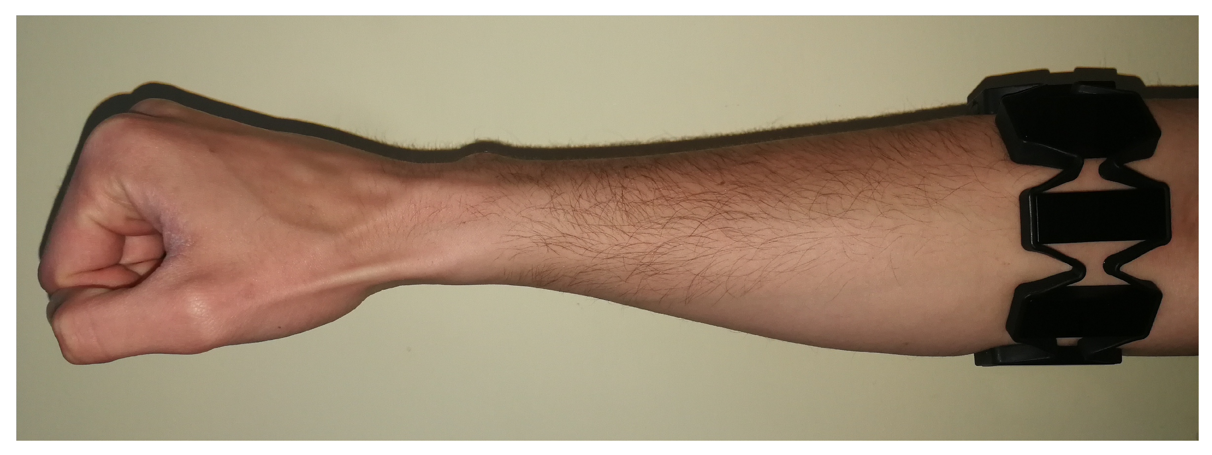
Figure 1. Myo Armband positioning in the forearm of an able bodied participant.
Applsci 10 02892 g001
Figure 2. (a) Training UI. The user position is displayed as a red cross. The target is the big green circle that moves around the space. The anticipated movement of the target is represented by the three small green circles. The orange arrow shows the direction of the error. (b) Test UI. Similar to the training UI with small changes. The targets are switched to orange to differentiate the test phase from the training phase. The trace circles are no more displayed as the targets are now static. The error direction is not shown since we are testing not training.
Applsci 10 02892 g002
Figure 3. Donning/Doffing experimental protocol scheme. All test sessions used the same model learned on day 1 training session. Five tests were performed after the training session. First, a baseline test is executed immediately after completing the training, so the differences between testing and training conditions are minimal. Afterwards, starting at the same day, one test per day is performed. The donning and doffing of the Myo Armband was carried out on the first day between the baseline test 1 and test 2 and between experimental days.
Applsci 10 02892 g003
Figure 4. The three arm positions used as training arm positions. Each position involves different muscle activation and has different effects from gravity and fatigue. P1: Arm fully extended pointing down with the wrist. P2: Arm pointing front with the wrist and elbow flexed 90 degrees. P3: Arm fully extended pointing front.
Applsci 10 02892 g004
Figure 5. Box and whisker plot for the Completion Rate (CR), Path Efficiency (PE), Attempt Ratio (AR) and Completion Time (CT) for each participant. Except for patient 6’s PE value, the rest of the boxes show a small variance. This is proof of a consistent behavior through time.
Applsci 10 02892 g005
Figure 6. PE for subject #6 (blue line) and average PE value between all participants (black line) vs. the day of experiment. This figure explains that the larger variance of the PE value for that participant is not due to instability problems of the algorithm but to his learning process (his performance improved significantly from test 1 to 5). Once the learning saturates (as we can see in the last two tests), the behavior started to be more stable like the other participants results.
Applsci 10 02892 g006
Figure 7. (a) Path for test 5 for subjects 1 (red) and 5 (green) for the first five targets. This is a comparison between a high PE and a lower PE value. Green path shows a more erratic behavior reaching a lower PE value as the red path follows an almost straight trajectory from target to target with a high PE value. (b) This is an attempt ratio value example showing the stability of the controller to maintain a position. Red line corresponds to subject 1; green line corresponds to subject 3. The subject 1 entered the target 2 and remained inside at the first try. Opposed to this, subject 3 entered and left the target two times until the target was missed. The participant, in this occasion, was not able to maintain the position having a less stable control measured by the attempt ratio value.
Applsci 10 02892 g007
Figure 8. Mean CR (top-left), PE (top-right), AR (bottom-left) and CT (bottom-right). The horizontal axes are the training positions. The color bars represent the arm position during the test: P1 for the red bars, P2 for the green bars, P3 for the blue bars and yellow when there were no restrictions in the arm position P4. The height of the bar indicates the corresponding metric average value between all participants.
Applsci 10 02892 g008
Figure 9. Trajectories during free arm position test. During this test, the participants were asked to change the arm position every three targets. Each color represents the estimations for the period of time (three targets) that one arm position was held. Three sets of three targets and the trajectories that followed between them are plotted: Set A (green), Set B (blue) and Set C (red). Starting from A1, after reaching the last target of each set, A3 and B3 (which means changing the arm position), the plot shows how the trajectories became more erratic. Once the user adapted to the new position, the behavior returned to a smooth control.
Applsci 10 02892 g009
Table 1. Performance metrics for the eight participants in the donning/doffing experiment. The metrics tabled are completion rate as the completed targets over the total targets, path efficiency as the shortest distance over the total distance traveled, the completion time as seconds per target and the attempt ratio as number of attempts to hit a target. Each row presents the results for one participant showing the value and the variance for each metric. Last row is the average of all subjects.
ParticipantCompletion Rate (%)Path Efficiency (%)Completion Time (s)Attempt Ratio
199.44 ± 1.2490.75 ± 1.865.338 ± 0.3871.017 ± 0.025
297.78 ± 3.6287.20 ± 1.955.554 ± 0.2301.046 ± 0.034
395.00 ± 2.3275.32 ± 4.006.153 ± 0.3211.212 ± 0.076
498.33 ± 2.4992.28 ± 2.406.151 ± 0.2301.049 ± 0.066
592.22 ± 3.6273.42 ± 3.075.673 ± 0.3881.151 ± 0.087
695.55 ± 4.6582.56 ± 7.855.740 ± 0.4991.121 ± 0.116
795.00 ± 3.6279.90 ± 4.035.568 ± 0.2571.070 ± 0.060
893.33 ± 2.4892.14 ± 1.985.994 ± 0.2171.053 ± 0.047
Avg95.83 ± 3.0084.19 ± 3.395.771 ± 0.3161.090 ± 0.064
Table 2. Average Completion Rate metric among all users for different training and test arm positions. Each row indicates the arm position used to train the model. Each column indicates the arm position used to test the model.
TrainingTest P1Test P2Test P3Test P4
P196.5393.7593.7591.67
P295.8392.3691.6788.89
P395.1489.5895.8490.28
Table 3. Average Path Efficiency metric among all users for different training and test arm positions. Each row indicates the arm position used to train the model. Each column indicates the arm position used to test the model.
TrainingTest P1Test P2Test P3Test P4
P192.9189.8586.8781.32
P289.7888.0683.5078.22
P391.3086.3490.3180.84
Table 4. Average Attempt Ratio metric among all users for different training and test arm positions. Each row indicates the arm position used to train the model. Each column indicates the arm position used to test the model.
TrainingTest P1Test P2Test P3Test P4
P11.0221.0451.0221.159
P21.0451.0941.1181.104
P31.0381.0741.0761.128
Table 5. Average Completion Time metric among all users for different training and test arm positions. Each row indicates the arm position used to train the model. Each column indicates the arm position used to test the model.
TrainingTest P1Test P2Test P3Test P4
P15.5735.6325.5905.776
P25.6435.9505.5365.908
P35.6906.0015.5496.037