Article

An Unsupervised Regularization and Dropout based Deep Neural Network and Its Application for Thermal Error Prediction

1
School of Mechanical Engineering, Shenyang Ligong University, Shenyang 110159, China
2
Civil & Environmental Engineering at University of Waterloo, Waterloo, ON N2L3G1, Canada
3
Cambridge Data Technology (Shenzhen) LTD, Shenzhen 518042, China
*
Author to whom correspondence should be addressed.
Appl. Sci. 2020, 10(8), 2870; https://doi.org/10.3390/app10082870
Submission received: 25 February 2020 / Revised: 30 March 2020 / Accepted: 13 April 2020 / Published: 21 April 2020

Abstract

:
Due to the large size of the heavy duty machine tool-foundation systems, space temperature difference is high related to thermal error, which affects to system’s accuracy greatly. The recent highly focused deep learning technology could be an alternative in thermal error prediction. In this paper, a thermal prediction model based on a self-organizing deep neural network (DNN) is developed to facilitate accurate-based training for thermal error modeling of heavy-duty machine tool-foundation systems. The proposed model is improved in two ways. Firstly, a dropout self-organizing mechanism for unsupervised training is developed to prevent co-adaptation of the feature detectors. In addition, a regularization enhanced transfer function is proposed to further reduce the less important weights of the process and improve the network feature extraction capability and generalization ability. Furthermore, temperature sensors are used to acquire temperature data from the heavy-duty machine tool and concrete foundation. In this way, sample data of thermal error predictive model are repeatedly collected from the same locations at different times. Finally, accuracy of the thermal error prediction model was validated by thermal error experiments, thus laying the foundation for subsequent studies on thermal error compensation.

1. Introduction

Environmental temperature has an enormous influence on large machine tools with regards to thermal error, which is different from the effect on ordinary-sized machine tools [1]. Thermal gradients cause heat to flow through the machine structure and result in non-linear structural error whether the machine is in operation or in a static mode [2]. It has been verified that thermally induced error accounts for 40%–70% of total errors [3,4], and its effect on machine tools has become a well-recognized engineering problem in response to the increasing requirement of product quality [5]. As a result, reduction of thermal error is quite beneficial for a high-precision manufacturing system [6]. Besides, the coordinate offset is modified in the numerical control program according to the error value, so that the thermal error of the machine tool can be reduced.
In the working cycle of a machine tool, the thermal errors are time-variant according to the change of environment and operating conditions. As far as most modeling methods are concerned, the thermal error models are all obtained by finding the best mapping relations between the thermal errors and some key temperature variables related to the heat source location [7]. Li F [8] presented a novel approach in which a clustering method of temperature sensors was proposed, and the thermal error model of heavy machine tools was established. Chen made a multiple regression analysis and proposed the artificial neural network model for the real-time forecast of thermal errors with numerous temperature measurements [9]. Lee et al. presented a thermal modeling method based on independent component analysis to compensate for the thermal errors of a commercial machining center [10]. Jianguo Yang et al. [11,12] proposed several methods to optimize the selection of minimum number of thermal sensors for machine tool thermal error compensation, such as ant colony algorithm-based back propagation neural network and synthetic grey correlation based grey neural network. Wang L et al. [13] proposed a hybrid thermal error modeling method to forecast the thermal expansion of a heavy boring and milling machine tool in z-axis.
The thermal error prediction model mainly depends on the accuracy and robustness of the input temperature variables and the error of the machine tool system. Gomez-Acedo, et al. [14], utilized the inductive sensors array to measure the thermal error of a large gantry-type machine tool. Lee, et al. found a more reliable and practical measuring principal and method to monitor the deformation of heavy-duty Computer Numerical Control (CNC) machine tool structures using laser interferometer [15]. In addition, a novel temperature sensor, fiber Bragg grating (FBG) sensor, was used to collect the surface temperature of the machine [16]. Gomez-Acedo E designed a set of laser interferometer single-point tracking measuring method for thermal deformation of heavy machine tools [17].
In summary, thermal error predictive models for heavy-duty machine tools have been previously established and reported in the literature. However, two additional factors should be taken into account: (1) due to variation in the ambient environment and working conditions, thermal error of the concrete foundation should not be neglected [18,19]; (2) in order to build accurate thermal error prediction model, it is necessary to build a neural network model with strong network feature extraction ability, generalization ability and network stability. To address these challenges, this paper proposes a self-organizing deep neural network (DNN) to improve the feature extraction capability and generalization ability of unsupervised training and to solve the problems of overfitting and lengthy training times. Deep neural network is one of the most commonly used tools in regression and prediction, and we propose that it could be a potential alternative to solve the particular problem in our domain. In this paper, an improved unsupervised training algorithm is proposed to significantly reduce the effects of less important weights in the neural network and to ensure the trained self-organizing DNN can more reasonably express the inherent features of the input data. Based on the above model, the thermal error of the heavy-duty machine tool -foundation systems are predicted accurately.

2. Self-Organizing Deep Neural Network

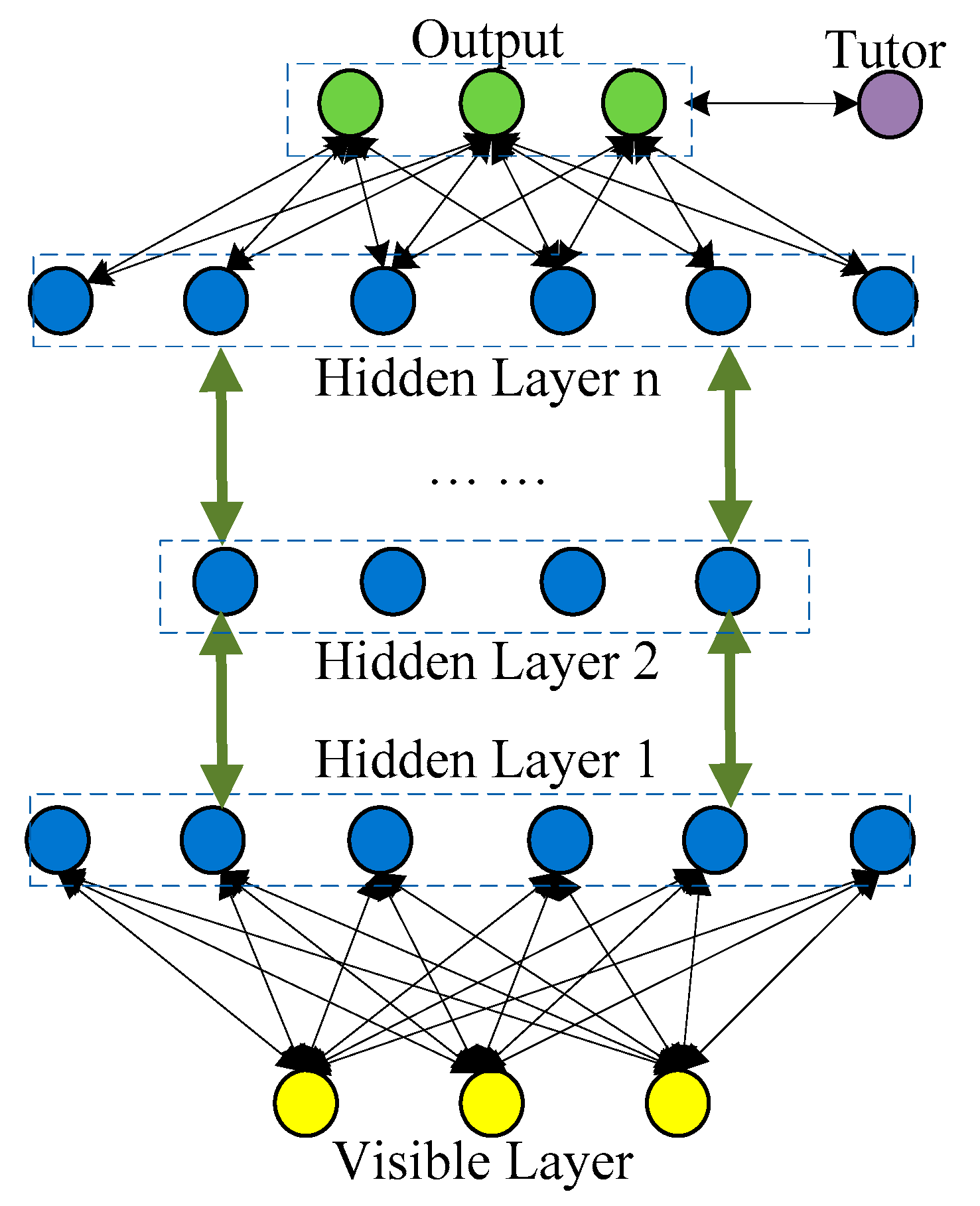
2.1. Network Structure

This paper proposes a self-organizing DNN structure, as shown in Figure 1. The network consists of four parts: input layer, hidden layer, output layer, and instructor signal layer. The first layer is the input layer (visible Layer, V) for receiving the original signal. The “training of a model” consists three steps, (1) build an artificial intelligence (AI) model; (2) prepare data to be trained, including model’s input and output; (3) use intelligent algorithm to teach the model to output data based on input data. The received signal is then passed to the hidden layer for feature extraction. The hidden layer is usually composed of 2–4 layers of neurons (hidden layer 1–4, L1–L4) depending on the size of the data. The number of neurons in each layer varies. During unsupervised training, V and L1 constitute the first restricted Boltzmann machine (RBM), L1 and L2 constitute the second RBM, and so on. Each RBM consists of a visual layer (input layer) and hidden layer (output layer), and the layers are connected via bi-directional connections (indicated by arrows in Figure 1). There are no connections within the same layer. During the process of unsupervised training, the hidden layer of each RBM is passed the data from the preceding RBM hidden layer and extracts one or more better and more abstract feature expressions from it. Then the feature data is passed to the output layer, which is the third part of the self-organizing DNN. The number of neurons in this layer is usually determined by the task. For example, in classification tasks, the number of neurons is the number of classifications. The function of the instructor signal layer is to provide the target signal for subsequent supervised learning.
A conventional DNN is obtained by superimposing several RBMs, and the training process is divided into the unsupervised and supervised parts. Layer-wise pre-training is also used in the unsupervised training process. The RBM training formulae are expressed as:
p ( h j = 1 ) = 1 1 + e b j i v i w i j
p ( v i = 1 ) = 1 1 + e c i j h j w j i
where v i is the value of the i th neuron in the visible layer, h j is the value of the j th neuron in the hidden layer, b and c are biases of the visible layer and hidden layer, respectively, and w i j represents the weight between the visible neuron i and hidden neuron j . Equations (1) and (2) are called the RBM knowledge learning (feature extraction) equation and knowledge inference (data reconstruction) equation, respectively. Let θ = ( W , b , c ) . Then, in accordance with the contrastive divergence algorithm, the weight and bias update formulae for unsupervised training are:
Δ θ = h j 0 v i 0 h j 1 v i 1
θ n = Δ θ + θ 0
where · represents the average of the dot product of posterior distribution, h j 0 v i 0 and θ 0 represent the initial state and initial parameters, respectively, h j 1 v i 1 is the product of the visual layer and hidden layer after a Markov chain operation, Δ θ represents the parameter change, and θ n is the obtained weight and offset.
The self-organizing DNN training process proposed in this paper is divided into two steps. First, each RBM is trained using the greedy layer-wise unsupervised training method, during which adaptive dropout is used to automatically adjust the network structure, thereby decoupling the feature detectors. A regularization enhancement transfer function is designed to introduce the regularization enhancement terms. This term speeds up the process of reducing the number of neural network weights and thereby improves the neural network feature extraction and data reconstruction capabilities. At the same time, contrastive divergence (CD, which means apply weights update only once after epoch training) algorithm is used for weight adjustment [20]. The output of each RBM is used as the input to the next RBM, and the training process continues in this way until the last layer. Second, the network is expanded into a forward neural network, in which all neurons are fixed in their respective positions. Then the backpropagation (BP) neural network algorithm is used to conduct local optimization and to fine-tune the network weights.

2.2. Self-Organization Algorithm for Unsupervised Training

During the conventional DNN training process, if the network size is relatively large in relation to the training data, the trained network often performs poorly during testing. This is due to the over-training or overfitting phenomena of the network based on patterns of the training dataset. Since the network treats each sample of the training set as independent and ignores the correlation between samples as part of the whole, error information and error features are learned along with other useful information. Therefore, although good results seem to be achieved after the neural network has been trained with a training dataset, the trained network is often insensitive to unknown test data. In a DNN, neurons (feature detectors) in the same hidden layer should be independent of each other (activated and sparsely distributed) due to the absence of lateral inhibition weight connections. However, due to the explaining away phenomenon, synergy often occurs between neurons, meaning one neuron can easily influence another in the same layer. When a feature detector learns the wrong features, these incorrect features are likely to filter through to other feature detectors, resulting in overfitting and poor test results. Hinton et al. proposed a dropout self-organization strategy and obtained satisfactory results. In their model, applying the dropout strategy in supervised training prevented synergy between neurons during training. Improvements were achieved to varying degrees in a number of benchmark tests and new records were set in certain pattern recognition tasks [21,22].
In this paper, dropout and regularization enhancement terms are introduced into the unsupervised training. Each neuron in the hidden layer is randomly removed with a certain probability (only neurons are removed, and connection weights are retained). The removed neurons will not be part of the neural network for the time being, thus their state values and connection weights are not updated. After the neural network performs a weight update operation, the removed neurons are returned to their original positions, and another batch of neurons are removed with the same probability and the same operation is performed again. In this process, an upper limit of the L2 norm is preset for the weight of each neuron in the hidden layer. If the weight exceeds the upper limit after being updated, the weight is normalized. This ensures a better solution space for weights in the global scope with a better learning rate. In the test phase, the mean network method is used to calculate the output of the forward network. That is, all neurons are activated, and their weights are reduced at a certain rate so that they can be used in the test set. The dropout formulae designed for the unsupervised process is expressed as:
h j = h j 0 · d r F
d r F = { 1 ,   P f r d r 0 ,   P f < r d r
where h j 0 is the state value of the j th unit of the hidden layer calculated by Equation (1), and h j is the new value of hidden neuron j , d r F determines whether the unit should be removed in a certain operation, P f represents the random decision probability, and r d r is the preset probability threshold (determines the percentage of hidden layer neurons to be removed each time). According to Equations (5) and (6), when P f r d r , the j th neuron is retained and its weight is updated. If P f < r d r , the j th neuron is removed in this operation. In each CD operation, dropout is designed to calculate the intermediate state h j 0 in the v i 1 process. Note that in some special tasks, such as time sequence prediction, visual layer neurons cannot be removed because they contain temporal logic information, therefore dropout is only used in the v i 1 operation.
Figure 2 illustrates the dropout process in unsupervised learning. During this process, in accordance with Equations (5) and (6), values of neurons in the hidden layer that are selected at random are set to zero. For a neuron with a dashed line, h m indicates that it has been randomly chosen and temporarily removed. When the iteration (epoch) is over, the neuron will be activated and return to the hidden layer to participate in the next iteration. Through automatic adjustment of the neural network structure, this strategy ensures that two neurons in the same layer do not always appear in the same iteration, forcing them to learn more feature knowledge and seek better solutions. To some extent, this prevents the occurrence of synergy between some of the feature detectors. Dropout can be regarded as a work mode similar to the mean network. Since neurons are randomly removed in each cycle, the network structure changes after each iteration. However, all neurons will be activated and participate in the testing process during the final test phase.
Training a neural network with a limited number of samples often results in more than one model (network structure). In other words, there are many, even countless, models that can fit the target values, although some models are very close to actual expectations. To choose a better model, the training goal often needs to be regularized. This regularization ensures the network structure not only meets the training error requirements, but also meets other requirements such as scale and weight. A balance must be struck between these two goals in the training result. An additional aim of Bayesian regularization is to make sure the neural network meets the following requirements: (1) the training error must be small enough; (2) the magnitude of the network weight scale is as small as possible. Dropout can also be regarded as generalized Bayesian regularization. In generalized Bayesian regularization, it must be assumed that the feature detectors are independent of each other. The dropout mechanism forces the neurons to be independent, and therefore effectively prevents overfitting. Since the dropout rate in Equation (6), i.e., r d r , still needs to be determined by practical measurement, the mutual independence of the feature detectors can only be increased to a certain extent, and the randomness leads to additional instability. In order to more effectively prevent overfitting and improve the efficiency of unsupervised training, the dropout mechanism can be employed, and a regularization enhancement method is designed for the transfer function.
In the self-organizing DNN, the values of neurons in the hidden layer are discrete numbers, either 0 or 1, which means the traditional regularization method cannot be applied directly. Here, the introduction of a regularization enhancement factor is proposed and a new transfer function is constructed as follows:
F W = α P + β E W
P = P ( v , h ) e x p ( E ( v , h ) ) = e h T W v + b T v + c T h
E W = 1 m × n j = 1 m i = 1 n w i j 2
where F W is the new objective function in unsupervised training, P is the original objective function (the joint probability distribution of the visible layer and hidden layer of the network), E W is the regularization enhancement factor, expressed in the same form as Equation (9), w i j represents the weights of neuron i and hidden layer neuron j , m and n are the total numbers of neurons in the two layers, respectively, and α and β are performance parameters that must be specified at the beginning of training.
If   α     β , then P is the dominant factor of F W in Equation (7) and the main goal of training. As the network training progresses, the number of energy functions is reduced, that is, the joint probability distribution increases. In particular, if α = 1 ,   β = 0 , then there is F W = P , if so, Equation (7) is equal to Equation (8) because the coefficient of β is 0. On the other hand, if α     β , E W becomes the main training goal during training, the network weights decrease with each iteration. Therefore, by introducing a regularization enhancement factor that acts on the weights of neurons that have survived the dropout process, the number of less important weights that have less influence on the output are reduced. This ensures that only some of the neurons learn important information, i.e., features, and prevents overfitting during training. Moreover, the use of the regularization reinforcement term improves the convergence of the neural network weights in the improved solution space, and is faster and more stable.
The neural network toolbox can be used with the traditional method of obtaining α and β . In this process, the weight is treated as a random variable and it is assumed that the prior probabilities, P and E W , are Gaussian functions. The two performance parameters can be obtained using the Bayesian criterion. However, in DNN, the hidden layer neurons are discrete binary values, therefore conventional methods cannot be used to calculate the Hessian matrix. In this paper, performance parameters α and β are preset values. Now, the transfer function of unsupervised learning can be expressed as:
F w = l o g P ( v , h ) θ + 2 m × n j = 1 m i = 1 n w i j
As a result, when training a self-organizing DBN, Fomulas (1), (2) and (10) are applied, where dropout and regularization enhanced factors are superposed, and the weights are still updated by contrastive divergence (CD) algorithm, as shown in the following formula:
Δ w i j = η w ( v i 0 h j 0 v i 1 h j 1 )
Δ b = η b b 2 ( h j 0 2 h j 1 2 )
Δ c = η c c 2 ( v i 0 2 v i 1 2 )
where, η w , η b and η c are the updated rates of the weight and bias values, the definition of · is the same as Equation (3). During the n th iteration, the updated weight and biases are:
w i j ( n ) = w i j ( n 1 ) + Δ w i j ( n )
b ( n ) = b ( n 1 ) + Δ b ( n )
c ( n ) = c ( n 1 ) + Δ c ( n )
where n is the n th epoch.

2.3. Supervised Training Algorithm

The backpropagation (BP) algorithm is used in supervised training of the self-organizing DNN. The last layer of the neural network receives the output of the last RBM. The difference between the actual signal and the network output signal produces a feedback error. The error is used to perform local adjustments of the overall weights of the neural network. The process is divided into two steps: First, the self-organizing DNN is expanded into a forward network and the data signal is transmitted to the input layer, then to the next layer, and so on until the output layer; second, the backpropagation error is generated for fine tuning the neural network parameters. The specific steps are as follows:
(1)
Initialize the forward neural network, set the step length to K .
(2)
Calculate the forward output,
y j ( l ) =   w i j y j ( l 1 )
where y j ( l ) is the output of the j th neuron of the l th layer.
(3)
Calculate the error signal based on:
e j = R j Y j
where R represents the teacher’s signal, which represents ideal predicted temperature, and it is taken by hand when the whole dataset is processed in experiment. Y is the value of output layer, and e the error signal.
(4)
Generate the backpropagation error. For neurons in the output layer, this is:
δ j ( l ) = e j Y j [ 1 Y j ]
For neurons in the hidden layer, we have:
δ j ( l 1 ) = y j ( l ) [ 1 y j ( l ) ] ·   δ j ( l ) w i j ( l )
(5)
Modify the weights based on:
w i j ( l ) = w i j ( l ) + η δ j y j ( l )
where η is the learning rate.
(6)
When the iteration reaches K , terminate the loop; otherwise, return to Step (2).
During unsupervised training, the regularization enhancement factor does not change the calculation processes of the visible layer and hidden layer, as shown in Equation (7). Instead, the weights of the network are adjusted only by affecting the shares of the two parts of the new objective function. Moreover, the value range of the neural network unit does not change (0 and 1). The combined effect of the above factors is that unsupervised process of self-organizing DNN must also converge under the same condition as the conventional unsupervised process. The conventional BP algorithm is used during supervised training. In accordance with the Weierstrass approximation theorem [23], the supervised process must converge.
In this section, the detailed training processes (including unsupervised and supervised training) and the improvements (unsupervised-dropout and unsupervised-regularization) have been fully introduced. In next section, the improved model will be proposed as an alternative to thermal error modeling, because (1) DNN, proposed as a big data technology, has been proved great successes on many feature learning problems; (2) the process of unsupervised learning has been improved in two ways, which have greatly increased DNN’s feature learning and regression ability; (3) to solve thermal error modeling, a big data method is required because feature learning is very important in this process, besides, thermal error data is used as input and temperature data is used as output, which is a classic regression problem.

3. Experimental Validation

3.1. Experimental Setup

The steps of self-organizing DNN unsupervised training are as follows:
(1)
Set the network size according to the training data (including the number of hidden layers and the number of neurons in each layer) and initialize the network parameters.
(2)
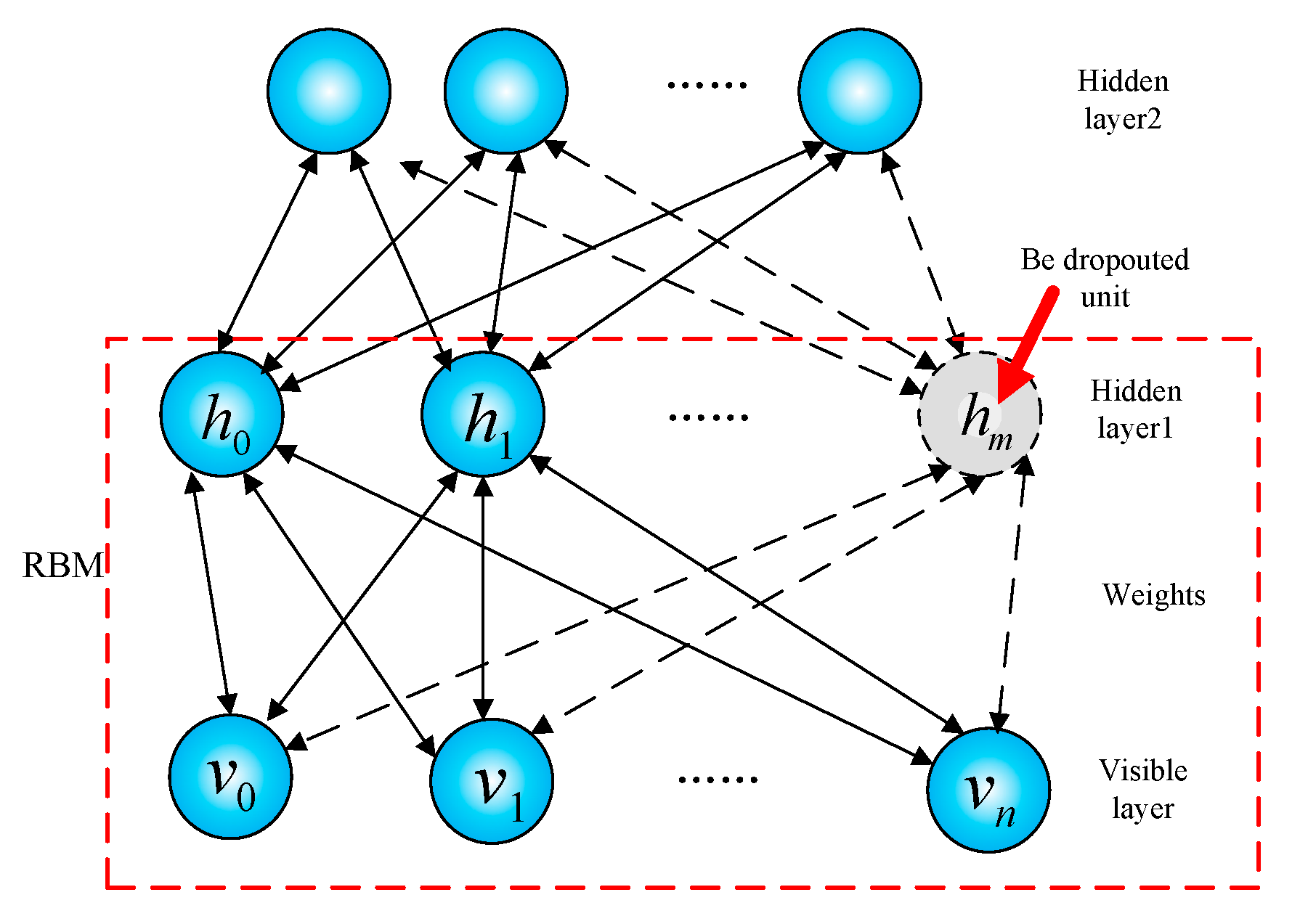
Send the data to the input layer and start training the first RBM. Perform dropout to determine which feature detectors can be removed according to Equations (5) and (6) and use the remaining neurons to conduct the feature extraction.
(3)
Use the CD algorithm to quickly train an RBM and use Equations (7) and (8) to perform the data calculation. Reduce overfitting and improve computational efficiency by introducing the regularization enhancement factor.
(4)
Update the RBM network parameters.
(5)
Use the RBM output as the input of the next RBM and perform the same process on the next RBM.
(6)
When the last RBM is trained, perform the next step to output the data; otherwise, return to Step (2).
(7)
Use the backpropagation algorithm to conduct supervised training.
(8)
If the training termination conditions are met, stop training; otherwise, go back to Step (7).
(9)
Stop the operation.
The RBM pseudocode for unsupervised training is listed below. The software used is MATLAB, the experiments are run on a computer with 64 GB memory, 1024 GB hard disk, no GPU is installed. The code we are using is an open source downloaded from online, and we have modified it for our own purpose [24].

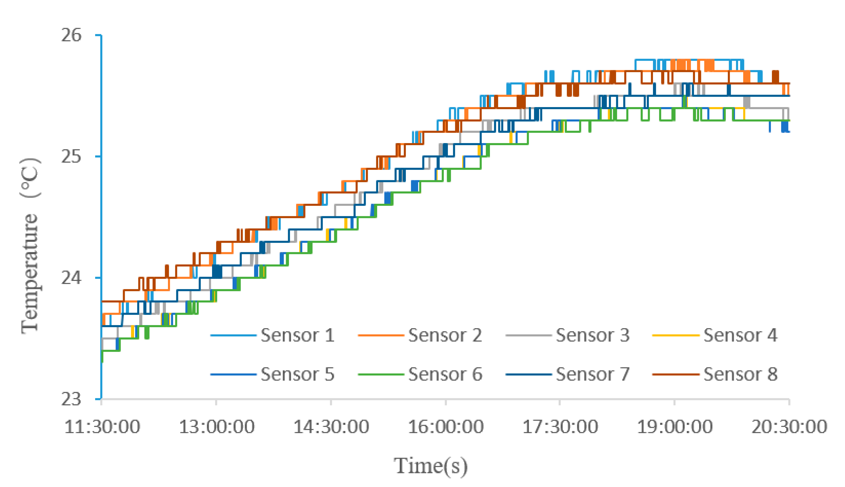
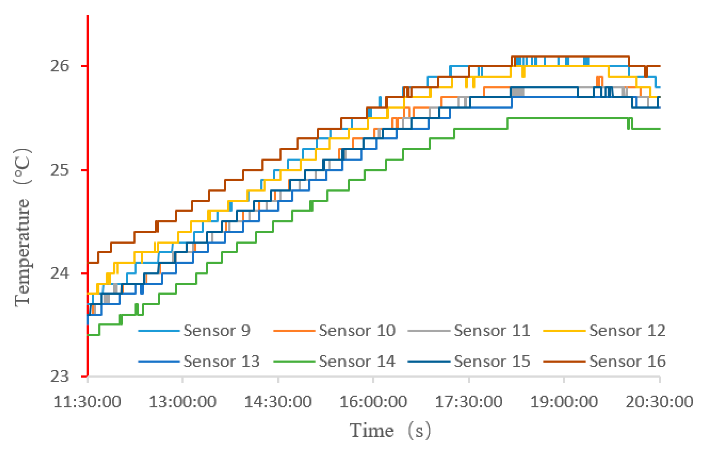
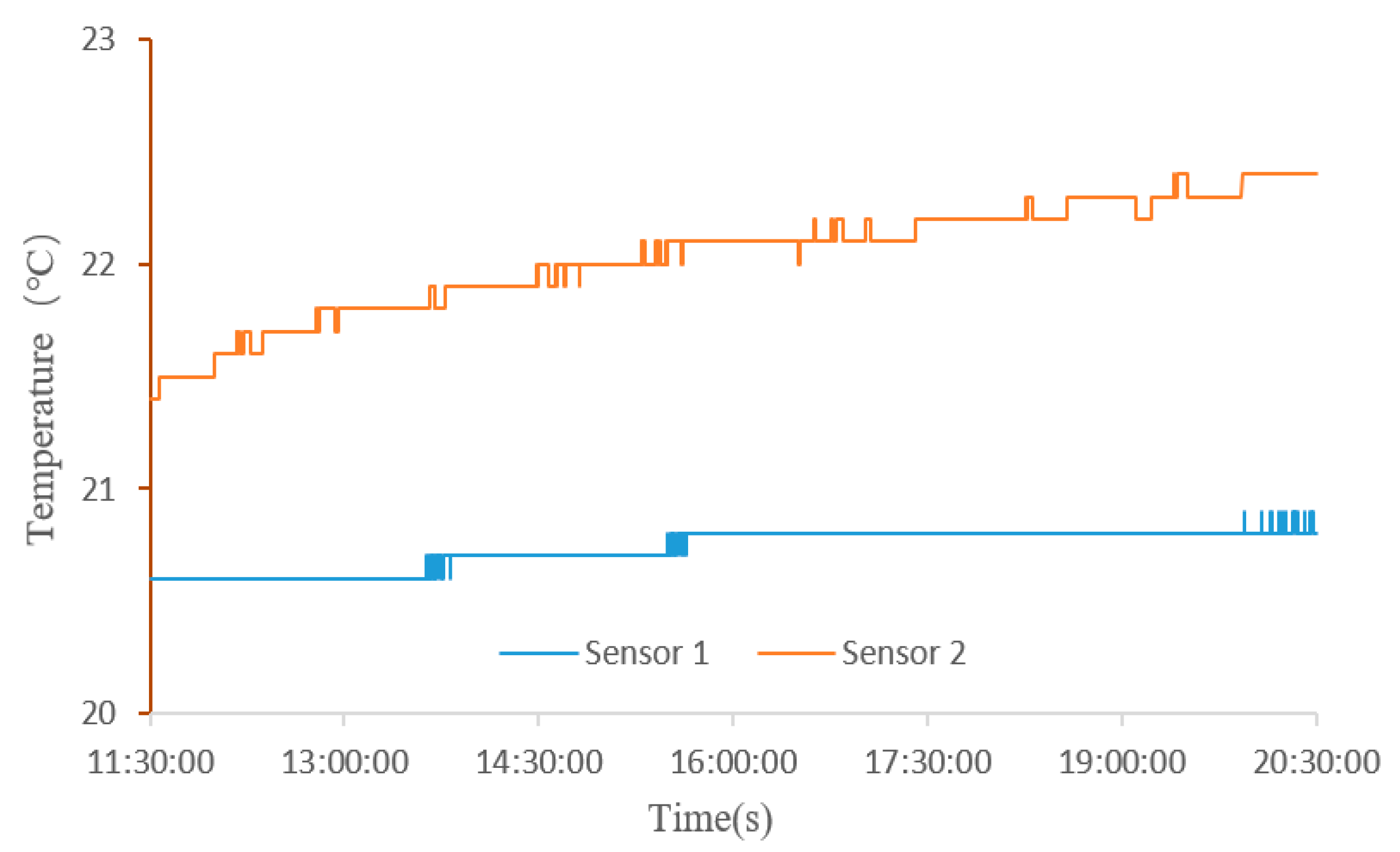
3.2. Acquisition of Experimental Data

In order to train an AI model, experimental measurement on thermal errors is must performed, because the weights of AI model are random before training, and the model needs to “watch and learn” enough real data to help it to adjust weights. Once the model is trained, it can calculate thermal errors on new data. Since heavy-duty machine tools have large heat exchange surfaces, uneven ambient temperature distribution and temperature fluctuations could cause considerable changes to the spatial posture of the machine. Whether the temperature changes are a result of the shift from one season to another or from day to night, temperature changes can seriously affect the precision of the machining process. For heavy duty machine tools up to dozens of meters high, the temperature gradient in the ambient environment is important. In addition, because some workshops are temporarily reconstructed, their working environment is even worse, for example, there are a large range of glass windows in the workshop. Thus, measuring the ambient temperature from a single location—the practice adopted for most machine tools—does not suit heavy-duty machine tools. In addition, the heat of hydration of cement, changes in ambient temperature, and other factors can cause thermal error of the reinforced concrete foundations of heavy-duty machine tools. Therefore, when studying the thermal error of machine tools caused by changes in ambient temperature, the heat coupling effects between the superstructure and foundation should be fully considered. To address this, a monitoring system is proposed for monitoring the thermal error of heavy machine tool-foundation systems.

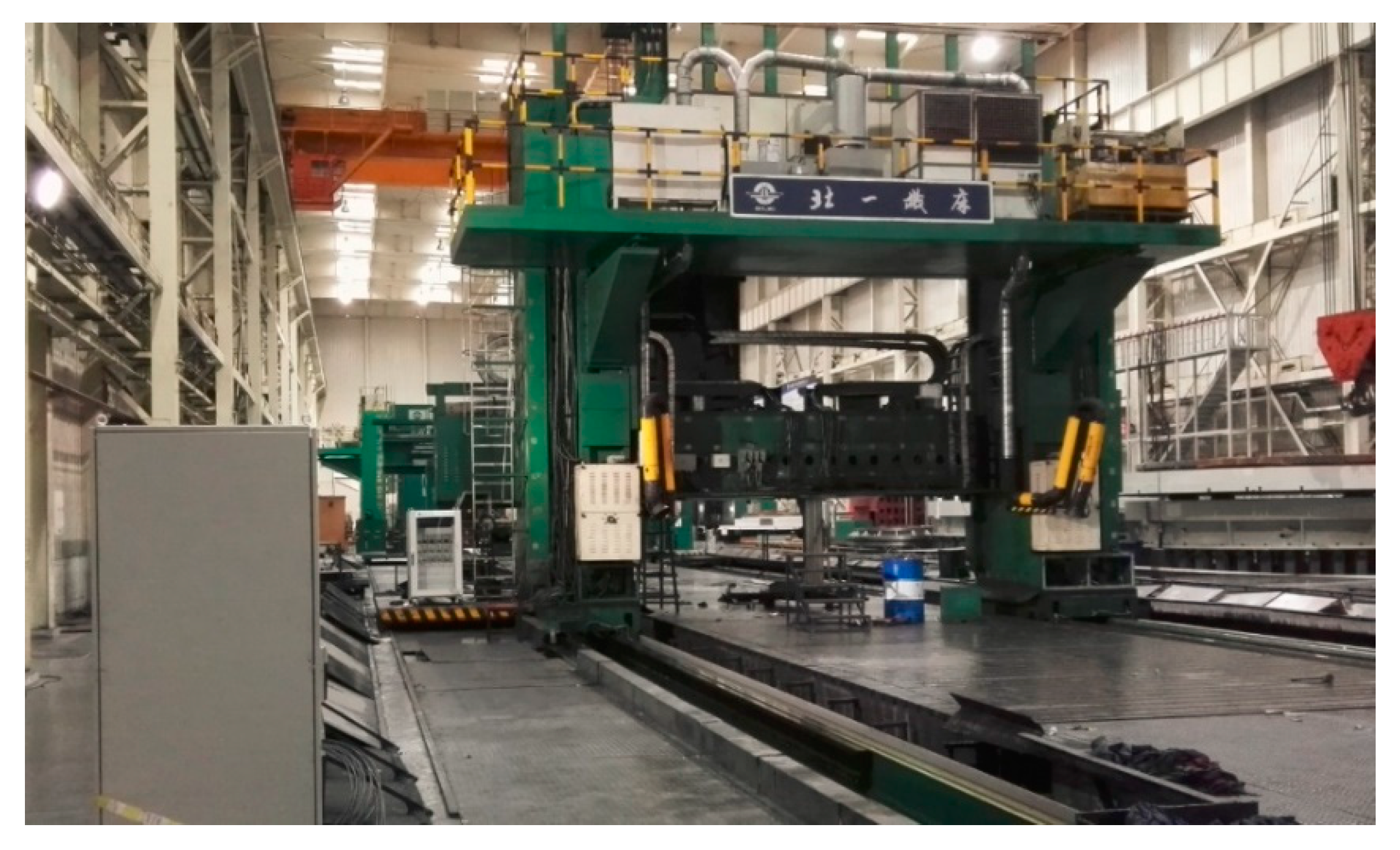
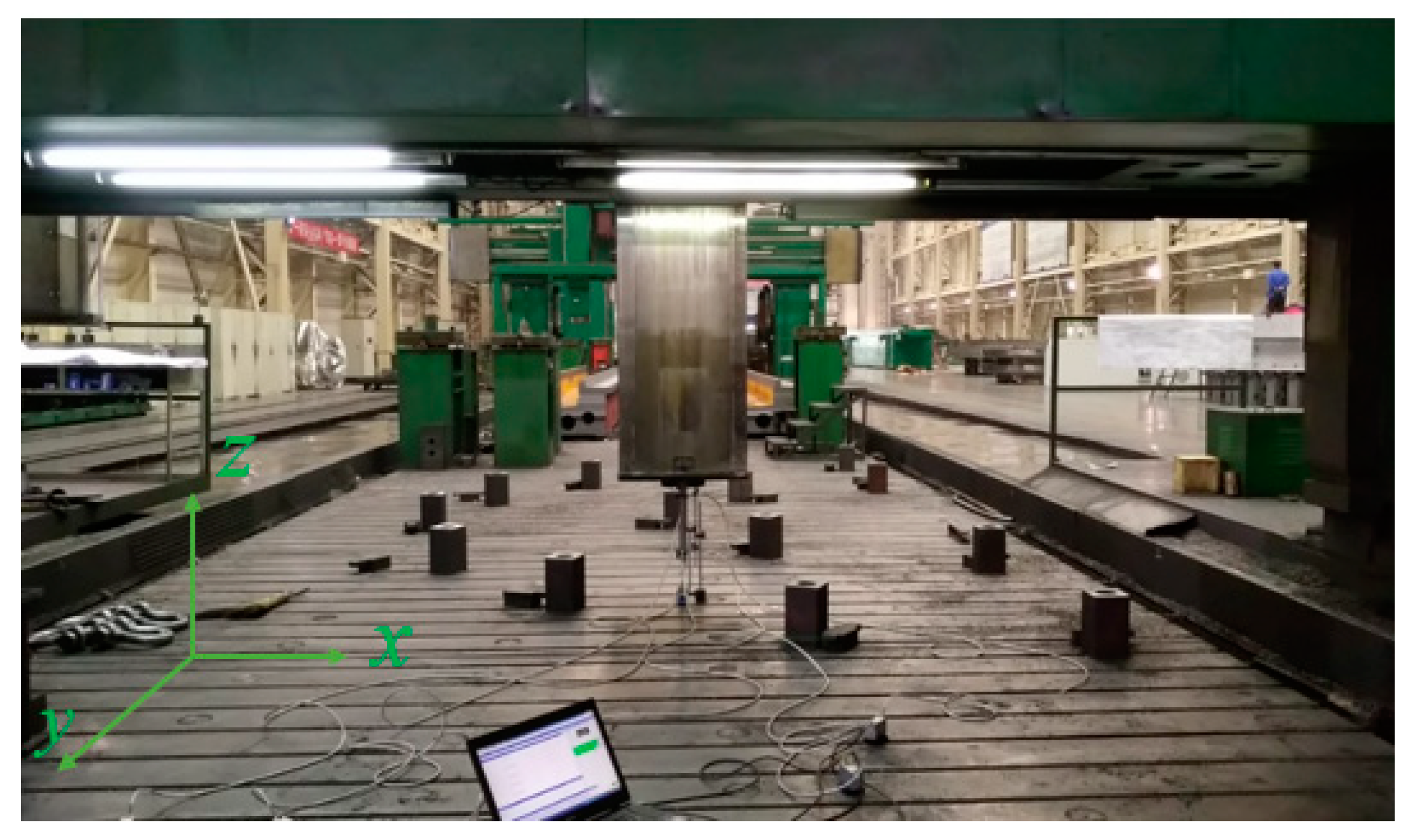
3.2.1. Experimental Environment

The object used in this study was a heavy-duty CNC machine tool. The machine tool has a width of 9.7 m and height of 8.5 m and the dimensions of the concrete foundation are 57 m × 17 m × 7 m (length × width × height). The ambient environment was a workshop in Shunyi District, Beijing City with ceiling lights and no glass windows. The door of the workshop was located 15 m from the closest end of the machine tool and all other factory operations were halted during the experiment. There was no vibration in the surrounding environment. The experiment was carried out in April of 2019 and the indoor temperature difference was 3–4 °C (Figure 3).

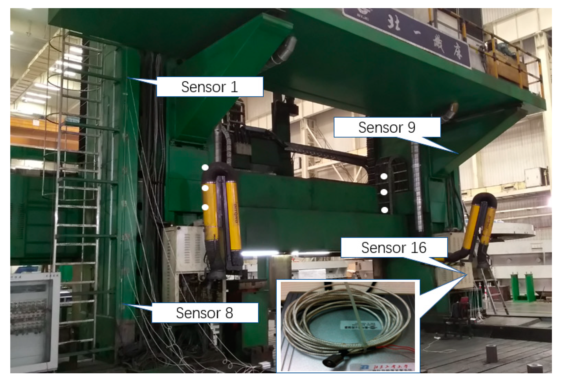
3.2.2. Deployment of Sensors

According to the structure and size characteristics of the experimental machine tool, a temperature sensor is arranged every 0.8 m in the column, and a total of 16 temperature sensors are arranged on the left and right sides. In addition, one sensor is arranged every 0.8 m in the vertical direction in the concrete foundation, and two temperature sensors are arranged in total (Figure 4). Sensor model: PT100 magnetic temperature sensor, measuring range: −20~100 °C, accuracy is 0.1 °C. If the change of temperature is in 0.01 °C level, the change of thermal error is relatively small, so, it the sensors that are used should be accurate enough.
To measure the effects of ambient temperature changes caused by opening and closing the workshop door on the thermal error of the spindle, the machine was turned off for two days before the experiment to ensure no heat was generated by the machine. In order to realize the synchronous acquisition of thermal error data, the mandrel is installed in the experiment process, and the eddy current sensor is installed at the bottom of the mandrel, so as to collect the displacement data in Z direction in real time (Figure 5).

4. Comparison of Predicted Values and Experimental Results

Firstly, as discussed, experimental data (training data and the corresponding thermal errors) should be measured. The ability of feature learning is an inherent characteristic of the proposed model, and one of the most observable outward manifestations is model’s performance on predicting outputs based on given inputs. In the experiment, two sets of thermal error data and temperature data for the heavy-duty machine tool-foundation system were collected. The first set of data was used to establish the thermal error predictive model. The second was used to verify the accuracy of the predictive model. During the experiment, the collected data is divided into two parts: the first part is 11:30–19:30 data (training data), the second part is 19:30–20:30 data (test data). 32,400 experimental data are obtained for each sensor by setting 1 s sampling period of temperature and displacement data. We used 18 temperature values and one displacement value at the same time constitute a sample, so a total of 32,400 experimental samples during the 9-h data collection process. Figure 6, Figure 7 and Figure 8 show the temperature changes at the measurement locations on the columns of the machine tool and the concrete foundation.
It can be seen from Figure 6 and Figure 7 that the highest temperature occurs at around 7 PM, and significantly lags behind the highest outdoor temperature (the highest outdoor temperature appears around 2 PM in this season). The temperature difference between 11:30 and 20:30 is 2.5 °C. There is a temperature gradient in the vertical direction of the machine tool and the temperature decreases with height. Figure 8 shows that temperature differences the concrete foundation are larger than those of the superstructure. The variation of temperature with time can clearly be observed. It should be noted that Figure 6, Figure 7 and Figure 8 shows data collected by several sensors. In an ideal scenario, the temperature difference between the two sensors is always a constant (if so, the coordinate offset could be easily obtained using Figure 9). However, the external environment (opening and closing doors of workshop, etc.) makes it inconstant. Besides, the change of seasons also has effect on temperature difference. As a result, temperature measured by a sensor at a certain moment could be independent and changeable, and the thermal error cannot be obtained simply using Figure 9. Therefore, in order to obtain accuracy values in reality, people have to find another way to model the accuracy value. That is why deep neural network is proposed as an alternative. In the experiment, in order to train a model with high robustness, all the data in training a neural network model should be obtained one by one by human-labor.
This paper focuses on the thermal error caused by the environment temperature. The results show that the thermal error caused by the ambient temperature is mainly concentrated in the Z direction, and the error in other directions is rather small (the largest error in the other direction occurs in the x direction, which is only 7.6% of the error in the Z direction). Therefore, thermal error in the Z direction is predicted by temperature value as input. Because there are some noises in the collected data, this paper uses the integral differential Jacobian polynomial method to reduce the noise of the collected displacement data [25]. Actually, the training data is not related to time, because the temperature is changed with the change of sensors’ location, and that is how we collect a new set of training data. The thermal error is collected by the displacement sensor at 11:30, so the thermal error caused by heat is 0 in the initial stage, and the subsequent errors are relative to the initial time. Figure 9 shows thermal error in the z-direction of the spindle terminal as it relates to changes in ambient temperature.
In this study, different thermal error predictive models were used to predict the thermal error of the machine tool, and the models were compared to decide which one was better in terms of prediction accuracy. This paper divides the second set of the test data into 10 groups and predicts them. Predictions based on different thermal error models were obtained. In order to verify the overall performance of the self-organizing DNN network modeling method, two types of network were used at the same time to train the model using thermal error data. Performances of the predictive models are compared in Figure 10.
To compare the generalization ability, for all cases, epochs were given a value of 200 and supervised training was performed for 1000 steps. Under the same experimental conditions, the root mean square error of the self-organizing DNN was lower than that of the DNN, which suggests the self-organizing DNN provides more accurate predictions of the thermal error and has better generalization ability. Self-organizing DNN achieved a convergence speed much higher. Under the same experimental conditions, the overall training time was longer than 6 h, and it took each RBM approximately 1 h to complete the unsupervised training. Since the self-organizing DNN uses a self-organizing mechanism to randomly remove neurons and the regularization enhancement algorithm also has an influence on the convergence rate of unsupervised training, the training time of each RBM was 2–3 h, which is an improvement of more than 30%. Experiments show that self-organizing DNN has a faster convergence speed and better generalization ability under the same neural network structure and experimental conditions. A comparison of data in the second and third curve of Figure 10 reveals that both the drop rate and regularization enhancement parameter have an influence on the training results. Appropriately increasing the values of the drop rate and performance parameters will improve the accuracy of the model, however further increases will lead to increased training error. Thus, choosing a proper drop rate value is important as well as trying different performance parameter values during different experiments. When the network is applied to the multitasking problem, a larger network structure may be required and the drop rate and regularization enhancement parameter should be adjusted for different values based on different experiments. By comparing the mean squared error (MSE) of each method, we can see that: The prediction result of self-organizing DNN (alpha = 0.8, beta = 0.2) has the lowest error and is more stable. One should note that the training data is not too much in this experiment, this is because not all conditions are considered and tested. For example, if the workshop door opens often in winter, the measured temperature will be changed greatly, which may cause thermal error harder to predict. This is what we will continue in next step. However, in this paper, we have fully trained and tested the model using current dataset. For example, many different training parameters (unsupervised training steps, supervised training steps, learning rates, hidden layer neuron number, etc.) are evaluated, and the best parameter is selected. Moreover, the model is trained and tested for several times, to evaluate the stability. In the future, we believe that the method is easily applied to other conditions based on the current research.

5. Conclusions

(1)
In this study, a thermal error prediction model has been developed based on self-organizing DNN with the aim of improving feature extraction capabilities, reducing test errors, and improving convergence speed. The dropout mechanism was used to train the self-organizing capability of the hidden layer during unsupervised training of the neural network, thereby preventing synergy between neurons in the same layer and improved the feature extraction capability. Furthermore, a regularization enhancement factor was introduced into the training objective function to prevent overfitting and reduce training times.
(2)
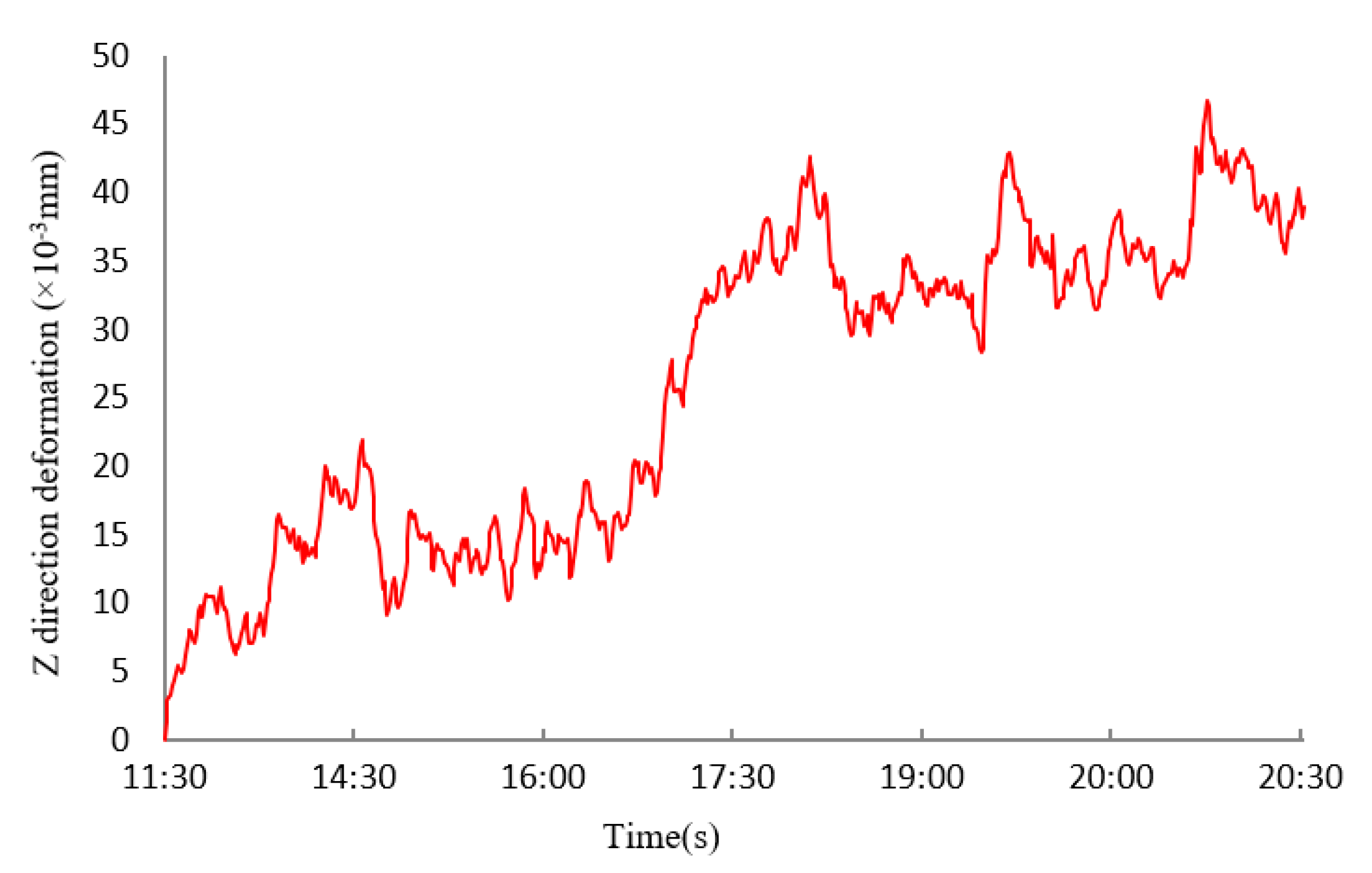
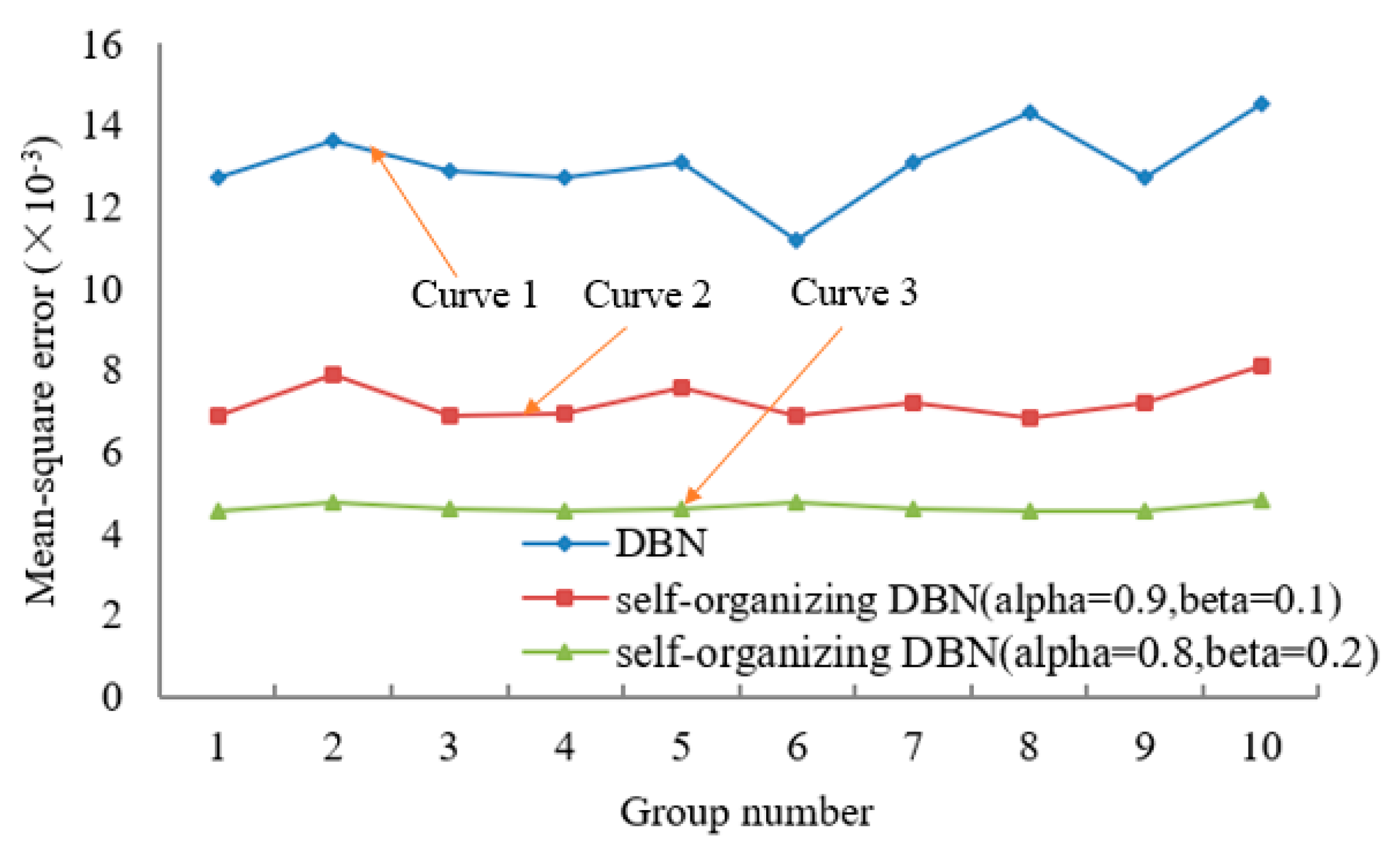
The effects of ambient temperature changes on thermal error of the machine tool-foundation system was analyzed within a 9-h timeframe based on experimental data. A comparison of the prediction results of self-organizing DNN and traditional DNN revealed that the self-organizing DNN network predictive model proposed in this paper has better generalization ability and higher convergence speeds, moreover, adjusting the drop rate improves the overall predictive capability of the network. Moreover, because the machine’s environment and construction are different, if we want to transfer the trained model on other machines (or new testing environments), new training data must be collected, and the model must be re-trained or fine-tuned. So, the trained model is not universal, because it is only trained for the particular experiment. However, the methodology that we proposed in the paper is totally original and universal, we believe if more data could be collected in various conditions, a model with universal power could be trained.

Author Contributions

Conceptualization, Y.T.; methodology, Y.T. and G.P.; validation, Y.T.; formal analysis, G.P.; data curation, Y.T.; writing—original draft preparation, Y.T. and G.P.; supervision, G.P.; project administration, Y.T.; funding acquisition, Y.T. All authors have read and agreed to the published version of the manuscript.

Funding

This work was supported by the Scientific Research Fund of Department of Education of Liaoning Province, China (LG201926), Shenyang Young and Middle-aged Science and Technology Innovation Talents Support Fund (RC180185).

Acknowledgments

The authors gratefully acknowledge the anonymous reviewers for their careful reading and useful comments that allowed to improve the quality of this paper.

Conflicts of Interest

The authors declare no conflict of interest.

References

  1. Tan, B.; Mao, X.; Liu, H.; Li, B.; He, S.; Peng, F.; Yin, L. A thermal error model for large machine tools that considers environmental thermal hysteresis effects. Int. J. Mach. Tools Manuf. 2014, 82, 11–20. [Google Scholar]
  2. Mian, N.S.; Fletcher, S.; Longstaff, A.P.; Myers, A. Efficient estimation by FEA of machine tool distortion due to environmental temperature perturbations. Precis. Eng. 2013, 37, 372–379. [Google Scholar]
  3. Pahk, H.; Lee, S.W. Thermal Error Measurement and Real Time Compensation System for the CNC Machine Tools Incorporating the Spindle Thermal Error and the Feed Axis Thermal Error. Int. J. Adv. Manuf. Technol. 2002, 20, 487–494. [Google Scholar] [CrossRef]
  4. Wang, H.; Wang, L.; Li, T.; Han, J. Thermal sensor selection for the thermal error modeling of machine tool based on the fuzzy clustering method. Int. J. Adv. Manuf. Technol. 2013, 69, 121–126. [Google Scholar]
  5. Yang, H. Dynamic modeling for machine tool thermal error compensation. J. Manuf. Sci. Eng. 2003, 125, 245–254. [Google Scholar] [CrossRef]
  6. Wang, Y.; Zhang, G.; Moon, K.S.; Sutherland, L.W. Compensation for the thermal error of a multi-axis machining center. J. Mater. Process. Technol. 1998, 75, 45–53. [Google Scholar]
  7. Kang, Y.; Chang, C.W.; Huang, Y.; Hsu, C.L.; Nieh, I.F. Modification of a neural network utilizing hybrid filters for the compensation of thermal deformation in machine tools. Int. J. Mach. Tools Manuf. 2007, 47, 376–387. [Google Scholar]
  8. Li, F.; Li, T.; Wang, H.; Jian, Y. A Temperature Sensor Clustering Method for Thermal Error Modeling of Heavy Milling Machine Tools. Appl. Sci. 2017, 7, 82. [Google Scholar]
  9. Chen, J.S.; Yuan, J.X.; Ni, J. Thermal error modeling for realtime compensation. Int. J. Adv. Manuf. Technol. 1996, 12, 266–275. [Google Scholar] [CrossRef] [Green Version]
  10. Lee, D.S.; Choi, J.Y.; Choi, D.H. ICA based thermal source extraction and thermal distortion compensation method for a machine tool. Int. J. Mach. Tools Manuf. 2003, 43, 589–597. [Google Scholar] [CrossRef]
  11. Guo, Q.; Yang, J.; Wu, H. Application of ACO-BPN to thermal error modeling of NC machine tool. Int. J. Adv. Manuf. Technol. 2010, 50, 667–675. [Google Scholar] [CrossRef]
  12. Zhang, Y.; Yang, J.; Jiang, H. Machine tool thermal error modeling and prediction by grey neural network. Int. J. Adv. Manuf. Technol. 2012, 59, 1065–1072. [Google Scholar] [CrossRef]
  13. Wang, L.; Wang, H.; Li, T.; Li, F. A hybrid thermal error modeling method of heavy machine tools in z -axis. Int. J. Adv. Manuf. Technol. 2015, 80, 389–400. [Google Scholar]
  14. Gomez-Acedo, E.; Olarra, A.; de la Calle, L.N.L. A method for thermal characterization and modeling of large gantry-type machine tools. Int. J. Adv. Manuf. Technol. 2012, 62, 875–886. [Google Scholar] [CrossRef]
  15. Lee, S.K.; Yoo, J.H.; Yang, M.S. Effect of thermal deformation on machine tool slide guide motion. Tribol. Int. 2003, 36, 41–47. [Google Scholar] [CrossRef]
  16. Liu, Q.; Yan, J.; Pham, D.T.; Zhou, Z.; Xu, W.; Wei, Q.; Ji, C. Identification and optimal selection of temperature-sensitive measuring points of thermal error compensation on a heavy-duty machine tool. Int. J. Adv. Manuf. Technol. 2016, 85, 345–353. [Google Scholar]
  17. Gomez-Acedo, E.; Olarra, A.; Zubieta, M.; Kortaberria, G.; Ariznabarreta, E.; de la Calle, L.N.L. Method for measuring thermal distortion in large machine tools by means of laser multilateration. Int. J. Adv. Manuf. Technol. 2015, 80, 523–534. [Google Scholar] [CrossRef]
  18. Kogbara, R.B.; Iyengar, S.R.; Grasley, Z.C.; Rahman, S.; Masad, E.A.; Zollinger, D.G. Correlation between thermal deformation and microcracking in concrete during cryogenic cooling. NDT E Int. 2016, 77, 1–10. [Google Scholar]
  19. Lee, J.H.; Kalkan, I. Analysis of Thermal Environmental Effects on Precast, Prestressed Concrete Bridge Girders: Temperature Differentials and Thermal Deformations. Adv. Struct. Eng. 2012, 15, 447–460. [Google Scholar] [CrossRef]
  20. Hinton, G.E. Reducing the Dimensionality of Data with Neural Networks. Science 2006, 313, 504–507. [Google Scholar] [CrossRef] [Green Version]
  21. Hinton, G.E.; Srivastava, N.; Krizhevsky, A.; Sutskever, I.; Salakhutdinov, R.R. Improving neural networks by preventing co-adaptation of feature detectors. Comput. Sci. 2012, 3, 212–223. [Google Scholar]
  22. Tian, Y.; Liu, Z.; Cai, L.; Pan, G. The contact mode of a joint interface based on improved deep neural networks and its application in vibration analysis. J. Vibroeng. 2016, 18, 1388–1405. [Google Scholar]
  23. Rumerlhar, D.E. Learning representation by back-propagating errors. Nature 1986, 323, 533–536. [Google Scholar]
  24. Available online: www.deeplearning.net (accessed on 15 April 2020).
  25. Liu, D.Y.; Gibaru, O.; Perruquetti, W. Differentiation by integration with Jacobi polynomials. J. Comput. Appl. Math. 2011, 235, 3015–3032. [Google Scholar] [CrossRef] [Green Version]
Figure 1. Structure of self-organizing deep neural network (DNN).
Applsci 10 02870 g001
Figure 2. Dropout in unsupervised training.
Applsci 10 02870 g002
Figure 3. Working environment.
Applsci 10 02870 g003
Figure 4. Overview of the sensor deployment scheme.
Applsci 10 02870 g004
Figure 5. Data acquisition of thermal error.
Applsci 10 02870 g005
Figure 6. The temperature changes at the measurement locations on the left column.
Applsci 10 02870 g006
Figure 7. The temperature changes at the measurement locations on the right column.
Applsci 10 02870 g007
Figure 8. The temperature changes at the measurement locations the concrete foundation.
Applsci 10 02870 g008
Figure 9. Thermal error in the z-direction of the spindle.
Applsci 10 02870 g009
Figure 10. Comparing different methods.
Applsci 10 02870 g010

