Article

ConvProtoNet: Deep Prototype Induction towards Better Class Representation for Few-Shot Malware Classification

1
College of Software Engineering, Sichuan University, Chengdu 610000, China
2
College of Cybersecurity, Sichuan University, Chengdu 610000, China
3
College of Computer Science, Sichuan University, Chengdu 610000, China
*
Author to whom correspondence should be addressed.
Appl. Sci. 2020, 10(8), 2847; https://doi.org/10.3390/app10082847
Submission received: 29 February 2020 / Revised: 13 April 2020 / Accepted: 14 April 2020 / Published: 20 April 2020

Abstract

:
Traditional malware classification relies on known malware types and significantly large datasets labeled manually which limits its ability to recognize new malware classes. For unknown malware types or new variants of existing malware containing only a few samples each class, common classification methods often fail to work well due to severe overfitting. In this paper, we propose a new neural network structure called ConvProtoNet which employs few-shot learning to address the problem of scarce malware samples while prevent from overfitting. We design a convolutional induction module to replace the insufficient prototype reduction in most few-shot models and generates more appropriate class-level malware prototypes for classification. We also adopt meta-learning scheme to make classifier robust enough to adapt unseen malware classes without fine-tuning. Even in extreme conditions where only 5 samples in each class are provided, ConvProtoNet still achieves more than 70% accuracy on average and outperforms other traditional malware classification methods or existed few-shot models in experiments conducted on several datasets. Extra experiments across datasets illustrate that ConvProtoNet learns general knowledge of malware which is dataset-invariant and careful model analysis proves effectiveness of ConvProtoNet in few-shot malware classification.

1. Introduction

Malware is defined to be all programs that can incur computer crash, privacy leak, illegal invasion, resource damage, and so on. Malware has become one of the most effective threats in cyber world: Reported in Kaspersky Security Bulletin 2019, 24 million of unique malwares were detected and 19.8% of user computers were attacked in 2019. According to their working mechanisms, they can be classified into many families or variations like Virus, Worm, Trojan, Backdoor, Rootkit, etc. [1] and they are analyzed carefully to develop countermeasures after classification. However, new variants of malware can appear rapidly and a detected malware type can fool the classifier by deriving a variant using encryption, packing, polymorphism, ob-fuscation, and meta-morphism techniques [2].
Most of malware classification uses machine learning methods such as Support Vector Machines (SVM), decision trees, logistic regression, etc. to classify malwares after extracting malware features such as n-gram. Deep learning models, such as Multi-Layer Perceptron (MLP), Convolutional Neural Network (CNN) and Recurrent Neural Network (RNN) were also explored to do malware classification and achieved great accuracy [3,4,5]. However, most above methods can only work well when a large amount of labeled data are available to run supervised learning algorithm. When it comes to a rare variant or a newly detected malware type, lacking data can lead to severe overfitting or convergence problem and we are not able to forewarn these malwares before they are spread and cause serious damage. Moreover, collecting malware samples is a laborious and time-consuming work which will block the research on a new type of malware.
To address these problems, we introduce few-shot learning to malware classification which allows model to learn general and high-level knowledge of malware over a series of similar tasks and task-specific information is extracted from a few samples to adapt unseen classes during training [6,7]. Using few-shot learning can solve the problem of limited data and alleviate the fatigue of manual malware labeling. Despite being commonly discussed in image classification [8,9,10,11,12], character recognition [8,9,13] and text classification [14,15] tasks, few-shot learning cannot be directly applied to malware which contains complex structured information and we adopt the approach proposed by Nataraj et al. [16] to convert malware to images that are easier to process. Using malware images instead of original samples can minimize the need for expert knowledge of malware classification while keep the integrity of information in malware. As shown in Figure 1, malware images from the same class tend to have similar textures.
There are some shortcomings to employ existing few-shot models in malware classification. Many few-shot learning models use embedding-based methods that embed samples in embedding space and reduce the samples in the same class to a class prototype where classification is done by comparing the distances between sample and different class prototypes. However, many reduction algorithms used in few-shot models only compute the shallow prototypes such as mean to represent the latent unknown class distribution [9,14] and the performance of malware classification may degrade if we use these insufficient class prototypes to classify newcome malwares. Most embedding-based few-shot models adopt an inherited structure of embedding function called Conv-4 which extracts less comprehensive features [8,9,14]. To make matter worse, some designs in few-shot models like distance attention may give rise to gradient vanishing and decelerate the learning procedure [15].
In this paper, we propose a new model called ConvProtoNet to solve above problems and boost the performance of malware few-shot classification. Unlike simply computing mean, we use stacked convolution layers to generate high-level malware class feature and the output of this structure serves directly as malware class prototypes used to classify new malwares instead of distance attention to avoid gradient vanishing. Also, we enrich representation of features by removing Rectified Linear Unit (ReLU) activation and perform Channel Pooling to allow adaptive input sizes for flexibility. ConvProtoNet is trained by episode-based meta learning strategy end-to-end. After training, the parameters in ConvProtoNet are shared by all malware few-shot classification tasks and new tasks can be solved without fine-tuning. It is worth noting that ConvProtoNet can be trained on a single malware dataset and work on another malware datasets as well as achieving considerable performance. This shows the strong generalization ability of ConvProtoNet.

2. Related Work

2.1. Malware Classification

Traditional malware analysis is often divided into static and dynamic analysis. Static analysis only makes use of raw byte features or disassembled instruction sequences without really executing malware. These static features include byte N-Gram distribution or Term Frequency and Inversed Document Frequency (TF-IDF) [17,18,19,20], Application Programming Interface (API) call sequence [21], opcode N-Gram [22], control flow graph(CFG) [2,19], function length frequency(FLF) [23] and printable string information (PSI) [23,24] etc. Static analysis features are cheap and fast to obtain, but they can be easily confused by variants of malware using encryption, packing, polymorphism, obfuscation, meta-morphism techniques [2]. Dynamic analysis methods collect behaviors of malware when executing in virtual environment that reflect their run-time intent [1,2,25]. Dynamic analysis can be more accurate but more time-consuming and costly than static analysis limiting their large-scale application. Dynamic techniques include function call monitoring, function parameter analysis, information flow tracking, instruction traces, autostart extensibility points and so on [1]. After analysis, common machine learning tools are utilized to build classification model including SVM, decision tree, Naïve Bayes, Decision Tree, Boosted Tree, k-Nearest-Neighbor(kNN) etc. discussed in [25].
Typically, Abou-Assaleh et al. [17] used Common N-Gram Analysis (CNA) extracting distribution of N-Gram substrings of malware as input and kNN algorithm as classification method where only most frequent N-Gram substrings take effect. Santos et al. [20] also extracted N-Gram statistic as input but made some changes when calculating sample-wise distance. Bhodia et al. [26] chose to extract PE meta-data instead of raw-byte features and similarly used kNN to classify.

2.2. Malware Image

Nataraj et al. first proposed the concept of malware image which converts raw-byte malware PE files to gray-scale images [16] and they employed GIST descriptor [27] to extract global image properties as input features to kNN. Malware images can retain global structure even if some small changes occur [28] and minimize the need of expert knowledge [3]. Liu et al. [29] also made use of malware image but they calculated local mean of image from disassembled file for reduction. Recently, an increasing number of contemporary methods using malware image to classify turn to employ deep learning models like CNN due to their powerful extraction ability, resistance to noise and robustness when processing different modalities of data [3,28,30,31]. VGG-based and ResNet-based advanced architectures are also exploited [26,32,33,34]. Differently, Vu et al. [35] developed a novel approach using hybrid transformation to convert malware to color images that convey malware semantics to perform malware classification tasks.

2.3. Few-Shot Learning

Few-shot learning (FSL) [7] aims to recognize novel classes where a few samples are available. FSL does not learn a fixed task during training but learn on a set of similar tasks from a task distribution. Embedding-based methods are popular among few-shot learning approaches which typically project input to embedding space so that similar and dissimilar samples can be easily discriminated. Generally, embedding function is learned in a task-invariant manner so that task-specific information can be quickly assimilated by feeding samples without retraining. Koch [13], Sung et al. [8] and Vinyals et al. [36] made pair-wise comparisons which is equivalent to do kNN in embedding space. To reduce the influence of noisy samples, many models extract class prototypes from a few samples to replace the kNN with the nearest neighbor classification between the queried sample and class prototypes, for instance Prototypical Network proposed by Snell et al. [9] which computes mean as class prototypes and classifies according to square Euclidean distance. Geng et al. [14] used dynamic routing algorithm to obtain class prototypes and Gao et al. proposed Hybrid Attention-Based Prototypical Network [15] referring to attention mechanism to compute prototypes so as to suppress noise. Some other work such as Gidaris et al. [10] and Qi et al. [11] can be viewed as extensions of above embedding-based work.
Many researches tried to solve few-shot learning in other perspectives. MAML proposed by Finn et al. [37] is a general training strategy trying to offer good initial value to fine-tune and fast adaption to target tasks. Simple neural attentive learner (SNAIL) [38] is also a general few-shot learning framework using causal convolution and attention mechanism. Like MAML, Meta-SGD [39] offers good initial value and it can adaptively adjust the step direction and step length using a parameterized term controlling the gradient. Long Short-Term Memory (LSTM) meta learner proposed by Ravi et al. [12] trains a LSTM-based meta learner to output optimization steps at each iteration. Meta Network proposed by Munkhdalai et al. [40] allows fast generalization through shift of inductive bias using meta learner. Besides, lots of researchers try to generate auxiliary samples using a few samples in a class to alleviate overfitting [41,42,43] where Generative Adversarial Network (GAN) is commonly used. Generating process called hallucination is often guided by attribute, semantics and regularization to reduce deviation between results and original samples. However, hallucination-based methods are difficult to implement where quality of hallucinated data is hard to guarantee.

3. Method

3.1. Problem Definition

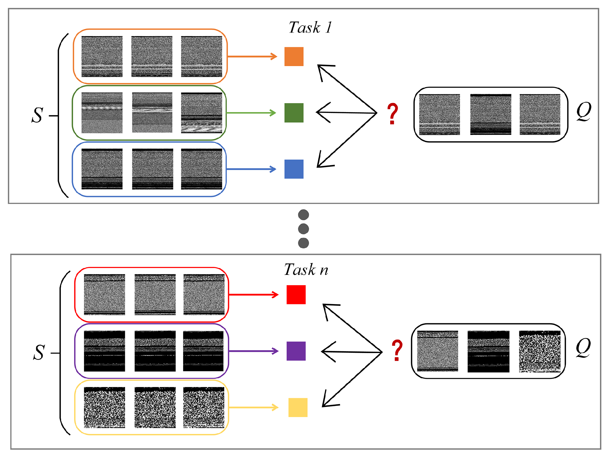
In this paper, we primarily focus on few-shot classification task on malware datasets where new classes that are not observed during training must be accommodated given only a few samples each class. A large dataset containing many classes but not many samples per class is split to two parts called meta-training set D t r a i n and meta-testing set D t e s t respectively and class labels in two sets are made disjoint. Each classification task on meta-training set or meta-testing set both consist of a support set S (observed for model) and a query set Q (not observed for model) sharing the same label space. For each task, possible classes are different and our model must classify samples in Q where only S is provided, as shown in Figure 2. We adopt prototype-based classification scheme as in [9] where each class owns a class prototype reduced from samples in class.
Typically, there are K samples for a class in S provided for training (K is usually small, e.g.,  K = 5 ), and N samples per class in Q used for testing generalization ability. To follow the naming convention of FSL, we define the basic task that classifies samples in Q based on K labeled samples in S into C classes to be a K-shot C-way task. In training stage, only D t r a i n is available and D t e s t is used in testing stage to test the performance of model when adapting to unseen classes.

3.2. Training Strategy

To ensure minimum performance and make fair comparison with other models, we take episode-training used in [8] on meta-training set to mimic meta-testing stage to make training procedure match testing procedure. A training episode is constructed by first randomly selecting C classes from D t r a i n to form the label space L. Then, K and N samples of each selected class are taken out from D t r a i n to put into S and Q respectively where S = ( x i S , y i S ) i = 1 K × C and Q = ( x i Q , y i Q ) i = 1 N × C are kept non-overlapped.
At each training iteration, an episode (task) is sampled from an implicit task distribution T as above and S is fed into model to provide task information where a task-specific classifier c ^ ( S ) is generated. Class prototypes are contained in c ^ ( S ) and classification of queried samples is completed by comparing with class prototypes. After that, Q is input to c ^ ( S ) producing loss of this task by loss function L . Model parameter ϕ is updated according to the loss in Q:
ϕ = arg min ϕ E L T E S , Q L i L ( y i Q , x i Q | S , ϕ ) .
It should be noted that, diversity of tasks must be ensured to simulate the task distribution which requires enough classes in D t r a i n and more training iterations than common models to obtain an ideal result. Thanks to exponential growth of possible tasks with the class amount, there are great amount of available combinations of task to prevent from overfitting caused by lack of samples. More precisely, when there are M classes in D t r a i n , we can have C M possible tasks, which is also mentioned in [14].

3.3. Conversion from Malware to Images

Although some previous work used malware images in rectangle shape with fixed width and variable height [26], instead we use square images in fix size 256 × 256 for batch integration purpose. In our implementation, malware as byte sequences will first be reshaped to square gray scale images. Then, up-sampling or down-sampling techiniques will be applied on square images to fit the size of 256 × 256 . This process is described in detail in Algorithm 1. Our method is kind of similar to the one in [44], and some information like tail bytes in malware will be dropped during the conversion which can degrade the performance. Thus, we suggest some alternatives of designing choice, such as using ceil operation in place of floor operation to get square image or using padding (0 or constant) to replace up-sampling operation. We have not tried these alternatives in our experiments but they worth considering if higher performance is indispensable.
Algorithm 1 Conversion from malware to images
Input:b: Byte sequence of malware; l: Length of byte sequence; w: Expected width of square malware image
Output: Square malware image x
1: Convert each byte in byte sequence to an integer ranges [ 0 , 255 ] : b i u i n t ( b i ) , i = 1 , 2 , 3 l
2: h l
3: Drop last l h 2 integers in sequence: b [ b 1 , b 2 , , b h 2 ]
4: Reshape the integer sequence to a 2D square matrix: M r e s h a p e ( b , ( h , h ) ) , M R h × h
5: Convert 2D matrix to a gray scale image: x i m a g e ( M )
6: if h < w then
7:     Do up-sampling: x u p s a m p l e ( x , ( w , w ) ) , x R w × w
8: else
9:     Do down-sampling: x d o w n s a m p l e ( x , ( w , w ) ) , x R w × w
10: return x

3.4. Model Architecture

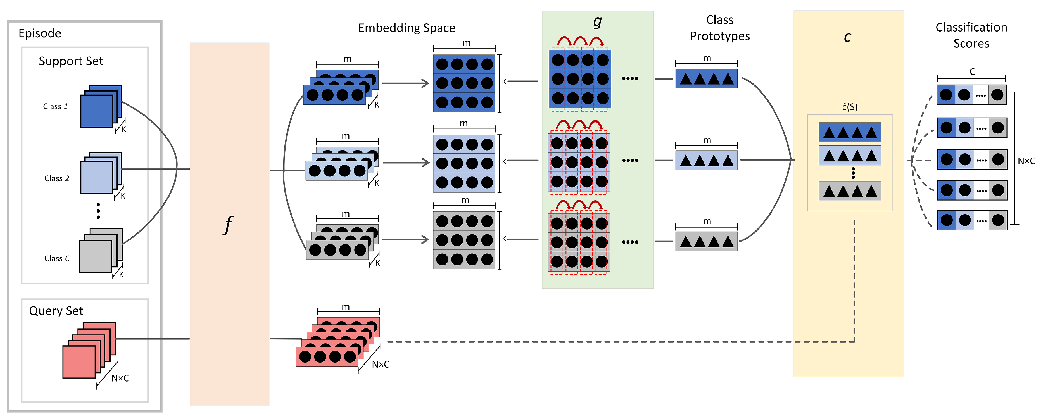
We divide the ConvProtoNet into three parts: an embedding module to project samples to feature space f, a convolutional induction module to generate class prototypes g, and a SoftMax classifier generator using modified cosine similarity function c as shown in Figure 3.

3.4.1. Embedding Module

This module mainly uses CNN as the basic element to extract features in malware images and embed malware samples to feature space. Mostly, this part is fixed in other models using four convolution layers along with pooling, batch normalization and activation in each layer. In order to avoid overfitting, this part is generally designed as a simple structure with as few parameters as possible. Although some advanced structures like VGG and ResNet are reported to be powerful [45], we did not observe significant enhancement from them in practice and this motivates us to improve the embedding structure.
We follow the four-convolution convention (Conv-4) to build embedding module but make some modifications upon it. We gradually increase the number of channels to take place of the fix number of channels (e.g., 64) to get more high-level features and adopt channel pooling after Conv-4 structure, which is a variant of Global Average Pooling (GAP) derived from [46] to prevent overfitting. Concretely, we only take the maximum value in each feature map to form the feature vector after Conv-4, which is equal to do adaptive max-pooling on feature maps where the size of kernel is set equal to feature map. It enables the model to process different sizes of malware images as long as the texture features in images are kept. The resulted feature vectors are therefore in fixed length equal to the final number of feature map m. For a malware image x, let Conv-4 structure be C o n v outputting m feature maps, the embedding e x can be obtained as:
e x = f ( x ) = [ max ( C o n v ( x ) 1 ) , . . . , max ( C o n v ( x ) m ) ]
where e x R 1 × m .
Channel pooling can cooperate with random cropping to enhance the generalization ability of model. To be specific, we use random cropping in training stage for data augmentation whereas feeding uncropped images to the trained model in testing stage to maintain data integrity and provide more discriminative features. Channel pooling can slightly increase testing accuracy by about 1% in our experiments.

3.4.2. Convolutional Prototype Induction

How to obtain class prototypes lies on heart of our approach because we do classification based on the prototypes rather than the samples in class. We expect that prototypes can be representative for the class which indicates the distribution of prototypes should be as consistent as possible with the distribution of source data. To capture this complex dependency, we use stacked convolutional layers in place of the simple arithmetic operation like mean of support set in [15] to complete the reduction. Embedded support set is reshaped to a data matrix in K × m and input to this module indentified by g. Concretely, let e i , j S denotes the j-th embedding of i-th class, the i-th class prototype x ^ i can be obtained as:
x ^ i = g ( [ e i , 1 S ; e i , 2 S ; . . . ; e i , K S ] ) ,
where x ^ i R 1 × m .
The structure of the induction module is inspired by the feature attention module of Hybrid Attention-Based Prototypical Network (HABPN) in [15], but differently we treat the output as prototypes instead of weight vector. Convolutional layers can often extract deep spatial and texture features, thus the complex implicit data distribution can be learned from the sample matrix. Additionally, we remove the last ReLU in induction module to allow both positive and negative values in class prototype vector. Removal of the last ReLU was mentioned in [10] to enrich the representation of feature vector whereas we give up the same modification to embedding module in order to keep the expressing ability of the non-linear transformation. Compared with HABPN, ConvProtoNet do not suffer from gradient vanishing problem and this will be discussed in Section 5.2.1.

3.4.3. Modified Cosine Similarity SoftMax Classifier Generator

After having class prototypes, they are incorporated with the classifier generator c to produce the task classifier c ^ ( S ) . Queried samples are embedded and input to the task classifier c ^ ( S ) where distances between them class prototypes and queried samples will be computed by distance function. Then the distances are input to SoftMax and output predicted results as probabilities. It is not suitable to directly use common L2 distance to measure the similarities between embeddings from embedding module and class prototypes from induction module due to different data magnitudes of different generators, mentioned in [10]. Cosine similarity is an ideal distance function to deal with magnitude problem because it only measures direction of vectors, which inherently normalizes vectors. Let s k , i be the similarity computed between an embedded queried sample e k Q of input x k Q and i-th class prototype x i ^ , the probability that the queried sample belongs to i-th class c i is:
P ( y k Q = c i | x k Q ) = exp ( s k , i ) j = 1 C exp ( s k , j ) ,
where s k , i is computed as:
s k , i = e k Q · x ^ i | e k Q | | x ^ i | .
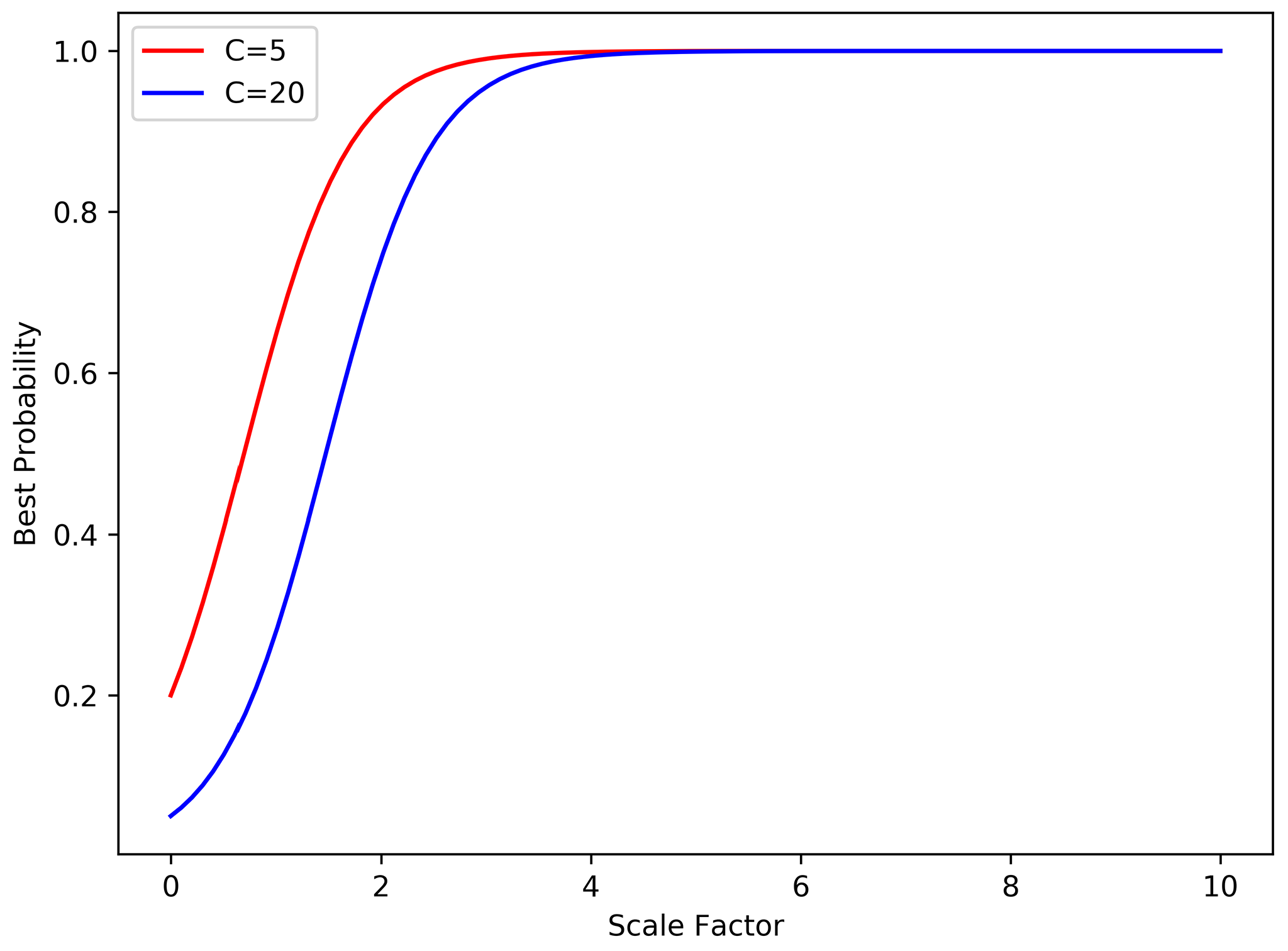
However, pure cosine similarity can result in inadequate prediction when applied into SoftMax classifier. The value of cosine similarity ranges from −1 to 1 where −1 means “not similar at all” and 1 means “most similar”. This indicates the highest probability can softmax classifier using cosine similarity produce is only e / ( e + ( N 1 ) e 1 ) , far from the ground truth probability 1. As the number of class C increases, it will drop rapidly. To address this problem, we add a scale factor α to all computed similarities as in [10,11] before applying similarities to softmax clssifier. Thus, the predicting probability changes to:
P ( y k Q = c i | x k Q ) = exp ( α · s k , i ) j = 1 C exp ( α · s k , j ) .
As shown in Figure 4, the best predicted probability can be very close to 1 when the scale factor is about 4 for C = 5 and C = 20 . Since it is unneccessary to make this scale factor changable, which is reported in [11], we fix α to 10.
The output of softmax classifier is a classification score vector with length of C in which each dimension refers the probability that queried sample belongs to the corrresponding class. It is widely acknowledged that cross entropy is a proper choice of loss function for classification problem using softmax classifier, so we use cross entropy loss for backpropagation:
L k = log ( P ( y k Q | x k Q ) ) .
For an episode, there are N × C samples in Q, so the total loss is the sum of negative log probabilities:
L = k = 1 N × C log ( P ( y k Q | x k Q ) ) .

4. Experimental Evaluation

4.1. Datasets and Preprocessing

4.1.1. Large PE Malware Dataset

This malware corpus is from [47] which is significantly large containing more than 222,700 Windows PE malware of over 500 different classes such as Trojan, Virus, Worm, Backdoor and so on. The samples are mainly downloaded from VirusTotal [48] and class tags are mostly manually labeled. Due to labeling errors, this dataset can be noisy. To filter the noise, we use an unsupervised learning method called DBSCAN [49] to detect the noisy ones among the samples tagged with the same class label and only take out samples in the same cluster to form the class. We think that wrongly tagged samples can be viewed as noise which can be separated from correctly tagged samples by DBSCAN in some extent and we further adopt the method extracting PE meta-data in [26] to get shallow representation of malware samples which will be input to DBSCAN. The minimum points in a cluster is set to 20 forcing each cluster to satisfy the scale requirement and we randomly take 20 samples out of a random cluster for each class to form a filtered dataset referred as “filtered LargePE”. There are 208 classes in filtered LargePE and we take 100 classes out of them as meta-training set, 58 classes as meta-validating set, 50 classes as meta-testing set.
Without doubt, this kind of preprocessing will make this dataset easier to fit, but also suffice to distinguish the performance of various models in malware few-shot classification. The unfiltered dataset referred as “unfiltered LargePE” is also used to test the robustness of models in a noisy scenario and there are 300 classes in meta-training set, 57 classes in meta-validating set and 50 classes in meta-testing set in unfiltered LargePE.

4.1.2. VirusShare Malware Dataset

This dataset is downloaded from VirusShare [50], an open malware sharing website, and samples in this dataset have no class labels. We use VirusTotal [48] to scan and make reports for malware in them to obtain anti-virus(AV) labels provided by third-party companies. Due to different naming schemes of AV companies, we use AVClass [51] to obtain a single canonical label for each malware file and this results in 60000 samples of about 150 classes. After labeling, we take 20 samples from each class to form the dataset referred as “VirusShare”. The meta-training set, meta-validating set and mete-testing set have 179, 50 and 50 classes respectively. No filtering is used making this dataset closer to application scenarios in real world.

4.1.3. Drebin Dataset

Drebin is an Android malware dataset of 5560 samples from 179 malware families released by MobileSandbox project [52,53]. We use this dataset in the same manner as other datasets to verify that our approach is general enough to work on datasets from different platforms. This dataset is highly class-imbalanced where some classes contain only several samples. After grouping samples by class label, only 54 classes have at least 10 samples and these classes are split to meta-training set, meta-validating set and meta-testing set having 34, 10 and 10 classes respectively. If We require more samples in each class, the number of resulted classes is too few to run meta-learning and the performance will be limited by lacking enough classes in meta-training set. For this reason, it is impossible to do 10-shot and 20-way experiments. Instead, we do 10-way experiments to replace 20-way experiments thus only 5-shot 5-way and 5-way 10-way experiments are carried out for Drebin dataset particularly.

4.2. Experiment Setup

We carry out two types of experiment to prove the feasibility of our approach to address few-shot malware classification: (1) meta-training and meta-testing on a consistent dataset; (2) meta-testing across different datasets without retraining. Each dataset is split into three parts: meta-training set, meta-validating set, and meta-testing set. Meta-validating set is used to monitor the generalization ability of the model to store the model with best validating accuracy. This is the application of early stop technique which is a common and effective trick to prevent from overfitting. We do meta-validating for 100 epochs every 100 training episodes in most experiments. We consider the setting where K = [ 5 , 10 ] and C = [ 5 , 20 ] to follow the convention in most few-shot experiments where 4 kinds of combination are resulted. We set N = 15 and N = 10 when K = 5 and K = 10 respectively.
Malware images are converted to the size of 256 × 256 without exception and 224 × 224 random cropping is taken on images during training to reduce memory consumption whereas no cropping is taken during testing stage as described. We also normalize the images when they are read into memory based on the mean and standard deviation computed on meta-training set. Other augmentation trick like random rotation is utilized as well, according to the setup in [8]. For all deep learning models, Adam optimizer is used with 10 3 as initial learning rate and 10 4 as weight decay in all cases. The learning rate will be divided by 10 every 15,000 training episodes. Models are trained for 5 × 10 4 episodes unless clear explanation is given. No fine-tuning is ever used in all experiments.

4.3. Baseline Models

Six previously proposed few-shot models are tested as baselines: Prototype Network (ProtoNet) [9], Relation Network (RelationNet) [8], Hybrid Attention-Based Prototypical Network (HABPN) [15], Induction Network (InductionNet) [14], SNAIL [38], and Meta-SGD [39]. All of these few-shot models mentioned above use the same embedding architecture described in [8] to project samples. In particular, we replace the ReLU activation function in feature attention module of HABPN with Leaky ReLU to address gradient vanishing problem encountered in experiments.
To make more comparisons, we consider three classic machine learning methods as baselines: kNN using Gist descriptors [16,54], kNN using byte n-gram frequency [17], and kNN based on image pixels. We mainly use kNN as classifier for its non-parametric nature to avoid severe overfitting. Gist and n-gram work on original PE files whereas pixel kNN uses malware images.

4.4. Validation across Different Datasets

We think it not surprising if our model trained on the meta-training set of a single malware dataset can also work on meta-testing set of another dataset because both two meta-testing sets contain classes that model have never seen during training and general knowledge is learned in the train episode iterations. To prove that our model really learns transferable knowledge, we design the validation experiment across datasets where meta-training set and meta-testing set are from different datasets. All datasets mentioned above are involved in cross validating experiments.
Here, an additional dataset, Microsoft Malware Classification Challenge Dataset (referred as Microsoft dataset in the later) released in 2015 on Kaggle [55], is taken into our consideration. This dataset contains 10868 samples from 9 families and it is hard to train a model from scratch with these few classes. Instead, we use it as a meta-testing set to test the generalization ability of our model.

4.5. Implement Details

For all the deep learning models, we use 3 × 3 kernel and max pooling stride is always 2. The number of channels in Conv-4 of ConvProtoNet increases from 1 to 32, 64, 128, and 256 that results embeddings with the length of 256 after channel pooling whereas the number of channels in other embedding modules of few-shot models is fixed at 64 as in [8]. The convolution induction module has three stacked layers following the implementation in [15] as shown in Figure 5. For RelationNet, ProtoNet, HABPN, InductionNet, SNAIL, and Meta-SGD, we implement these models without modification except keeping their embedding module to be identical Conv-4 structure.
For machine learning baselines, we use k-Nearest-Neighbor(kNN) classifier with k = 3 to avoid overfitting because kNN is an instance-based classifier rather than a parametric model requiring large number of data. We follow the approach in [17] to extract 3-gram substrings from byte sequence and take the most frequent 65,535 substrings of 3-gram as malware instance feature. PE meta-data is extracted in the same way as [26], but many samples have corrupted PE header causing failure of extracting and test results are kind of unfaithful, especially for VirusShare Dataset. Gist descriptor uses orientations of 0, π / 4 , π / 2 , and π and scales of 3, 5, 7, and 9 to build a bank of Gabor filters after a malware image is split to 8 × 8 = 64 patches. Each patch will be filtered by the built Gabor filter bank and mean of each filter’s output will be appended to the feature vector of the malware image.

4.6. Experiment Results

In almost all settings, ConvProtoNet outperforms all the baselines models with a large margin and a considerable accuracy is achieved even for noisy dataset when only a few samples in each are provided, as shown in Table 1, Table 2, Table 3 and Table 4. Suffering from convergence problem, the results of SNAIL in all 20-way settings are not reported. Among the baseline few-shot models, ProtoNet has the closest performance to ConvProtoNet, but its accuracy still falls behind by about 5% on average whereas other models have the accuracy gap over 10% on average. Experiment results on Drebin dataset show that our approach is platform-independent for malware and the minimum performance can be ensured even few classes are provided. ConvProtoNet model trained in meta-learning scheme can perform at a close level to the model trained on other datasets without retraining or fine-tuning. This indicates that our model has strong generalization ability and it can classify malware from different sources after it is trained on only one dataset once for all. The only drawback is that performance degrades with more classes to be classified and the gap is over 10% when increase from 5 classes to 20 classes. Although PE meta-data using kNN often gets high accuracy on many datasets, it will fail to work as long as the PE header of malware is corrupted deliberately or accidentally. Especially for the VirusShare dataset, it is observed that more than 15 classes have invalid PE file header causing extraction failure and the results are not entirely credible despite higher accuracy achieved by PE meta-data using kNN. It means the the approach of PE meta-data with kNN has flaw itself and it can not work on the malware datasets from different platforms like Android which limits its application. On the contrary, ConvProtoNet is platform-independent for malware and robust enough to resist to corrupted data.
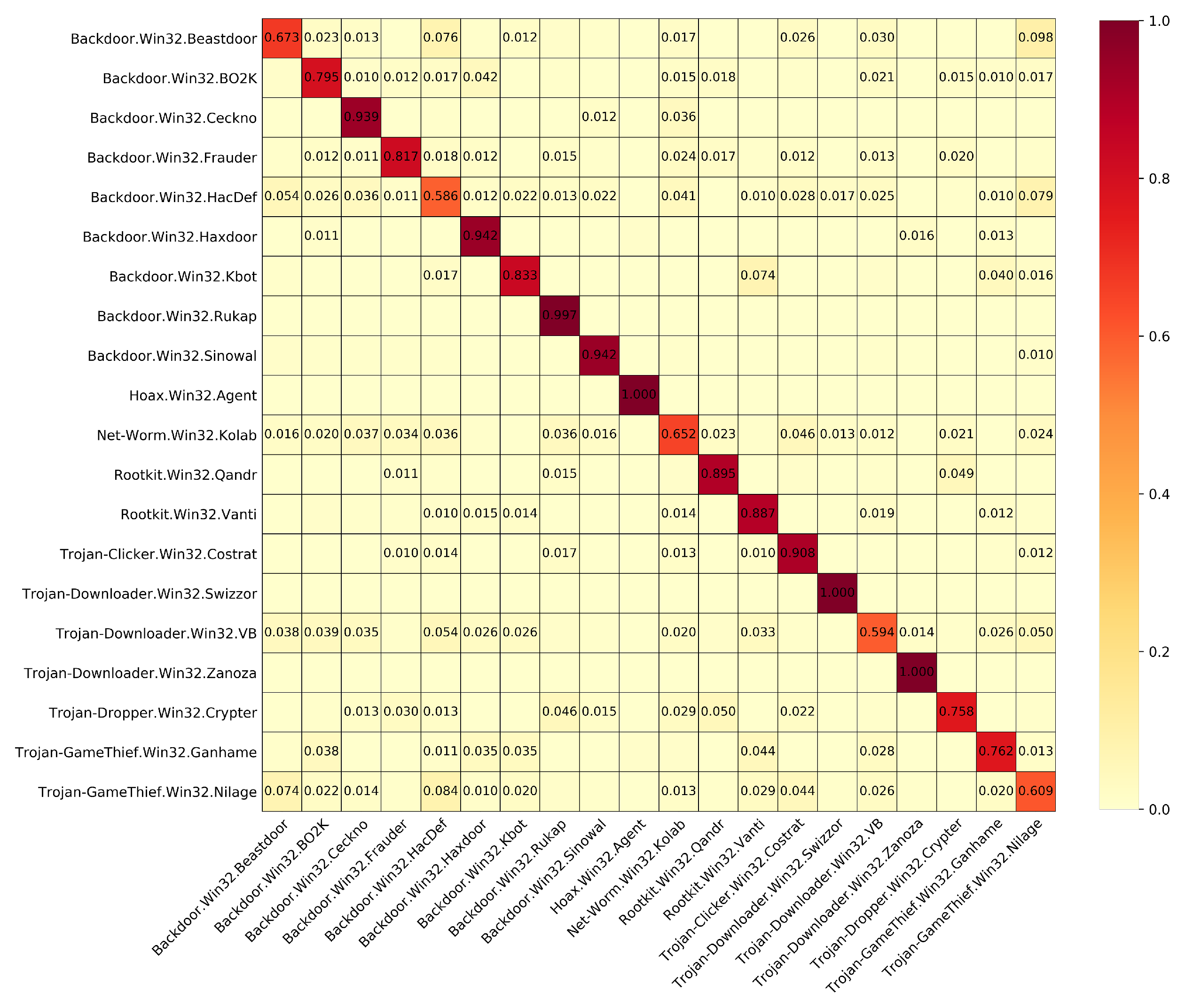
To precisely present the results ConvProtoNet achieved, we use five assessment measures: accuracy, precision, recall, F1 score and receiver operating characteristic area under curve (ROC-AUC), which is shown in Table 5. This indicates that while achiving high accuracy, ConvProtoNet keeps good balance of precision and recall. We also plot the confusion matrix of first 20 classes for 5-shot 5-way problem on LargePE dataset after 5000 testing epochs, which is shown in Figure 6. Most plotted classes can be properly handled by ConvProtoNet achieving high accuracy whereas only a few classes pull down the average accuracy.

5. Discussion and Analysis

5.1. Effectiveness of Malware Image

Malware images often tend to have special visual textures for reusing core code, repeatedly executing a same code block or carrying malicious data. Although there were a number of researches that used malware images as model input for malware analysis and proved to work well, directly converting the whole code to an image where malicious code get mixed up with the regular code seems to be rough intuitively. However, CNN structure, which is a powerful image feature extractor, is used in this research to embed the malware images and it obtains discriminative class features of malware while eliminates these irrelevant features. To prove it, we visualize the gradient backpropagated from cosine similarity in the embedding space to the original input image, as shown in Figure 7.
From the visualization, we can see that the visual texture areas which are often related to the malware characteristics have higher response sensitivity to the cosine similarity than these unstructured areas. This indicates that even when small changes occur in these texture areas, they will have significant influence on the final result whereas these plain areas will not. Also it proves that ConvProtoNet can automatically extract discriminative features from the mixed image representation and complete the classification task while ignore these useless features. Besides, malware image has many advantages over traditional malware features: Conversion from malware to image requires no expert knowledge; Images can be easily handled by modern CNN structures; Images can be visualized for interpretability; Conversion process is fast etc.

5.2. Why ConvProtoNet Works: Some Comparisons

To explain why ConvProtoNet can outperform other few-shot baselines, we carefully analyze the differences between existing few-shot models and ConvProtoNet to show the effect of some advanced designs in ConvProtoNet. Some flaws in existing few-shot are motivations for us to propose ConvProtoNet. In short, ConvProtoNet solve the problems of gradient vanishing, shallow prototype induction, poor representation, and distribution mismatching.

5.2.1. With Hybrid Attention-Based Prototypical Network

Hybrid Attention-Based Prototypical Network [15] (HABPN) is one of the few-shot baselines in experiments and accuracy of HABPN is mostly 10% lower than that of ConvProtoNet. In HABPN’s architecture, feature attention receives the embedded support set S and generates a score vector z to weight the dimensions in L2 distances between class prototypes and embedded query samples. However, the last ReLU in feature attention module makes all negative values in score vector zero which attempts to produce a sparse score vector. When backpropagating through queried loss L , the gradient of parameter ϕ e in embedding module will be also sparse for having a factor of a sparse weight vector. In specific, let f ϕ e be the embedding function, x ^ be the class prototype of a class, e i Q be the embedding of a query input x i Q , d be the distance between the class and the queried input, it goes:
d = z T ( e i Q x ^ ) 2 ,
e i Q = f ϕ e ( x i Q ) .
The gradient of parameter ϕ can be calculated using (9), (10) as following:
L ϕ e = L d · d ϕ e = 2 · z T · ( e i Q x ^ ) ( f ϕ e ϕ e x ^ ϕ e ) · L d .
From (11), it is obvious that the sparsity of z can simultaneously lead to the sparsity of gradient of ϕ e and parameters will remain unchanged even after an episode due to vanishing gradient. This negative effect will continue to grow like a snowball making learning process stop eventually. ConvProtoNet regards the output of convolution over support set as the class prototypes instead of feature attention to prevent from gradient vanishing.
Meanwhile, generation of class prototype in HABPN uses instance attention from instance attention module to suppress noise in samples. Let W I denote the instance attention, e S denote the embedded support set S, the class prototype can be obtained as:
x ^ = W I · e S .
Although it can reduce the effect of noise by decreasing the attention of noisy instance, in essence it performs linear combination over support set, and this can generate shallow prototype sometimes. Instead, ConvProtoNet uses stacked convolution layers to generate prototype which is capable to output deep class prototype through non-linear transformation.

5.2.2. With Prototype Network

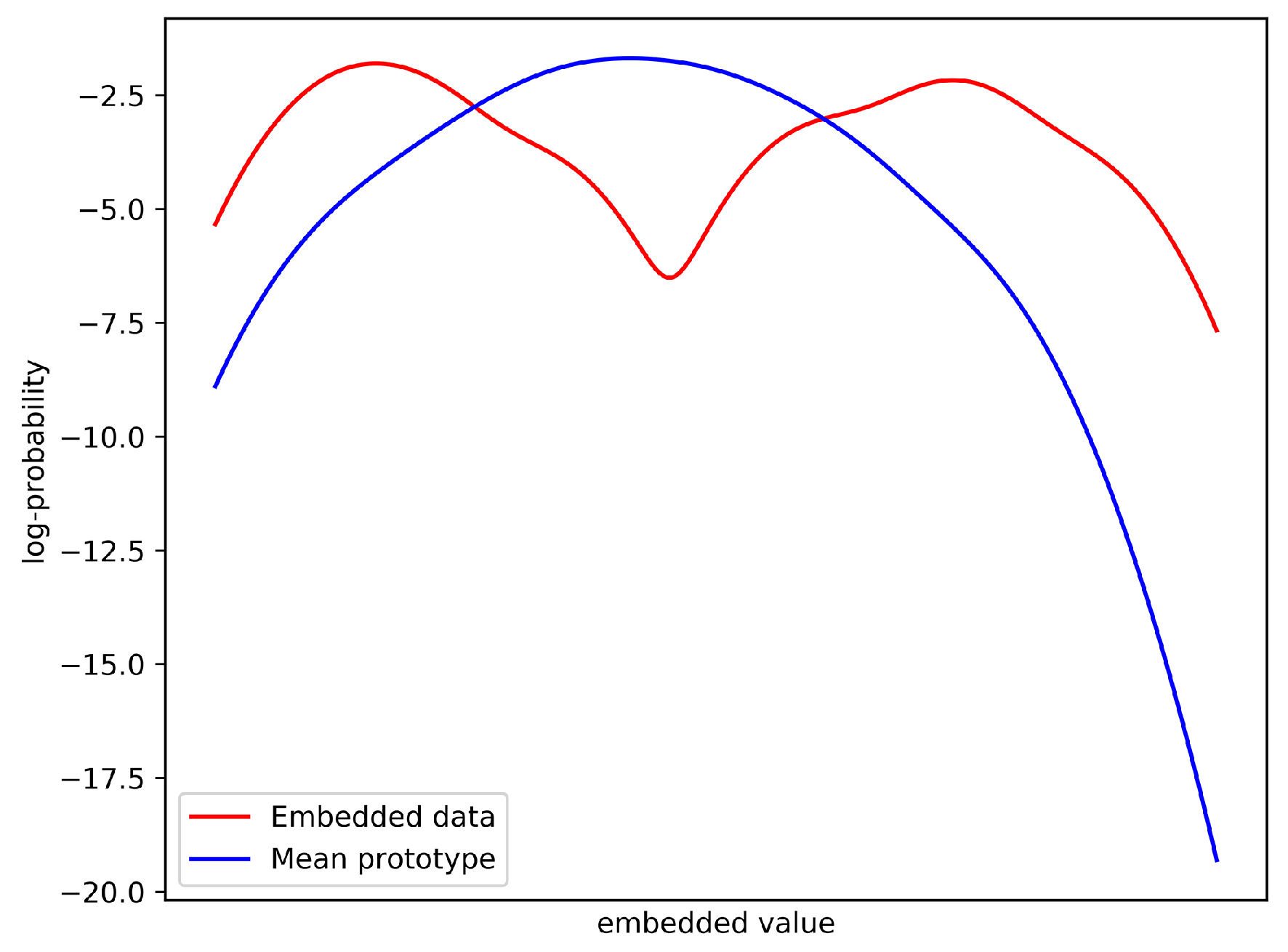
Prototypical Network (ProtoNet) [9] is one of the classic few-shot models which makes some assumptions that mean of embedded support set can represent the class distribution during meta-testing. However, this assumption only holds when each class has a unimodal distribution in the embedding space according to [11]. On the contrary, embedded data in the same class often satisfies multimodal distribution and mean of embedded support set will become an improper prototype in this case, as shown in Figure 8.
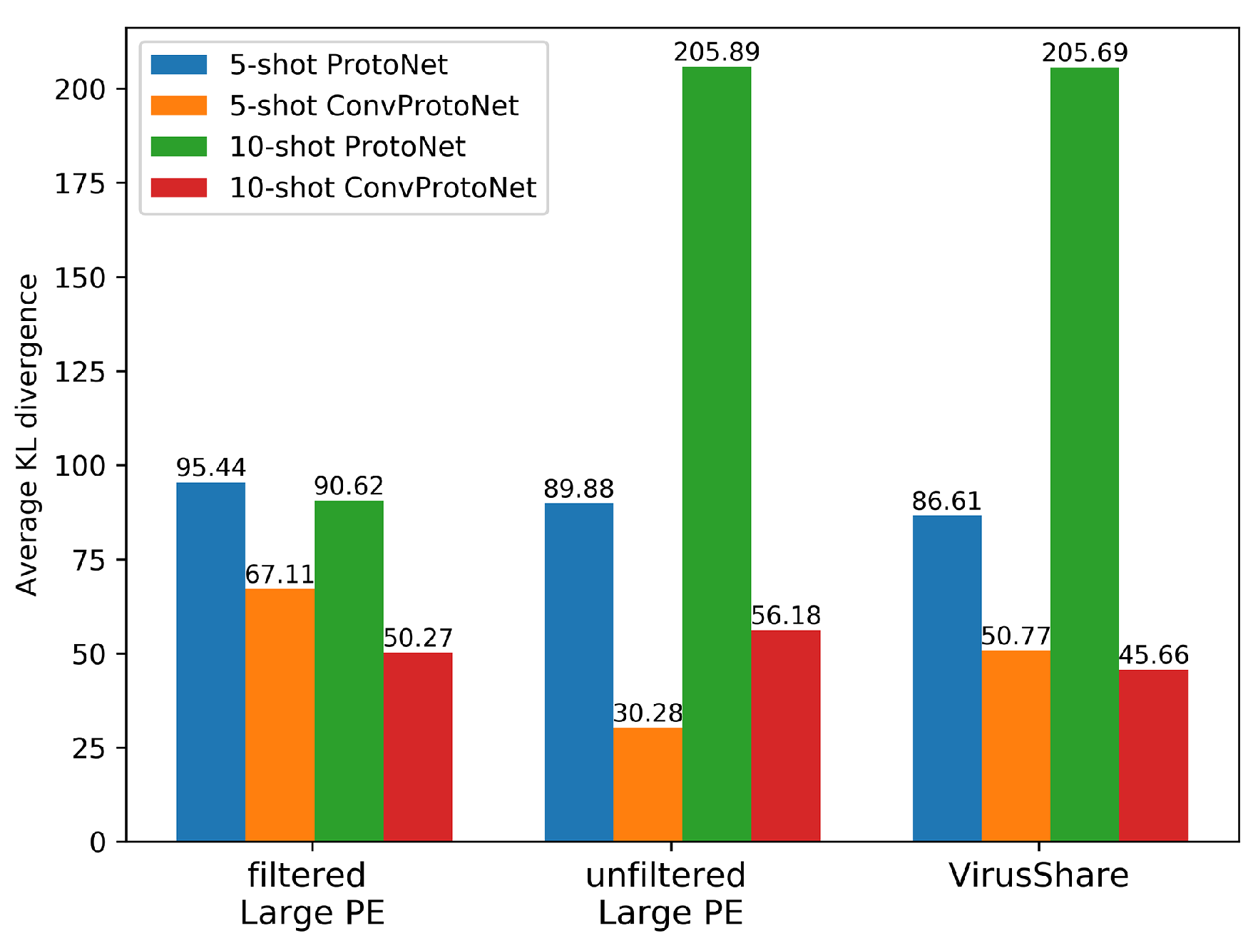
ConvProtoNet is designed to alleviate the negative effect of multimodal distribution. To demonstrate ConvProtoNet can produce more representative class prototypes than ProtoNet, we project the samples in the same class to embedding space and compute prototypes with ProtoNet and ConvProtoNet respectively. Distributions of prototypes from two models are estimated by gaussian kernel density estimation (KDE) where embedded data distribution is estimated in the same way. Finally, the fitting degree of prototype is measured by KL divergence (also called relative entropy) and results in 9 show that prototypes produced by ConvProtoNet have much lower KL divergence to the real data distribution than these produced by ProtoNet. This indicates ConvProtoNet can better handle the data satisfying multimodal distribution. Besides, Figure 9 shows that ConvProtoNet can properly process the noisy dataset whereas ProtoNet is heavily influenced by the noise. For ProtoNet, the difference between fitted distribution and real data distribution is even getting much larger when more samples ( K = 10 ) are provided.
Another shortcoming of ProtoNet is that the last ReLU in the embedding module truncates the negative values which shrinks the valid embedding space. As shown in Figure 10, because ReLU only allows positive values in the embeddings, the valid embedding space only occupies 1 / 2 D of the real vector space when the embedding space has D dimensions and this seriously limits the optimization of the model. Besides, maximum angle θ between two vectors can only be 90° in the shrinking embedding space which becomes an obstacle for cosine similarity.
In ConvProtoNet, we solve this problem by removing the last ReLU in induction module to allow negative values in prototypes described in Section 3.

5.2.3. With Induction Network

Induction Network [14] tries to improve prototype reduction using dynamic routing algorithm derived from Capsule Network [54] to replace the mean operation, where the class-level representation is calculated dynamically based on support set in a non-parametric manner. To be specific, first, each sample e i , j s in support set is transformed by transformation weights W s :
e ^ i , j s = W s e i , j s .
At each training episode, the connection strength b i of each sample in support set S is amended for several times and SoftMax is always used to make sure that coupling coefficients d i computed by b i sum to 1:
d i = s o f t m a x ( b i ) = exp ( b i ) j exp ( b j ) .
d i is used to weight the importance of each sample in S and new prototype is computed by performing linear combination:
c ^ i = j d i , j · e ^ i , j s .
Squashing operation is then applied to the new prototype:
c i = c ^ i 2 1 + c ^ i 2 c ^ i c ^ i .
At last, update the connection strength according to the new prototype:
b i , j = b i , j + e ^ i , j s · c i .
Repeating above operations for several iterations to get the final class prototype for i-th class. From (13)–(17), We can get the updating rule for connection strength at step t:
b i , j t + 1 = b i , j t + a · W s 2 · e i , j · k ( exp ( b i , k t ) e i , k ) p exp ( b i , p t ) .
where a = c ^ i 1 + c ^ i 2 is the squashing coefficient. One more step, we can get the following equation using (18):
b i , j t + 1 b i , j t 1 + a · W s 2 · e i , j 2 · exp ( b i , j t ) p exp ( b i , p t ) .
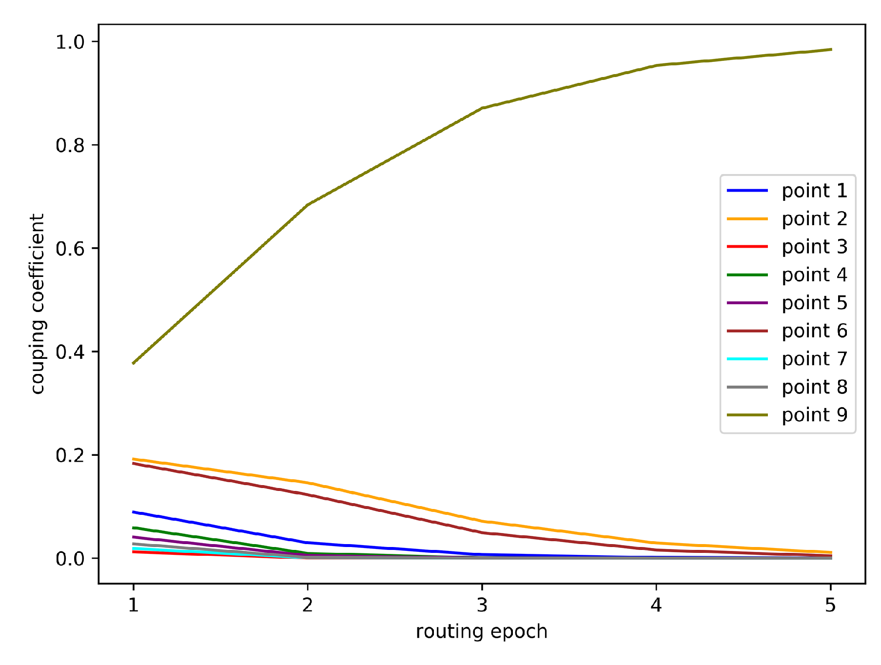
Obviously, this formula points out that bigger connection strength will grow at exponentially faster speed than other points in S. Initially, all connection strengths are set to 0 and resulted prototype is equal to mean vector of support set. After that, the generated prototype is gradually pulled to the sample point that is closest to the mean vector rapidly resulting prototypes converging at the initially closest point, as shown in Figure 11. However, in most cases, the closest point is a bad choice for class prototype. In short, InductionNet does not consider the distribution of data when computing prototype and rigid reduction yields poor performance in experiments.
For ConvProtoNet, the class prototypes are produced by stacked convolution layers where more complex mapping from samples to prototypes are performed to fit the implicit data distribution. It takes data distribution into consideration towards better reduction of prototype.

6. Future Work

We suggest some possible extensions of our work to facilitate research on few-shot malware classification. In most applications of malware classification and detection, the relatively low accuracy and precision, usually under 90%, is fatal and disastrous. However, performance is seriously constrained by scarce samples under few-shot circumstances so that more work should be done to achieve higher accuracy. First, because ConvProtoNet is a metric-based model which uses non-parametric method to classify samples, it heavily relies on good embedding of samples to make sure the accuracy of classification. Conv-4 embedding can be improved or replaced with a more powerful embedding architecture such as ResNet [34] and residual attention network [56]. Second, using multiple methods to construct hybrid malware images such as entropy and gradients in [35] is a possible way to extract more information for model training. Third, in our design, the embedding module is common and shared by all malware classes, including those unseen ones. Due to lacking explicit adaption, the accuracy may be far less than average when facing classes containing rare features. So integrating the adaptive method like MAML [37] may help. Fourth, comparing to our feature extraction method which is a kind of static analysis, dynamic analysis like API calling sequence monitoring is prone to achieve better results.
Interestingly enough, malware detection, a binary classification task that is frequently discussed in security field aiming to identify whether a program belongs to malware, can be included into malware classification task where benign files separately form a class. Thus, the scope of malware classification can cover both two tasks to solve more problems in application.

7. Conclusions

We novelly use few-shot learning approaches to address malware classification when few samples are available in this paper and propose a new model, ConvProtoNet, to improve the performance over existing few-shot models. The new model enriches the representation of embedding space, makes deep prototype induction, and prevents from gradient vanishing problem. Experiment results show that contemporary few-shot approaches are of enough ability to solve few-shot malware classification problem where considerable accuracy is achieved on several dataset and converting malware to images can retain useful information to do classification task. Besides, ConvProtoNet are also competent to work on new datasets without retraining so that continual learning may be available. More work can be carried on improving the embedding module and alleviate performance degradation when classifying more malware classes.

Author Contributions

Concept, Software, formal analysis and writing—original draft preparation, Z.T.; methodology, Z.T. and P.W.; resources, P.W.; writing—review and editing, P.W. and J.W; Supervison, Project Management, J.W. All authors have read and agreed to the published version of the manuscript.

Funding

This research received no external funding.

Acknowledgments

We greatly thank for the offer of academic access and malware scanning API from VirusTotal (https://www.virustotal.com).

Conflicts of Interest

The authors declare no conflict of interest.

References

  1. Gandotra, E.; Bansal, D.; Sofat, S. Malware analysis and classification: A survey. J. Inf. Secur. 2014, 5, 56. [Google Scholar] [CrossRef] [Green Version]
  2. Ye, Y.; Li, T.; Adjeroh, D.; Iyengar, S.S. A survey on malware detection using data mining techniques. ACM Comput. Surv. (CSUR) 2017, 50, 41. [Google Scholar] [CrossRef]
  3. Raff, E.; Barker, J.; Sylvester, J.; Brandon, R.; Catanzaro, B.; Nicholas, C.K. Malware detection by eating a whole exe. In Proceedings of the Workshops at the Thirty-Second AAAI Conference on Artificial Intelligence, New Orleans, LA, USA, 2–7 February 2018. [Google Scholar]
  4. Kolosnjaji, B.; Zarras, A.; Webster, G.; Eckert, C. Deep learning for classification of malware system call sequences. In Australasian Joint Conference on Artificial Intelligence; Springer: Cham, Switzerland, 2016; pp. 137–149. [Google Scholar]
  5. Pascanu, R.; Stokes, J.W.; Sanossian, H.; Marinescu, M.; Thomas, A. Malware classification with recurrent networks. In Proceedings of the 2015 IEEE International Conference on Acoustics, Speech and Signal Processing (ICASSP), Brisbane, Australia, 19–24 April 2015; pp. 1916–1920. [Google Scholar]
  6. Wang, Y.; Yao, Q. Few-shot learning: A survey. arXiv 2019, arXiv:1904.05046. [Google Scholar]
  7. Li, F.-F.; Fergus, R.; Perona, P. One-shot learning of object categories. IEEE Trans. Pattern Anal. Mach. Intell. 2006, 28, 594–611. [Google Scholar]
  8. Sung, F.; Yang, Y.; Zhang, L.; Xiang, T.; Torr, P.H.; Hospedales, T.M. Learning to compare: Relation network for few-shot learning. In Proceedings of the IEEE Conference on Computer Vision and Pattern Recognition, Salt Lake City, UT, USA, 18–22 June 2018; pp. 1199–1208. [Google Scholar]
  9. Snell, J.; Swersky, K.; Zemel, R. Prototypical networks for few-shot learning. In Advances in Neural Information Processing Systems; Curran Associates, Inc.: Red Hook, NY, USA, 2017; pp. 4077–4087. [Google Scholar]
  10. Gidaris, S.; Komodakis, N. Dynamic few-shot visual learning without forgetting. In Proceedings of the IEEE Conference on Computer Vision and Pattern Recognition, Salt Lake City, UT, USA, 18–22 June 2018; pp. 4367–4375. [Google Scholar]
  11. Qi, H.; Brown, M.; Lowe, D.G. Low-shot learning with imprinted weights. In Proceedings of the IEEE Conference on Computer Vision and Pattern Recognition, Salt Lake City, UT, USA, 18–22 June 2018; pp. 5822–5830. [Google Scholar]
  12. Ravi, S.; Larochelle, H. Optimization as a model for few-shot learning. In Proceedings of the International Conference on Learning Representations, Toulon, France, 24–26 April 2017. [Google Scholar]
  13. Koch, G.; Zemel, R.; Salakhutdinov, R. Siamese Neural Networks for One-Shot image Recognition. In Proceedings of the ICML Deep Learning Workshop, Lille, France, 6–11 July 2015; Volume 2. [Google Scholar]
  14. Geng, R.; Li, B.; Li, Y.; Ye, Y.; Jian, P.; Sun, J. Few-Shot Text Classification with Induction Network. arXiv 2019, arXiv:1902.10482. [Google Scholar]
  15. Gao, T.; Han, X.; Liu, Z.; Sun, M. Hybrid attention-based prototypical networks for noisy few-shot relation classification. In Proceedings of the Thirty-Second AAAI Conference on Artificial Intelligence, AAAI-19, Honolulu, HI, USA, 27 January–1 February 2019. [Google Scholar]
  16. Nataraj, L.; Karthikeyan, S.; Jacob, G.; Manjunath, B. Malware images: Visualization and automatic classification. In Proceedings of the 8th International Symposium on Visualization for Cyber Security, Pittsburgh, PA, USA, 20 July 2011; p. 4. [Google Scholar]
  17. Abou-Assaleh, T.; Cercone, N.; Keselj, V.; Sweidan, R. N-gram-based detection of new malicious code. In Proceedings of the 28th Annual International Computer Software and Applications Conference, COMPSAC 2004, Hong Kong, China, 28–30 September 2004; Volume 2, pp. 41–42. [Google Scholar]
  18. Santos, I.; Laorden, C.; Bringas, P.G. Collective classification for unknown malware detection. In Proceedings of the International Conference on Security and Cryptography, Seville, Spain, 18–21 July 2011; pp. 251–256. [Google Scholar]
  19. Anderson, B.; Storlie, C.; Lane, T. Improving malware classification: Bridging the static/dynamic gap. In Proceedings of the 5th ACM Workshop on Security and Artificial Intelligence, Raleigh, NC, USA, 19 October 2012; pp. 3–14. [Google Scholar]
  20. Santos, I.; Penya, Y.K.; Devesa, J.; Bringas, P.G. N-grams-based File Signatures for Malware Detection. ICEIS (2) 2009, 9, 317–320. [Google Scholar]
  21. Ye, Y.; Chen, L.; Wang, D.; Li, T.; Jiang, Q.; Zhao, M. SBMDS: An interpretable string based malware detection system using SVM ensemble with bagging. J. Comput. Virol. 2009, 5, 283. [Google Scholar] [CrossRef] [Green Version]
  22. Moskovitch, R.; Feher, C.; Tzachar, N.; Berger, E.; Gitelman, M.; Dolev, S.; Elovici, Y. Unknown malcode detection using opcode representation. In European Conference on Intelligence and Security Informatics; Springer: Berlin, Germany, 2008; pp. 204–215. [Google Scholar]
  23. Islam, R.; Tian, R.; Batten, L.; Versteeg, S. Classification of malware based on string and function feature selection. In Proceedings of the 2010 Second Cybercrime and Trustworthy Computing Workshop, Ballarat, Australia, 19–20 July 2010; pp. 9–17. [Google Scholar]
  24. Liu, L.; Wang, B. Malware classification using gray-scale images and ensemble learning. In Proceedings of the 2016 3rd International Conference on Systems and Informatics (ICSAI), Shanghai, China, 19–21 November 2016; pp. 1018–1022. [Google Scholar]
  25. Ucci, D.; Aniello, L.; Baldoni, R. Survey of machine learning techniques for malware analysis. Comput. Secur. 2019, 81, 123–147. [Google Scholar] [CrossRef] [Green Version]
  26. Bhodia, N.; Prajapati, P.; Di Troia, F.; Stamp, M. Transfer Learning for Image-Based Malware Classification. arXiv 2019, arXiv:1903.11551. [Google Scholar]
  27. Oliva, A.; Torralba, A. Modeling the shape of the scene: A holistic representation of the spatial envelope. Int. J. Comput. Vis. 2001, 42, 145–175. [Google Scholar] [CrossRef]
  28. Gibert, D. Convolutional Neural Networks for Malware Classification. Master’s Thesis, University Rovira i Virgili, Tarragona, Spain, 2016. [Google Scholar]
  29. Nataraj, L.; Yegneswaran, V.; Porras, P.; Zhang, J. A comparative assessment of malware classification using binary texture analysis and dynamic analysis. In Proceedings of the 4th ACM Workshop on Security and Artificial Intelligence, Chicago, IL, USA, 21 October 2011; pp. 21–30. [Google Scholar]
  30. Choi, S.; Jang, S.; Kim, Y.; Kim, J. Malware detection using malware image and deep learning. In Proceedings of the 2017 International Conference on Information and Communication Technology Convergence (ICTC), Jeju, Korea, 18–20 October 2017; pp. 1193–1195. [Google Scholar]
  31. Kim, H.J. Image-based malware classification using convolutional neural network. In Advances in Computer Science and Ubiquitous Computing; Springer: Singapore, 2017; pp. 1352–1357. [Google Scholar]
  32. Kalash, M.; Rochan, M.; Mohammed, N.; Bruce, N.D.; Wang, Y.; Iqbal, F. Malware classification with deep convolutional neural networks. In Proceedings of the 2018 9th IFIP International Conference on New Technologies, Mobility and Security (NTMS), Paris, France, 26–28 February 2018; pp. 1–5. [Google Scholar]
  33. Simonyan, K.; Zisserman, A. Very deep convolutional networks for large-scale image recognition. arXiv 2014, arXiv:1409.1556. [Google Scholar]
  34. He, K.; Zhang, X.; Ren, S.; Sun, J. Deep residual learning for image recognition. In Proceedings of the IEEE Conference on Computer Vision and Pattern Recognition, Las Vegas, NV, USA, 26 June–1 July 2016; pp. 770–778. [Google Scholar]
  35. Vu, D.L.; Nguyen, T.K.; Nguyen, T.V.; Nguyen, T.N.; Massacci, F.; Phung, P.H. A Convolutional Transformation Network for Malware Classification. arXiv 2019, arXiv:1909.07227. [Google Scholar]
  36. Vinyals, O.; Blundell, C.; Lillicrap, T.; Wierstra, D. Matching networks for one shot learning. In Advances in Neural Information Processing Systems; Curran Associates, Inc.: Red Hook, NY, USA, 2016; pp. 3630–3638. [Google Scholar]
  37. Finn, C.; Abbeel, P.; Levine, S. Model-agnostic meta-learning for fast adaptation of deep networks. In Proceedings of the 34th International Conference on Machine Learning, Sydney, Australia, 6–11 August 2017; Volume 70, pp. 1126–1135. [Google Scholar]
  38. Mishra, N.; Rohaninejad, M.; Chen, X.; Abbeel, P. A simple neural attentive meta-learner. arXiv 2017, arXiv:1707.03141. [Google Scholar]
  39. Li, Z.; Zhou, F.; Chen, F.; Li, H. Meta-sgd: Learning to learn quickly for few-shot learning. arXiv 2017, arXiv:1707.09835. [Google Scholar]
  40. Munkhdalai, T.; Yu, H. Meta networks. In Proceedings of the 34th International Conference on Machine Learning, Sydney, Australia, 6–11 August 2017; Volume 70, pp. 2554–2563. [Google Scholar]
  41. Chen, Z.; Fu, Y.; Zhang, Y.; Jiang, Y.G.; Xue, X.; Sigal, L. Semantic feature augmentation in few-shot learning. arXiv 2018, arXiv:1804.05298. [Google Scholar]
  42. Dixit, M.; Kwitt, R.; Niethammer, M.; Vasconcelos, N. Aga: Attribute-guided augmentation. In Proceedings of the IEEE Conference on Computer Vision and Pattern Recognition, Honolulu, HI, USA, 21–26 July 2017; pp. 7455–7463. [Google Scholar]
  43. Wang, Y.X.; Girshick, R.; Hebert, M.; Hariharan, B. Low-shot learning from imaginary data. In Proceedings of the IEEE Conference on Computer Vision and Pattern Recognition, Salt Lake City, UT, USA, 18–22 June 2018; pp. 7278–7286. [Google Scholar]
  44. Seok, S.; Kim, H. Visualized malware classification based-on convolutional neural network. J. Korea Inst. Inf. Secur. Cryptol. 2016, 26, 197–208. [Google Scholar] [CrossRef] [Green Version]
  45. Chen, W.Y.; Liu, Y.C.; Kira, Z.; Wang, Y.C.F.; Huang, J.B. A Closer Look at Few-shot Classification. arXiv 2019, arXiv:1904.04232. [Google Scholar]
  46. Lin, M.; Chen, Q.; Yan, S. Network in network. arXiv 2013, arXiv:1312.4400. [Google Scholar]
  47. Fang, Z.; Wang, J.; Li, B.; Wu, S.; Zhou, Y.; Huang, H. Evading anti-malware engines with deep reinforcement learning. IEEE Access 2019, 7, 48867–48879. [Google Scholar] [CrossRef]
  48. Total, V. Virustotal-Free Online Virus, Malware and Url Scanner. Available online: https://www.virustotal.com/en (accessed on 29 October 2019).
  49. Ester, M.; Kriegel, H.P.; Sander, J.; Xu, X. A density-based algorithm for discovering clusters in large spatial databases with noise. In Kdd; AAAI Press: Palo Alto, CA, USA, 1996; Volume 96, pp. 226–231. [Google Scholar]
  50. Roberts, J.M. Virus Share. 2011. Available online: https://virusshare.com (accessed on 26 October 2019).
  51. Sebastián, M.; Rivera, R.; Kotzias, P.; Caballero, J. AVclass: A Tool for Massive Malware Labeling. In International Symposium on Research in Attacks, Intrusions, and Defenses; Springer: Cham, Switzerland, 2016. [Google Scholar]
  52. Arp, D.; Spreitzenbarth, M.; Hubner, M.; Gascon, H.; Rieck, K. Drebin: Efficient and Explainable Detection of Android Malware in Your Pocket. In Proceedings of the 21th Annual Network and Distributed System Security Symposium (NDSS), San Diego, CA, USA, 23–26 February 2014. [Google Scholar]
  53. Michael, S.; Florian, E.; Thomas, S.; Felix, C.F.; Hoffmann, J. Mobilesandbox: Looking deeper into android applications. In Proceedings of the 28th International ACM Symposium on Applied Computing (SAC), Coimbra, Portugal, 18–22 March 2013. [Google Scholar]
  54. Yajamanam, S.; Selvin, V.R.S.; Di Troia, F.; Stamp, M. Deep Learning versus Gist Descriptors for Image-based Malware Classification. In Proceedings of the ICISSP, Madeira, Portugal, 22–24 January 2018; pp. 553–561. [Google Scholar]
  55. Ronen, R.; Radu, M.; Feuerstein, C.; Yom-Tov, E.; Ahmadi, M. Microsoft malware classification challenge. arXiv 2018, arXiv:1802.10135. [Google Scholar]
  56. Wang, F.; Jiang, M.; Qian, C.; Yang, S.; Li, C.; Zhang, H.; Wang, X.; Tang, X. Residual attention network for image classification. In Proceedings of the IEEE Conference on Computer Vision and Pattern Recognition, Honolulu, HI, USA, 21–26 July 2017; pp. 3156–3164. [Google Scholar]
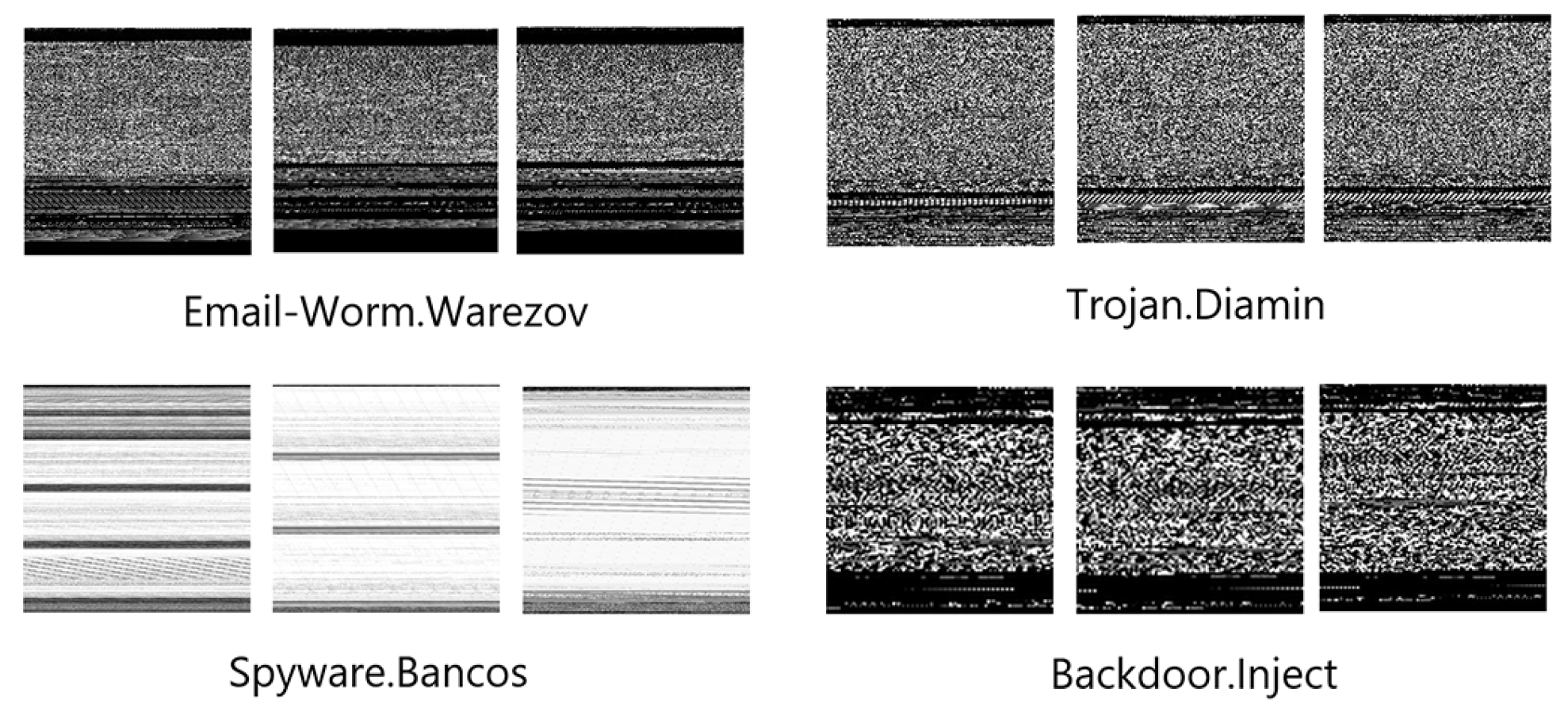
Figure 1. Some malware image examples after converting.
Applsci 10 02847 g001
Figure 2. Task structure for malware few-shot classification.
Applsci 10 02847 g002
Figure 3. Overall architecture of ConvProtoNet.
Applsci 10 02847 g003
Figure 4. Best probabilities of SoftMax classifier using cosine distance.
Applsci 10 02847 g004
Figure 5. Structure of convolutional prototype induction module g.
Applsci 10 02847 g005
Figure 6. Confusion matrix of first 20 classes in meta-testing set of LargePE dataset. Weights less than 0.01 are omitted.
Applsci 10 02847 g006
Figure 7. Gradient visualization of the malware image. Left column indicates the original malware images, and the right column indicates the corresponding gradient.
Applsci 10 02847 g007
Figure 8. An illustration of distribution mismatch using mean as prototype when data satisfy multimodal distribution.
Applsci 10 02847 g008
Figure 9. Average KL divergence between the fitted distribution generated by two models and distribution of embedded data. The distribution of prototypes from ConvProtoNet and ProtoNet are estimated by gaussian KDE on over 1000 sample points and the average KL divergence is computed for 100 epoches.
Applsci 10 02847 g009
Figure 10. An illustration of shrinking embedding space.
Applsci 10 02847 g010
Figure 11. A demo in which nine points runs dynamic routing algorithm for prototype induction.
Applsci 10 02847 g011
Table 1. Test accuracy and 95% confidence interval for malware few-shot classification on LargePE dataset. Bold items indicate the highest accuracy among all models under the same experiment setting.
ModelsFilteredUnfiltered
5-Way Acc.20-Way Acc.5-Way Acc.20-Way Acc.
5-Shot10-Shot5-Shot10-Shot5-Shot10-Shot5-Shot10-Shot
Gist + kNN [54]69.07 ± 2.8175.18 ± 2.5355.51 ± 1.6061.82 ± 1.5850.17 ± 1.6957.90 ± 1.7633.75 ± 0.8241.47 ± 0.98
N-Gram + kNN [17]46.57 ± 2.1849.37 ± 2.0436.67 ± 1.0938.30 ± 1.8036.05 ± 2.0341.64 ± 3.2425.33 ± 1.4631.22 ± 2.13
PE + kNN [26]----57.18 ± 1.1066.56 ± 1.0041.77 ± 0.8251.09 ± 0.84
pixel kNN63.60 ± 0.9467.39 ± 0.9642.49 ± 0.5845.22 ± 0.4245.11 ± 0.6447.81 ± 0.6716.87 ± 0.3119.39 ± 0.30
InductionNet [14]68.08 ± 0.3869.17 ± 0.1942.09 ± 0.0944.24 ± 0.1845.09 ± 0.3652.33 ± 0.3528.13 ± 0.1628.88 ± 0.15
SNAIL [38]73.81 ± 0.3675.13 ± 0.35--52.87 ± 0.3557.29 ± 0.34--
Meta-SGD [39]75.54 ± 0.3177.84 ± 0.3144.85 ± 0.1846.89 ± 0.1860.47 ± 0.3163.37 ± 0.3137.06 ± 0.1438.31 ± 0.16
ProtoNet [9]79.57 ± 0.2282.63 ± 0.2063.31 ± 0.1265.00 ± 0.1163.51 ± 0.1666.73 ± 0.1543.22 ± 0.0847.58 ± 0.07
RelationNet [8]74.98 ± 0.2377.28 ± 0.2353.13 ± 0.1257.48 ± 0.1361.41 ± 0.1660.05 ± 0.1738.45 ± 0.0839.50 ± 0.09
HABPN [15]80.19 ± 0.2082.24 ± 0.2156.34 ± 0.1959.44 ± 0.1858.78 ± 0.2365.62 ± 0.1540.32 ± 0.0940.67 ± 0.08
ConvProtoNet83.34 ± 0.1386.63 ± 0.1368.56 ± 0.0871.38 ± 0.0868.07 ± 0.2371.22 ± 0.1548.61 ± 0.0753.53 ± 0.08
Table 2. Test accuracy and 95% confidence interval for malware few-shot classification on VirusShare dataset. Note that PE meta-data often fails to extract features for corrupted PE header of many classes. Bold items indicate the highest accuracy among all models under the same experiment setting.
Models5-Way Acc.20-Way Acc.
5-Shot10-Shot5-Shot10-Shot
Gist + kNN [54]59.91 ± 2.8569.28 ± 2.2544.34 ± 1.3252.99 ± 1.47
N-Gram + kNN [17]54.75 ± 2.8057.08 ± 2.0047.56 ± 2.3447.88 ± 2.04
PE + kNN [26]70.58 ± 1.0378.51 ± 0.9256.58 ± 1.6864.81 ± 1.88
pixel kNN51.06 ± 1.1153.94 ± 1.2433.24 ± 0.6038.64 ± 0.63
InductionNet [14]54.10 ± 0.3756.61 ± 0.3736.33 ± 0.1843.20 ± 0.18
SNAIL [38]54.60 ± 0.3759.11 ± 0.35--
Meta-SGD [39]65.15 ± 0.3267.72 ± 0.3141.79 ± 0.1844.44 ± 0.17
ProtoNet [9]69.80 ± 0.3576.78 ± 0.2358.13 ± 0.1263.42 ± 0.11
RelationNet [8]65.42 ± 0.2267.53 ± 0.2346.12 ± 0.1149.05 ± 0.12
HABPN [15]67.70 ± 0.2370.83 ± 0.2349.78 ± 0.1154.18 ± 0.12
ConvProtoNet75.59 ± 0.2280.30 ± 0.4559.17 ± 0.2464.03 ± 0.23
Table 3. Test accuracy and 95% confidence interval for malware few-shot classification on Drebin dataset. Drebin contains Android applications thus PE meta-data experiments are not reported. Bold items indicate the highest accuracy among all models under the same experiment setting.
Models5-Shot
5-Way Acc.10-Way Acc.
Gist + kNN [54]62.06 ± 2.0050.71 ± 1.48
N-Gram + kNN [17]57.82 ± 2.0748.88 ± 2.12
PE + kNN [26]--
pixel kNN33.40 ± 0.9024.39 ± 0.61
InductionNet [14]42.87 ± 0.3231.10 ± 0.18
SNAIL [38]47.95 ± 0.3725.21 ± 0.16
Meta-SGD [39]54.01 ± 0.3437.94 ± 0.14
ProtoNet [9]66.14 ± 0.2451.05 ± 0.10
RelationNet [8]52.39 ± 0.2340.37 ± 0.10
HABPN [15]56.90 ± 0.2443.58 ± 0.09
ConvProtoNet68.58 ± 0.2257.10 ± 0.09
Table 4. Test accuracy for malware 5-shot 5-way classification of ConvProtoNet across different datasets and 95% confidence interval is attached after accuracy. Base dataset refers to the dataset that model trains on and tested dataset refers to the dataset that uses as meta-testing set and the native accuracy of each datatset is in bold.
Base DatasetsTested Dataset
LargePE
(Filtered)
LargePE
(Unfiltered)
MicrosoftVirusShareDrebin
LargePE (filtered)83.34 ± 0.1363.19 ± 0.2377.19 ± 0.1570.02 ± 0.2457.42 ± 0.24
LargePE (unfiltered)83.85 ± 0.1968.07 ± 0.2378.29 ± 0.1571.87 ± 0.2452.34 ± 0.21
VirusShare81.34 ± 0.2163.47 ± 0.2377.77 ± 0.1675.59 ± 0.2260.01 ± 0.21
Drebin74.61 ± 0.2452.91 ± 0.2473.69 ± 0.1962.21 ± 0.2568.58 ± 0.22
Table 5. Performance assessment measures for 5-shot 5-way problem.
MeasuresDatasets
Filtered
LargePE
Unfiltered
LargePE
VirusShareDrebin
Accuracy0.83340.68070.75590.6858
Precision0.83490.68930.76660.6966
Recall0.82250.67780.75450.6623
F1 Score0.81580.66840.74600.6494
AUC0.95680.89780.93490.8831