Boiling Flow Pattern Identification Using a Self-Organizing Map


Abstract
1. Introduction
2. Materials and Methods
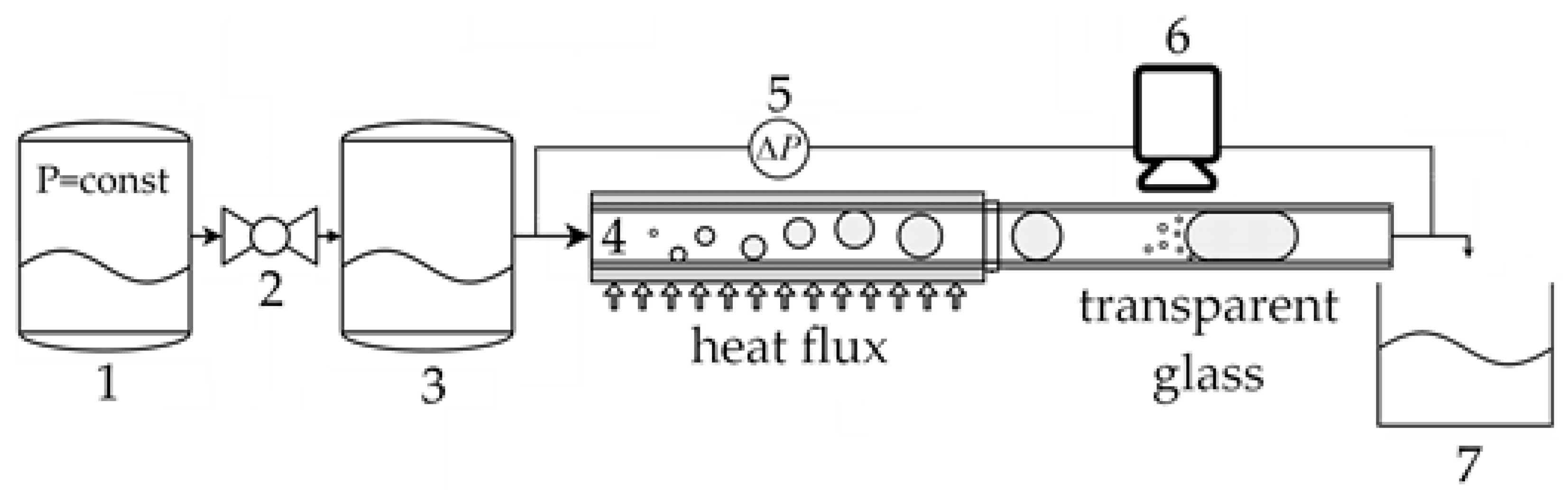
2.1. Experimental Setup
2.2. Recurrence Quantification Analysis
2.3. Self-Organizing Map
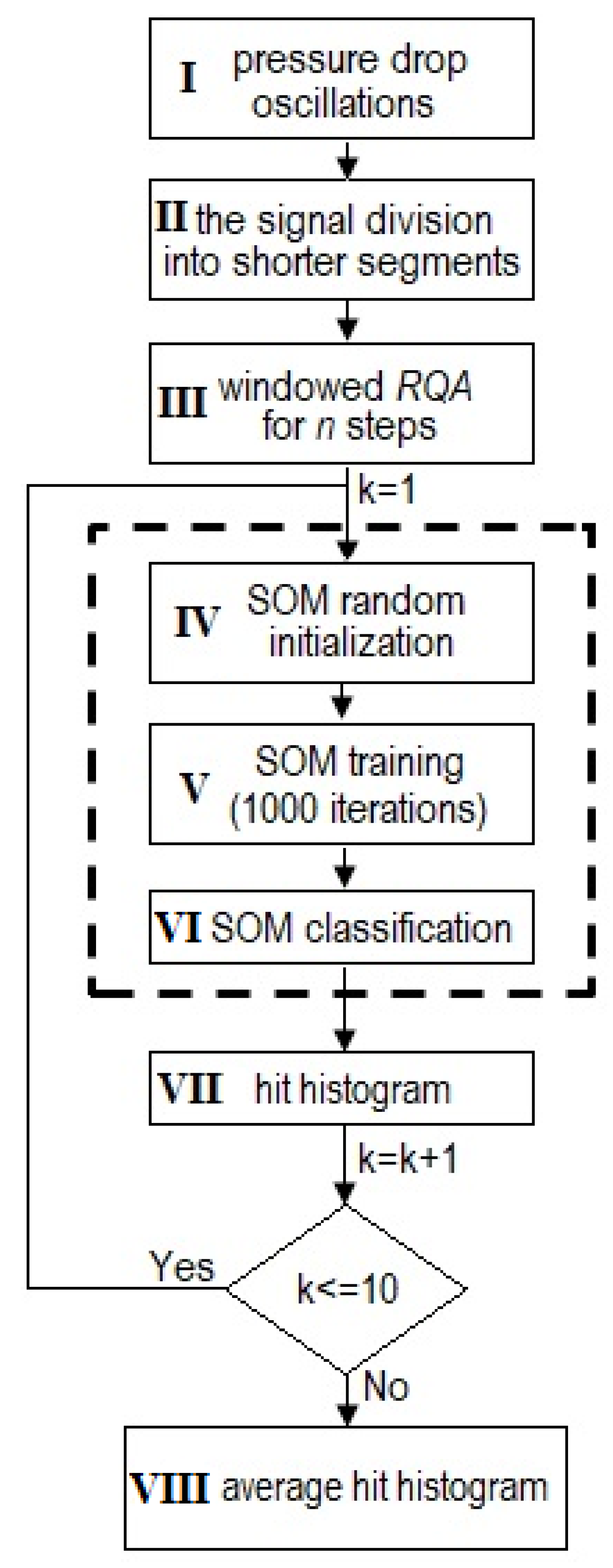
- Loading the pressure drop oscillations;
- The division of the signal (185,000 samples) into segments of 5000 samples;
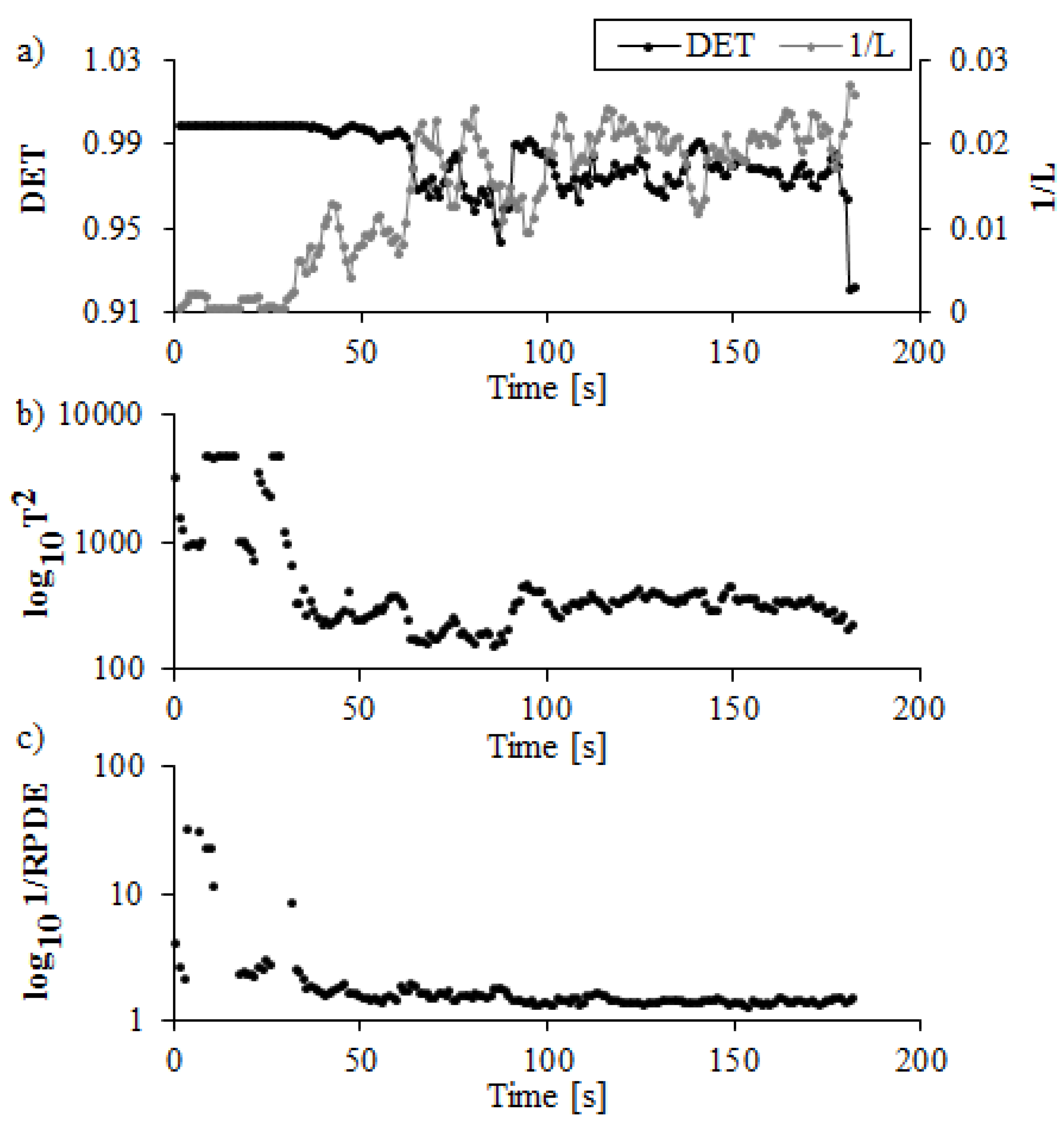
- Conducting the windowed RQA analysis for each segment. As the results of the analysis, the matrix containing the RQA coefficients is being created (DET, 1/L, T2 and 1/RPDE).
- SOM random initialization;
- SOM training using 1000 iterations;
- Comparison of each test vector with prototypes of the map (SOM classification);
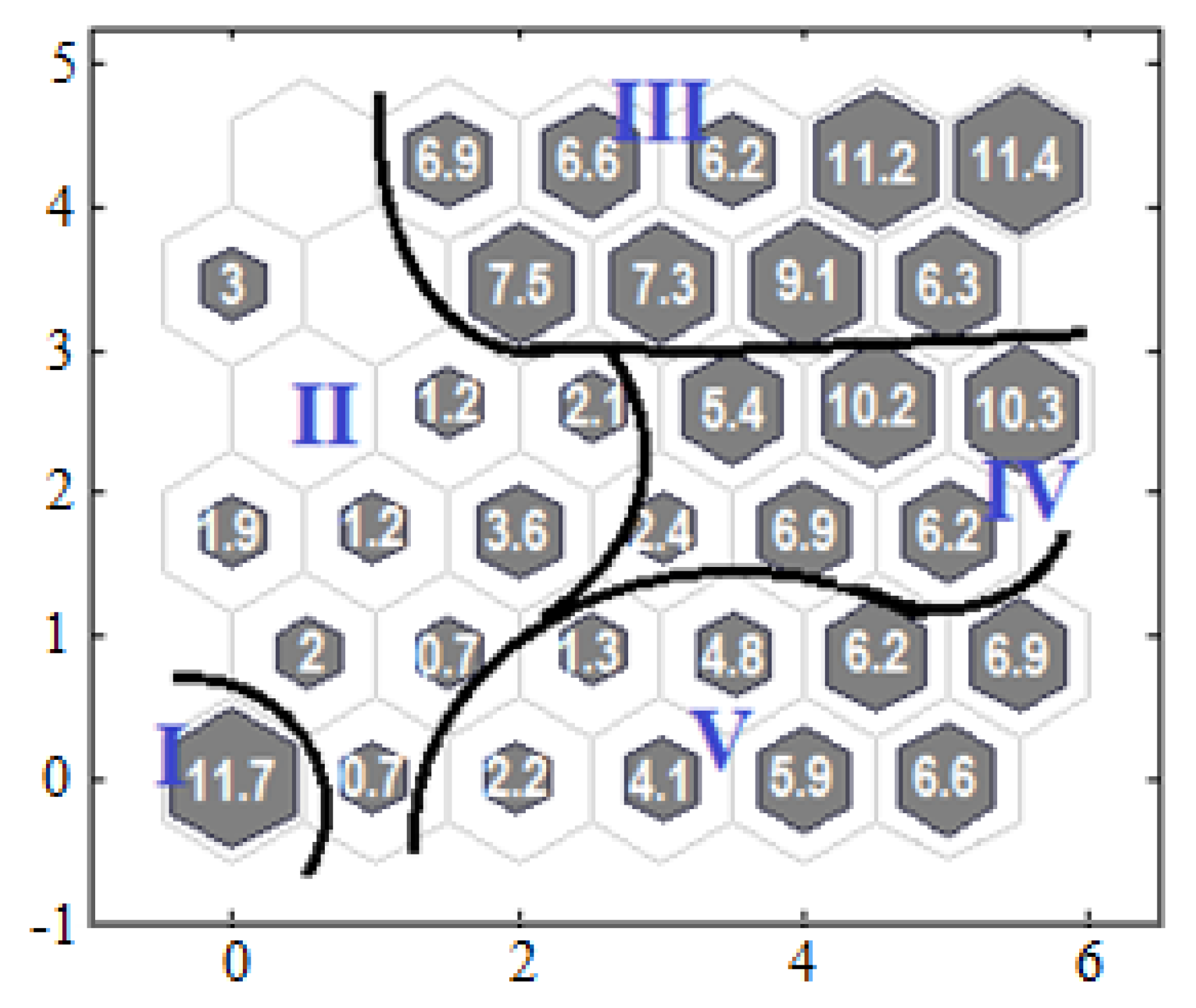
- Obtaining the results of SOM analysis—the hit histogram is created;
- After receiving 10 results of the SOM analysis, the average hit histogram is constructed.
3. Results and Discussion
4. Conclusions
Author Contributions
Funding
Conflicts of Interest
Nomenclature
| CRP | cross recurrence plot |
| DET | determinism |
| DWO | density wave oscillations |
| G | mass flux, kg/m2s |
| j | number of neurons in the network |
| k | iteration step |
| L | average length of diagonal lines (number of samples) |
| l | length of diagonal line |
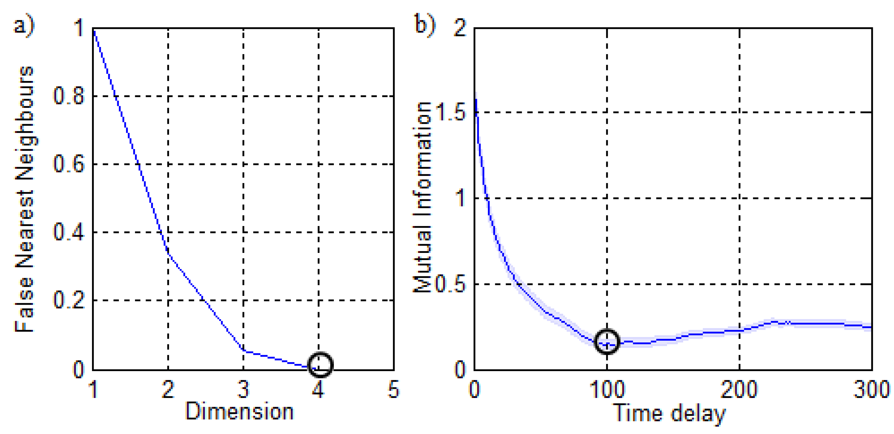
| m | embedding dimension |
| N | number of samples or length of time series |
| n | number of row in matrix |
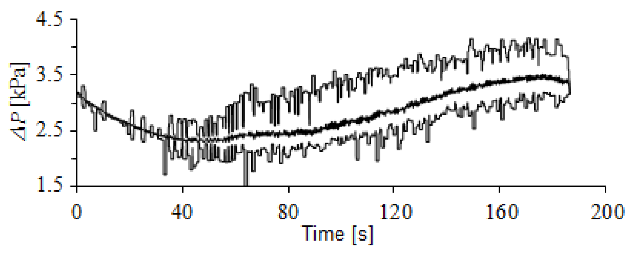
| ΔP | pressure drop Pa |
| P | heat input (W) |
| P(l) | distribution of diagonal line length |
| P(t) | recurrence period density function |
| PCA | principal component analysis |
| PDO | pressure drop oscillation |
| R | recurrence matrix |
| R | set of real numbers |
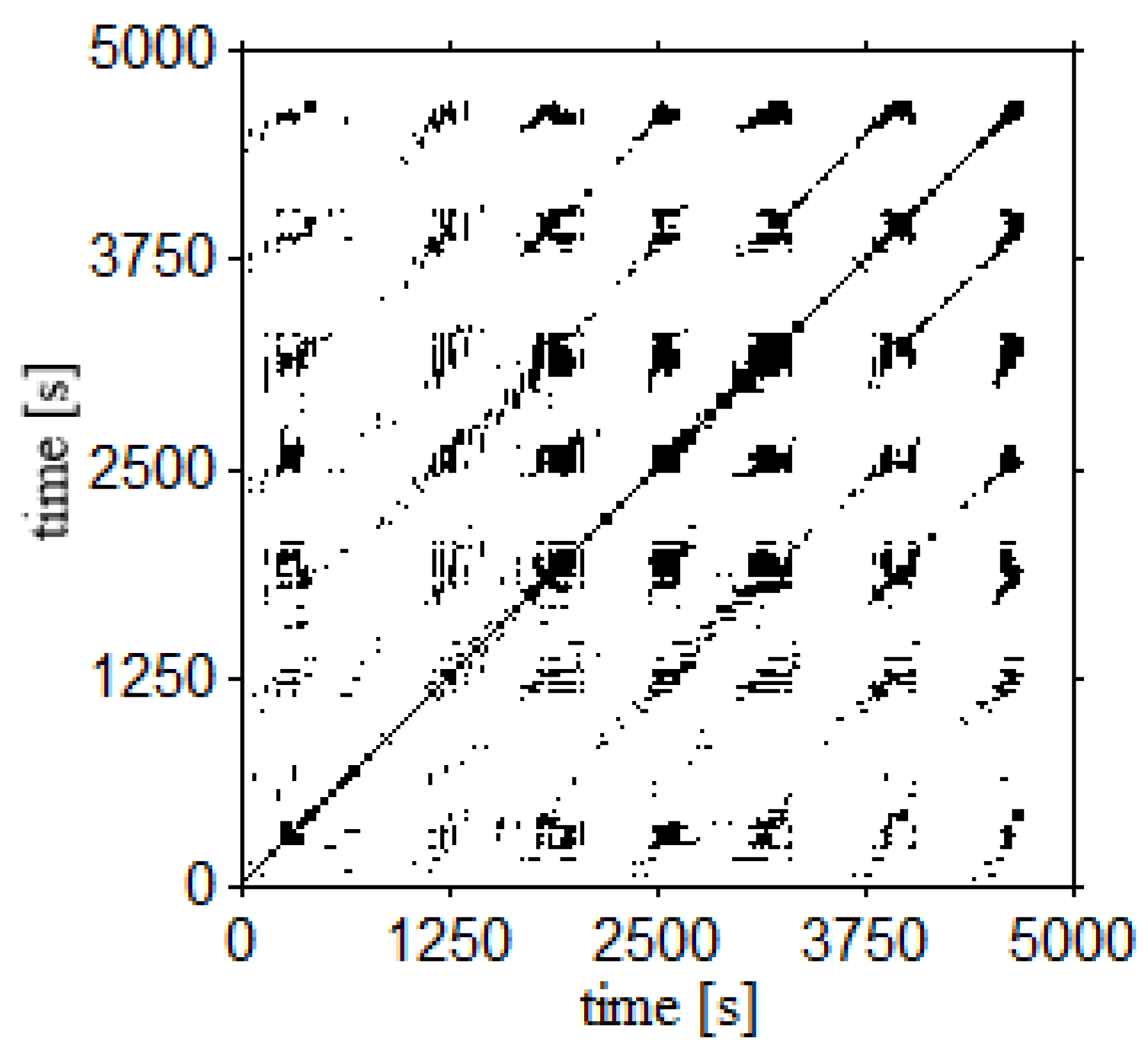
| RP | recurrence plot |
| RPDE | recurrence period density entropy |
| RQA | recurrence quantification analysis |
| SOM | self-organizing map |
| t | time (s) |
| T2 | recurrence time of 2nd type |
| W | weight vector |
| x | measured value |
| X | input matrix |
| Y | the output vector of SOM algorithm |
| Greek Symbols | |
| ε | threshold for RP computation |
| Θ | Heaviside function |
| τ | time delay (samples) |
| λ | the learning constant |
| Subscripts | |
| i, j | indices |
| m | dimensional space |
| max | maximum |
| min | minimum |
References
- Quibén, J.M.; Cheng, L.; da Silva Lima, R.J.; Thome, J.R. Flow boiling in horizontal flattened tubes: Part II—Flow boiling heat transfer results and model. Int. J. Heat Mass Transf. 2009, 52, 3645–3653. [Google Scholar] [CrossRef]
- Asadi, M.; Xie, G.; Sundén, B. A review of heat transfer and pressure drop characteristics of single and two-phase microchannels. Int. J. Heat Mass Transf. 2014, 79, 34–53. [Google Scholar] [CrossRef]
- Ruspini, L.C.; Marcel, C.P.; Clausse, A. Two-phase flow instabilities: A review. Int. J. Heat Mass Transf. 2014, 71, 521–548. [Google Scholar] [CrossRef]
- Prajapati, Y.; Bhandari, P. Flow boiling instabilityies in microchannels and their promising solutions—A review. Exp. Therm. Fluid Sci. 2017, 88, 576–593. [Google Scholar] [CrossRef]
- Sheykhi, M.R.; Afrand, M.; Toghraie, D.; Talebizadehsardari, P. Numerical simulation of critical heat flux in forced boiling of a flow in an inclined tube with different angles. J. Therm. Anal. Calorim. 2020, 139, 2859–2880. [Google Scholar] [CrossRef]
- Azadbakhti, R.; Pourfattah, F.; Ahmadi, A.; Akbari, O.A.; Toghraie, D. Eulerian–Eulerian multi-phase RPI modeling of turbulent forced convective of boiling flow inside the tube with porous medium. Int. J. Numer. Method Heat Fluid Flow 2019. ahead-of-print. [Google Scholar] [CrossRef]
- Peng, Y.; Zarringhalam, M.; Hajian, M.; Toghraie, D.; Tadi, S.J.; Afrand, M. Empowering the boiling condition of Argon flow inside a rectangular microchannel with suspending Silver nanoparticles by using of molecular dynamics simulation. J. Mol. Liq. 2019, 295, 111721. [Google Scholar] [CrossRef]
- Zong, L.X.; Xia, G.D.; Jia, Y.T.; Liu, L.; Ma, D.D.; Wang, J. Flow boiling instability characteristics in microchannels with porous-wall. Int. J. Heat Mass Transf. 2020, 146, 118863. [Google Scholar] [CrossRef]
- Xia, G.; Lv, Y.; Ma, D.; Jia, Y. Experimental investigation of the continuous two-phase instable boiling in microchannels with triangular corrugations and prediction for instable boundaries. Appl. Therm. Eng. 2019, 162, 114251. [Google Scholar] [CrossRef]
- Park, I.W.; Fernandino, M.; Dorao, C.A. On the occurrence of superimposed density wave oscillations on pressure drop oscillations and the influence of a compressible volume. AIP Adv. 2018, 8, 075022. [Google Scholar] [CrossRef]
- Park, I.W.; Ryu, J.; Fernandino, M.; Dorao, C.A. Can flow oscillations during flow boiling deteriorate the heat transfer coefficient? Appl. Phys. Lett. 2018, 113, 154102. [Google Scholar] [CrossRef]
- O’Neill, L.E.; Mudawar, I.; Hasan, M.M.; Nahra, H.K.; Balasubramaniam, R.; Mackey, J.R. Experimental investigation of frequency and amplitude of density wave oscillations in vertical upflow boiling. Int. J. Heat Mass Transf. 2018, 125, 1240–1263. [Google Scholar] [CrossRef] [PubMed]
- Mahmoud, M.M.; Karayiannis, T.G. Flow pattern transition models and correlations for flow boiling in mini-tubes. Exp. Therm. Fluid Sci. 2016, 70, 270–282. [Google Scholar] [CrossRef]
- Karayiannis, T.G.; Mahmoud, M.M. Flow boiling in microchannels: Fundamentals and applications. Appl. Therm. Eng. 2017, 115, 1372–1397. [Google Scholar] [CrossRef]
- Nandagopal, M.S.G.; Abraham, E.; Selvaraju, N. Advanced neural network prediction and system identification of liquid-liquid flow patterns in circular microchannels with varying angle of confluence. Chem. Eng. J. 2017, 309, 850–865. [Google Scholar] [CrossRef]
- Xiao, J.; Luo, X.; Feng, Z.; Zhang, J. Using artificial intelligence to improve identification of nanofluid gas–liquid two-phase flow pattern in mini-channel. AIP Adv. 2018, 8, 015123. [Google Scholar] [CrossRef]
- Mosdorf, R.; Górski, G. Detection of two-phase flow patterns using the recurrence network analysis of pressure drop fluctuations. Int. Commun. Heat Mass Transf. 2015, 64, 14–20. [Google Scholar] [CrossRef]
- Monni, G.; De Salve, M.; Panella, B. Horizontal two-phase flow pattern recognition. Exp. Therm. Fluid Sci. 2014, 59, 213–221. [Google Scholar] [CrossRef][Green Version]
- Cai, S.; Toral, H.; Qiu, J.; Archer, J.S. Neural network based objective flow regime identification in air-water two phase flow. Can. J. Chem. Eng. 1994, 72, 440–445. [Google Scholar] [CrossRef]
- Sun, B.; Chang, H.; Zhou, Y.-L. Flow Regime Recognition and Dynamic Characteristics Analysis of Air-Water Flow in Horizontal Channel under Nonlinear Oscillation Based on Multi-Scale Entropy. Entropy 2019, 21, 667. [Google Scholar] [CrossRef]
- Liu, F.; Zhang, B.; Yang, Z. Lyapunov stability and numerical analysis of excursive instability for forced two-phase boiling flow in a horizontal channel. Appl. Therm. Eng. 2019, 159, 113664. [Google Scholar] [CrossRef]
- Grzybowski, H.; Mosdorf, R. Dynamics of pressure drop oscillations during flow boiling inside minichannel. Int. Commun. Heat Mass Transf. 2018, 95, 25–32. [Google Scholar] [CrossRef]
- Marwan, N.; Carmen Romano, M.; Thiel, M.; Kurths, J. Recurrence plots for the analysis of complex systems. Phys. Rep. 2007, 438, 237–329. [Google Scholar] [CrossRef]
- Eckmann, J.-P.; Kamphorst, S.O.; Ruelle, D. Recurrence Plots of Dynamical Systems. EPL 1987, 4, 973–977. [Google Scholar] [CrossRef]
- Takens, F. Detecting strange attractors in turbulence. In Lecture Notes in Mathematics, Dynamical Systems and Turbulence; Rand, D., Young, L.S., Eds.; Springer: Berlin/Heidelberg, Germany, 1981; Volume 898, pp. 366–381. [Google Scholar]
- Roulston, M.S. Estimating the errors on measured entropy and mutual information. Phys. D 1999, 125, 285–294. [Google Scholar] [CrossRef]
- Marwan, N. Cross Recurrence Plot Toolbox for MATLAB®, Ver. 5.21 (R31c). Available online: http://tocsy.pik-potsdam.de/CRPtoolbox/ (accessed on 5 April 2020).
- Mindlin, G.M.; Gilmore, R. Topological analysis and synthesis of chaotic time series. Phys. D 1992, 58, 229–242. [Google Scholar] [CrossRef]
- Koebbe, M.; Mayer-kress, G.; Zbilut, J. Use of Recurrence Plots in the Analysis of Time-Series Data. In Nonlinear Modeling and Forecasting; Casdagli, M., Eubank, S., Eds.; Addison-Wesley: Reading, MA, USA, 1991; pp. 361–378. [Google Scholar]
- Zbilut, J.P.; Webber, C.L. Embeddings and delays as derived from quantification of recurrence plots. Phys. Lett. A 1992, 171, 199–203. [Google Scholar] [CrossRef]
- Zbilut, J.P.; Zaldivar-Comenges, J.-M.; Strozzi, F. Recurrence quantification based Lyapunov exponents for monitoring divergence in experimental data. Phys. Lett. A 2002, 297, 173–181. [Google Scholar] [CrossRef]
- Gao, J.B. Recurrence Time Statistics for Chaotic Systems and Their Applications. Phys. Rev. Lett. 1999, 83, 3178–3181. [Google Scholar] [CrossRef]
- Mukherjee, S.; Palit, S.K.; Banerjee, S.; Ariffin, M.R.K.; Rondoni, L.; Bhattacharya, D.K. Can complexity decrease in congestive heart failure? Phys. A 2015, 439, 93–102. [Google Scholar] [CrossRef]
- Nair, A.; Kiasaleh, K. Function mapped trajectory estimation for ECG sets. Biomed. Eng. Lett. 2014, 4, 277–284. [Google Scholar] [CrossRef]
- Kohonen, T. Self-organized formation of topologically correct feature maps. Biol. Cybern. 1982, 43, 59–69. [Google Scholar] [CrossRef]
- Barbosa, P.R.; Crivelaro, K.C.O.; Seleghim, P., Jr. On the application of self-organizing neural networks in gas-liquid and gas-solid flow regime identification. J. Braz. Soc. Mech. Sci. Eng. 2010, 32, 15–20. [Google Scholar] [CrossRef][Green Version]
- Abbasi Hoseini, A.; Zavareh, Z.; Lundell, F.; Anderson, H.I. Rod-like particles matching algorithm based on SOM neural network in dispersed two-phase flow measurements. Exp. Fluids 2014, 55, 1705. [Google Scholar] [CrossRef]
- de Mesquita, R.N.; Castro, L.F.; Torres, W.M.; Rocha, M.d.S.; Umbehaun, P.E.; Andrade, D.A.; Sabundjian, G.; Masotti, P.H.F. Classification of natural circulation two-phase flow image patterns based on self-organizing maps of full frame DCT coefficients. Nucl. Eng. Des. 2018, 335, 161–171. [Google Scholar] [CrossRef]
- Abell, L. Neural Networks and Applications Using Matlab: Fit Data, Classify Patterns, Cluster Data and Time Series; CreateSpace Independent Publishing Platform: North Charleston, SC, USA, 2017. [Google Scholar]


© 2020 by the authors. Licensee MDPI, Basel, Switzerland. This article is an open access article distributed under the terms and conditions of the Creative Commons Attribution (CC BY) license (http://creativecommons.org/licenses/by/4.0/).
Share and Cite
Zaborowska, I.; Grzybowski, H.; Mosdorf, R. Boiling Flow Pattern Identification Using a Self-Organizing Map. Appl. Sci. 2020, 10, 2792. https://doi.org/10.3390/app10082792
Zaborowska I, Grzybowski H, Mosdorf R. Boiling Flow Pattern Identification Using a Self-Organizing Map. Applied Sciences. 2020; 10(8):2792. https://doi.org/10.3390/app10082792
Chicago/Turabian StyleZaborowska, Iwona, Hubert Grzybowski, and Romuald Mosdorf. 2020. "Boiling Flow Pattern Identification Using a Self-Organizing Map" Applied Sciences 10, no. 8: 2792. https://doi.org/10.3390/app10082792
APA StyleZaborowska, I., Grzybowski, H., & Mosdorf, R. (2020). Boiling Flow Pattern Identification Using a Self-Organizing Map. Applied Sciences, 10(8), 2792. https://doi.org/10.3390/app10082792