Intelligent Computer-Aided Diagnostic System for Magnifying Endoscopy Images of Superficial Esophageal Squamous Cell Carcinoma


Abstract
1. Introduction
2. Related Works
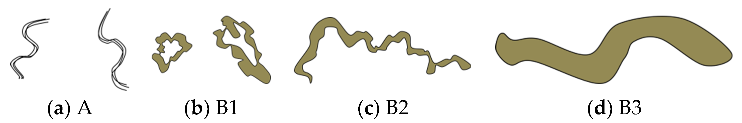
2.1. Esophageal Cancer Classification Method
2.2. Support Vector Machine Algorithm
2.3. Microvessel Thickness Measurement Algorithm Using the Least Squares Method
2.4. Extraction of Retinal Vessels and Thickness Measurement in Fundus Images
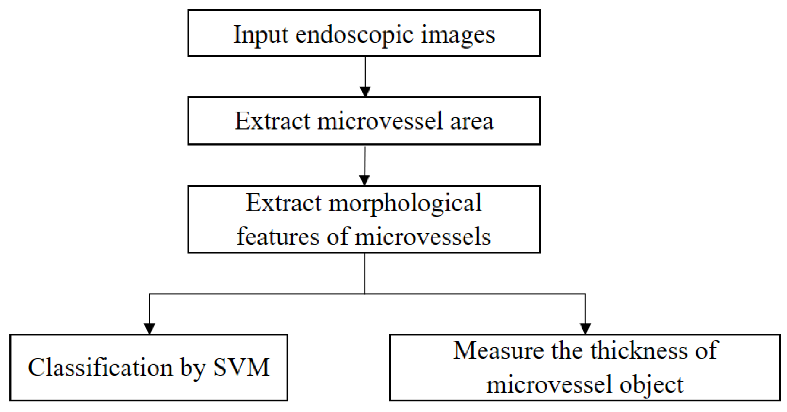
3. Materials and Methods
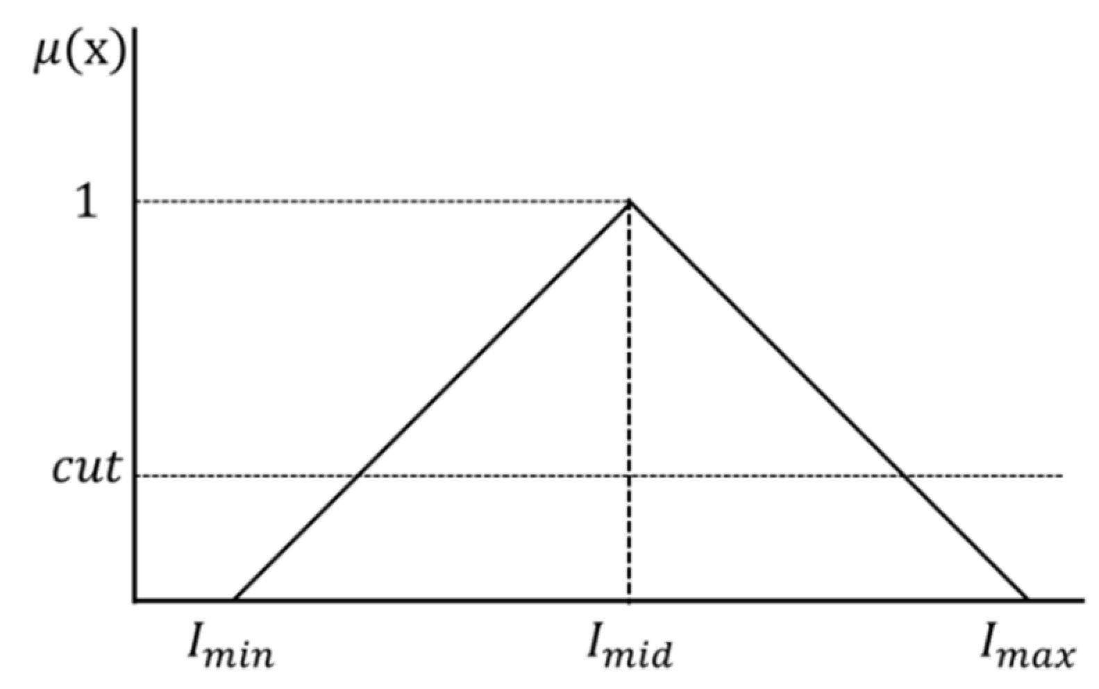
3.1. Contrast Enhancement of the ROI Using the Fuzzy Stretching Technique
3.2. Vein Area Extraction and Background Area Removal
3.2.1. Extraction of the Microvessel Candidate Region Using Niblack’s Binarization
3.2.2. Noise Elimination in the Vascular Boundary Region Using a Fast Fourier High-Frequency Filter
3.2.3. Removal of the Background Area Using the ART2 Algorithm
3.3. Extraction of Object Information from the Microvessel Area
Contour Tracing Algorithm
3.4. Extraction of Morphological Information from the Microvessels
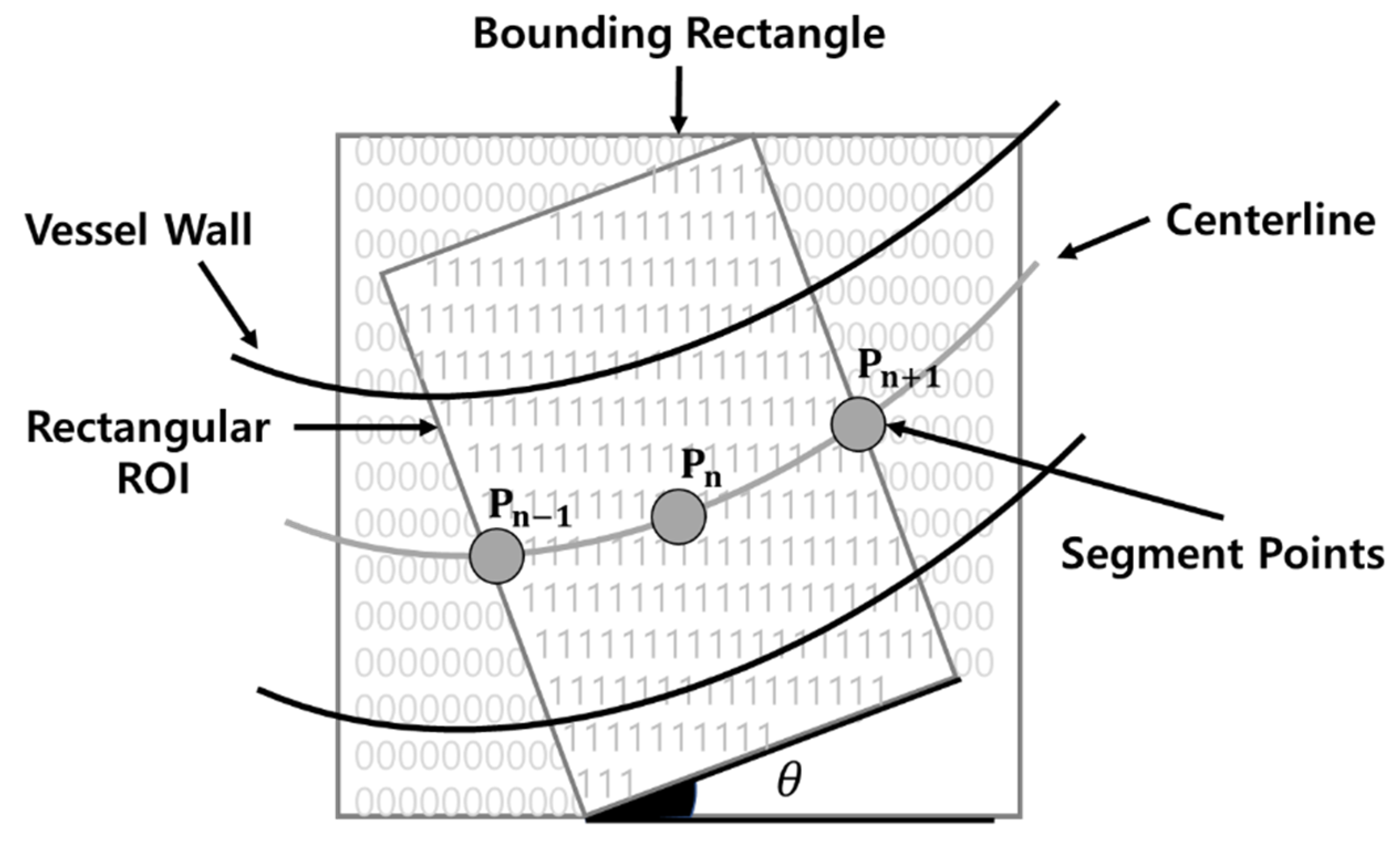
3.5. Microvessel Thickness Measurement
3.5.1. Extraction of the Microvessel Center Axis
3.5.2. Microvessel Thickness Measurement
4. Results
4.1. Environment
4.2. Experiment Results
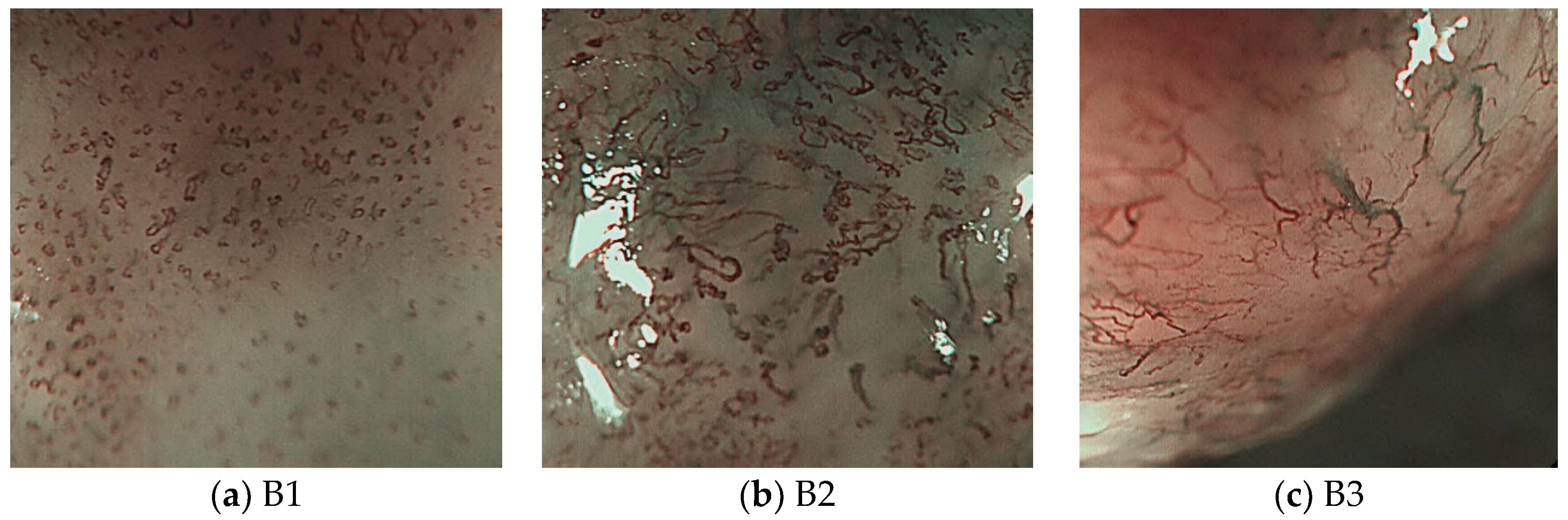
4.2.1. Classification Experiment Results for B1 and Non-B1 Types
4.2.2. Classification Experiment Results for the B2 and B3 Types
5. Discussion
Author Contributions
Funding
Conflicts of Interest
References
- Kumagai, Y.; Toi, M.; Kawada, K.; Kawano, T. Angiogenesis in superficial esophageal squamous cell carcinoma: Magnifying endoscopic observation and molecular analysis. Dig. Endosc. 2010, 22, 259–267. [Google Scholar] [CrossRef] [PubMed]
- Oyama, T.; Inoue, H.; Arima, M.; Omori, T.; Ishihara, R.; Hirasawa, D.; Takeuchi, M.; Tomori, A.; Goda, K. Prediction of the invasion depth of superficial squamous cell carcinoma based on microvessel morphology: Magnifying endoscopic classification of the Japan Esophageal Society. Esophagus 2017, 14, 105–112. [Google Scholar] [CrossRef] [PubMed]
- Kim, S.J.; Kim, G.H.; Lee, M.W.; Jeon, H.K.; Baek, D.H.; Lee, B.H.; Song, G.A. New magnifying endoscopic classification for superficial esophageal squamous cell carcinoma. World J. Gastroenterol. 2017, 23, 4416–4421. [Google Scholar] [CrossRef] [PubMed]
- Sato, H.; Inoue, H.; Ikeda, H.; Sato, C.; Onimaru, M.; Hayee, B.; Phlanusi, C.; Santi, E.G.R.; Kobayashi, Y.; Kudo, S. Utility of intrapapillary capillary loops seen on magnifying narrow-band imaging in estimating invasive depth of esophageal squamous cell carcinoma. Endoscopy 2015, 47, 122–128. [Google Scholar] [CrossRef] [PubMed]
- Arima, M.; Tada, T.; Arima, H. Evaluation of microvascular patterns of superficial esophageal cancers by magnifying endoscopy. Esophagus 2005, 2, 191–197. [Google Scholar] [CrossRef]
- Cortes, C.; Vapnik, V. Support-Vector networks. Mach. Learn. 1995, 20, 273–297. [Google Scholar] [CrossRef]
- Ebrahimi, M.A.; Khoshtaghaza, M.H.; Minaei, S.; Jamshidi, B. Vision-Based pest detection based on SVM classification method. Comput. Electron. Agric. 2017, 137, 52–58. [Google Scholar] [CrossRef]
- Sun, F.; Xu, Y.; Zhou, J. Active learning SVM with regularization path for image classification. Multimed. Tools Appl. 2016, 75, 1427–1442. [Google Scholar] [CrossRef]
- Yang, X.; Yu, Q.; He, L.; Guo, T. The one-against-all partition based binary tree support vector machine algorithms for multi-class classification. Neurocomputing 2013, 113, 1–7. [Google Scholar] [CrossRef]
- Gutierrez, M.A.; Pilon, P.E.; Lage, S.G.; Kopel, L.; Carvalho, R.T.; Furuie, S.S. Automatic measurement of carotid diameter and wall thickness in ultrasound images. Comput. Cardiol. 2002, 29, 359–362. [Google Scholar]
- Lowell, J.; Hunter, A.; Steel, D.; Basu, A.; Ryder, R.; Lee Kennedy, R. Measurement of retinal vessel widths from fundus images based on 2-D modeling. IEEE Trans. Med. Imaging 2004, 23, 1196–1204. [Google Scholar] [CrossRef] [PubMed]
- Kim, K.B.; Song, Y.S.; Park, H.J.; Song, D.H.; Choi, B.K. A fuzzy C-means quantization based automatic extraction of rotator cuff tendon tears from ultrasound images. J. Intell. Fuzzy Syst. 2018, 35, 149–158. [Google Scholar] [CrossRef]
- Saxena, L.P. Niblack’s binarization method and its modifications to real-time applications: A review. Artif. Intell. Rev. 2019, 51, 673–705. [Google Scholar] [CrossRef]
- Samorodova, O.A.; Samorodov, A.V. Fast implementation of the Niblack binarization algorithm for microscope image segmentation. Pattern Recognit. Image Anal. 2016, 26, 548–551. [Google Scholar] [CrossRef]
- Broughton, S.; Bryan, K. Discrete Fourier Analysis and Wavelets: Applications to Signal and Image Processing; Wiley-Interscience: Hoboken, NJ, USA, 2008. [Google Scholar]
- Park, J.; Song, D.H.; Han, S.S.; Lee, S.J.; Kim, K.B. Automatic extraction of soft tissue tumor from ultrasonography using ART2 based intelligent image analysis. Curr. Med. Imaging 2017, 13, 447–453. [Google Scholar] [CrossRef]
- Kim, K.B.; Kim, S. A passport recognition and face verification using enhanced fuzzy ART based RBF network and PCA algorithm. Neurocomputing 2008, 71, 3202–3210. [Google Scholar] [CrossRef]
- Olsen, M.A.; Hartung, D.; Busch, C.; Larsen, R. Convolution approach for feature detection in topological skeletons obtained from vascular patterns. In Proceedings of the 2011 IEEE Workshop on Computational Intelligence in Biometrics and Identity Management (CIBIM), Paris, France, 11–15 April 2011; pp. 163–167. [Google Scholar]
- Kang, C.; Huo, Y.; Xin, L.; Tian, B.; Yu, B. Feature selection and tumor classification for microarray data using relaxed Lasso and generalized multi-class support vector machine. J. Theor. Biol. 2019, 463, 77–91. [Google Scholar] [CrossRef] [PubMed]
- Everson, M.; Herrera, L.; Li, W.; Luengo, I.M.; Ahmad, O.; Banks, M.; Magee, C.; Alzoubaidi, D.; Hsu, H.M.; Graham, D.; et al. Artificial intelligence for the real-time classification of intrapapillary capillary loop patterns in the endoscopic diagnosis of early oesophageal squamous cell carcinoma: A proof-of-concept study. United Eur. Gastroenterol. J. 2019, 7, 297–306. [Google Scholar] [CrossRef] [PubMed]
- Guo, L.; Xiao, X.; Wu, C.; Zeng, X.; Zhang, Y.; Du, J.; Bai, S.; Xie, J.; Zhang, Z.; Li, Y.; et al. Real-Time automated diagnosis of precancerous lesions and early esophageal squamous cell carcinoma using a deep learning model (with videos). Gastrointest. Endosc. 2020, 91, 41–51. [Google Scholar] [CrossRef]
- Jung, H.K. Epidemiology of and risk factors for esophageal cancer in Korea. Korean J. Helicobacter Up. Gastrointest. Res. 2019, 19, 145–148. [Google Scholar] [CrossRef]


| Step 1 | In a binary image, start contour tracing when an object is found while moving sequentially from the top-left pixel. The tracing direction is indicated as d, and the first contour tracing direction is set to d = 0. |
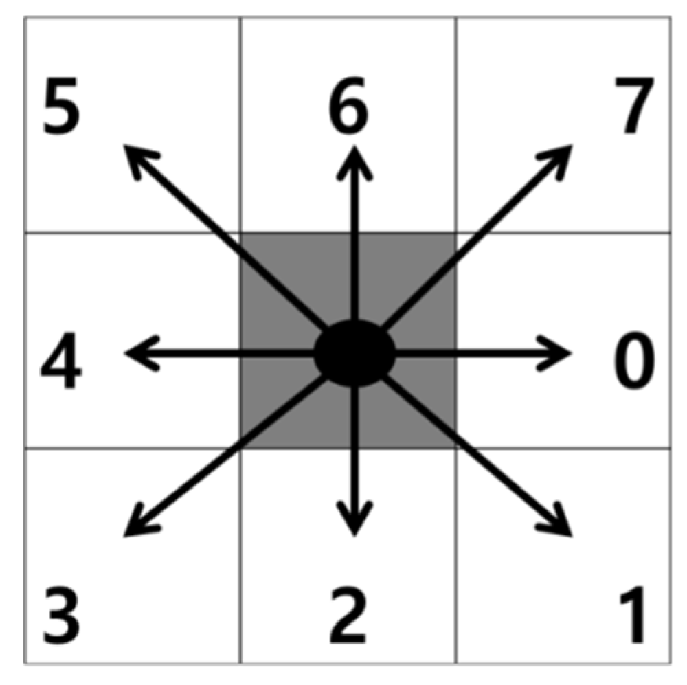
| Step 2 | Determine the existence of an object while rotating along the tracing direction as shown in Figure 11. |
| Step 3 | If an object exists, move to the position and set the tracing direction to d = d − 2. Determine the next direction of movement by rotating counterclockwise and then proceed to Step 2. |
| Step 4 | If there is no object in the moving direction, set d = d + 1 and proceed to Step 2. If there is no object in all directions, stop contour tracing because the object has only one pixel. |
| Step 5 | Stop contour tracing if the tracing coordinate is identical to the starting coordinate and the moving direction is 0. |
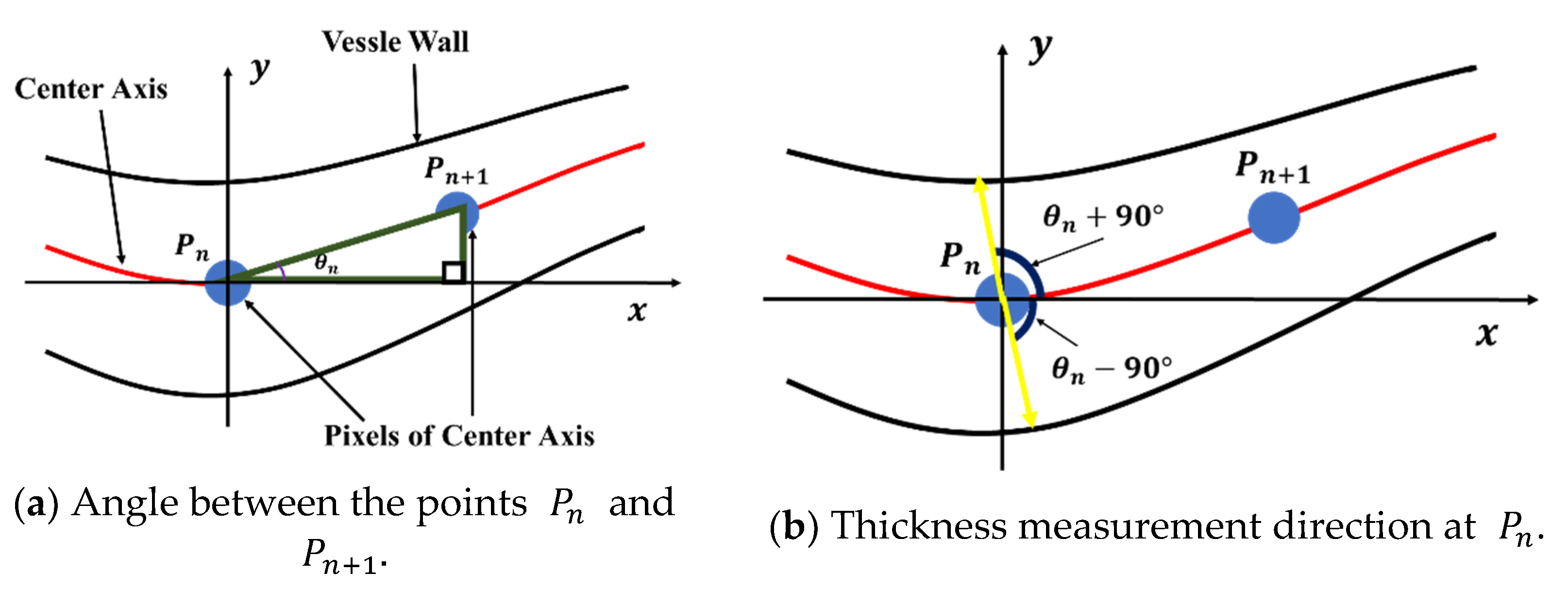
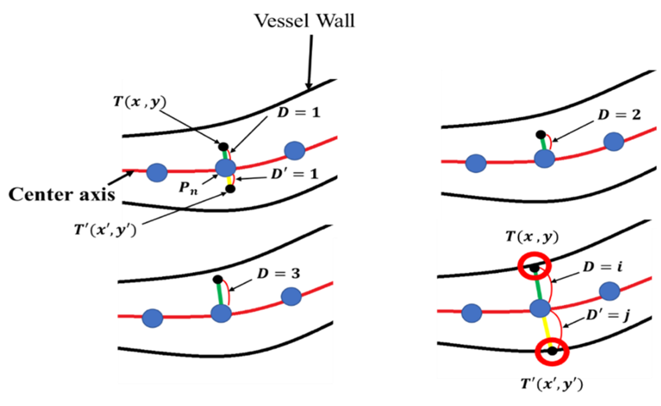
| Step 1 | Set the initial position at a distance D from , defined as . |
| Step 2 | Check if the value encounters the microvessel wall. |
| Step 3 | If reaches the microvessel wall, stop searching and proceed to Step 4 to end the algorithm or increase the length of D by 1 in Step 1 and repeat Step 2. |
| Step 4 | End. |
| True positive | 35 |
| True negative | 60 |
| False positive | 7 |
| False negative | 12 |
| True positive | 14 |
| True negative | 34 |
| False positive | 14 |
| False negative | 5 |
| True positive | 14 |
| True negative | 35 |
| False positive | 13 |
| False negative | 5 |
© 2020 by the authors. Licensee MDPI, Basel, Switzerland. This article is an open access article distributed under the terms and conditions of the Creative Commons Attribution (CC BY) license (http://creativecommons.org/licenses/by/4.0/).
Share and Cite
Kim, K.B.; Yi, G.Y.; Kim, G.H.; Song, D.H.; Jeon, H.K. Intelligent Computer-Aided Diagnostic System for Magnifying Endoscopy Images of Superficial Esophageal Squamous Cell Carcinoma. Appl. Sci. 2020, 10, 2771. https://doi.org/10.3390/app10082771
Kim KB, Yi GY, Kim GH, Song DH, Jeon HK. Intelligent Computer-Aided Diagnostic System for Magnifying Endoscopy Images of Superficial Esophageal Squamous Cell Carcinoma. Applied Sciences. 2020; 10(8):2771. https://doi.org/10.3390/app10082771
Chicago/Turabian StyleKim, Kwang Baek, Gyeong Yun Yi, Gwang Ha Kim, Doo Heon Song, and Hye Kyung Jeon. 2020. "Intelligent Computer-Aided Diagnostic System for Magnifying Endoscopy Images of Superficial Esophageal Squamous Cell Carcinoma" Applied Sciences 10, no. 8: 2771. https://doi.org/10.3390/app10082771
APA StyleKim, K. B., Yi, G. Y., Kim, G. H., Song, D. H., & Jeon, H. K. (2020). Intelligent Computer-Aided Diagnostic System for Magnifying Endoscopy Images of Superficial Esophageal Squamous Cell Carcinoma. Applied Sciences, 10(8), 2771. https://doi.org/10.3390/app10082771