HyCAD-OCT: A Hybrid Computer-Aided Diagnosis of Retinopathy by Optical Coherence Tomography Integrating Machine Learning and Feature Maps Localization

Abstract

Optical Coherence Tomography (OCT) imaging has major advantages in effectively identifying the presence of various ocular pathologies and detecting a wide range of macular diseases. OCT examinations can aid in the detection of many retina disorders in early stages that could not be detected in traditional retina images. In this paper, a new hybrid computer-aided OCT diagnostic system (HyCAD) is proposed for classification of Diabetic Macular Edema (DME), Choroidal Neovascularization (CNV) and drusen disorders, while separating them from Normal OCT images. The proposed HyCAD hybrid learning system integrates the segmentation of Region of Interest (RoI), based on central serious chorioretinopathy (CSC) in Spectral Domain Optical Coherence Tomography (SD-OCT) images, with deep learning architectures for effective diagnosis of retinal disorders. The proposed system assimilates a range of techniques including RoI localization and feature extraction, followed by classification and diagnosis. An efficient feature fusion phase has been introduced for combining the OCT image features, extracted by Deep Convolutional Neural Network (CNN), with the features extracted from the RoI segmentation phase. This fused feature set is used to predict multiclass OCT retina disorders. The proposed segmentation phase of retinal RoI regions adds substantial contribution as it draws attention to the most significant areas that are candidate for diagnosis. A new modified deep learning architecture (Norm-VGG16) is introduced integrating a kernel regularizer. Norm-VGG16 is trained from scratch on a large benchmark dataset and used in RoI localization and segmentation. Various experiments have been carried out to illustrate the performance of the proposed system. Large Dataset of Labeled Optical Coherence Tomography (OCT) v3 benchmark is used to validate the efficiency of the model compared with others in literature. The experimental results show that the proposed model achieves relatively high-performance in terms of accuracy, sensitivity and specificity. An average accuracy, sensitivity and specificity of 98.8%, 99.4% and 98.2% is achieved, respectively. The remarkable performance achieved reflects that the fusion phase can effectively improve the identification ratio of the urgent patients’ diagnostic images and clinical data. In addition, an outstanding performance is achieved compared to others in literature.

1. Introduction

Optical Coherence Tomography (OCT) imaging is a type of optical biopsy. It is used to view and capture small changes in retina. It generates cross sectional 3D images by measuring the echo time delay or the magnitude of back reflected light [1]. Compared to traditional regular retinal fundus examinations, OCT has major advantages in identifying the presence of various ocular pathologies. A wide range of macular diseases such as Macular Edema, Choroidal Neovascularization, Macular Hole, Pigment Epithelium Detachment and Central Serous Retinopathy can be detected by OCT [2]. OCT examinations can aid the detection of the previously mentioned disorders in an early stage. In OCT, cystic and sub retinal swellings are overt in early stages, while they remain undetectable in retinal fundus images [2]. In addition, OCT is noninvasive and quantifiable without pupil dilation. Hence, OCT scanning leads to a breakthrough in the screening, diagnosis and assessment of the necessity and efficacy of treatment for particular diseases. Nevertheless, a specialist is still required for the inspection and evaluation of the OCT findings, which creates burden and subsequent bottle necks in health care provision.

Alternative diagnostic and screening methods are needed to handle the existing bottlenecks. A lot of automated systems were recently developed to give clinical-decision support for medical imaging and to speed up the diagnostic process [3]. The incorporation of machine learning (ML) techniques for screening and diagnosis has a massive prospect in advancing health care provision, through timely and accurate decision making. Machine learning has made a revolution in developing these automated systems by implementing robust algorithms and by detecting features that help in classification of different diseases within a small time and within an acceptable accuracy [4].

In this paper, a computer-aided OCT diagnostic system is proposed for classification of Diabetic Macular Edema (DME), Choroidal Neovascularization (CNV) and drusen disorders, while separating them from Normal OCT images. The proposed model HyCAD presents a hybrid learning system, which integrates deep learning and traditional ML for effective diagnosis of retinal disorders. The proposed system assimilates a range of techniques including RoI localization, feature extraction and dimensionality reduction, followed by classification and diagnosis.

The contribution of the paper can be summarized as establishing a robust hybrid machine learning model for accurately diagnosing different retinal disorders such as CNV, DME and drusen. The model provides effective RoI localization and hand-crafted features generation. The fusion of automatically generated deep learning features and human articulated features noticeably improves the performance of pure deep learning architectures.

The paper is organized as follows: in Section 2, a medical background on retina anatomy in OCT is introduced. Section 3 gives an overall literature survey on OCT segmentation techniques and literature background on using machine learning in retinal diseases diagnosis based on OCT. Section 4 presents the dataset description and the applied data preprocessing. The proposed system architecture and the implemented models are detailed in Section 5. The results of different experimental scenarios are shown and discussed in Section 6. Finally, conclusions will be drawn in Section 7.

2. Medical Background: Retina Anatomy in OCT

The retina contains several layers with different thicknesses and intensities. Separating and determining the thickness of each layer are taken as vital markers in evaluating the health condition of the retina. The shape and width of the individual layers are considered two of the most important factors that reveal the current status or progress of a disease [5]. The layers may thicken or thin over the course of different diseases. Hence, many retinal diseases can be diagnosed through detecting irregularities in OCT images. Recently, there are many studies, which are conducted to analyze the OCT retinal images and to classify the healthy from diseased patients.

DME, CNV and drusen diseases are considered in this study. The anatomy of these diseases is portrayed and contrasted to normal anatomy in Figure 1. A brief description of each of the considered diseases in this study is given below.

Macular edema is the swelling of the central part of the retina [6]. It is considered one of the most common retinal disorders. Increased blood sugar levels, in people with diabetes, can damage the retinal blood vessels or result in tiny bulges protruding from the vessel walls, leaking or oozing fluid and blood into the retina. This leads to the serious eye complication called Diabetic Macular Edema (DME) [7], which may cause vision problems or blindness.

Another type of retinal disorder is Choroidal Neovascularization (CNV), it is the creation of new blood vessels in the choroid layer of the eye. Neovascular Degenerative maculopathy is commonly accompanied with extreme myopia, malignant myopic degeneration or age-related developments [8]. CNV is a major cause of visual loss.

Another type of retinal disorder is drusen. It is small yellow deposits of fatty proteins (lipids) that accumulate under the retina. The retina is a thin layer of tissue that lines the back of the inside of the eye, near the optic nerve. The retina contains light-sensing cells that are essential for vision [9]. Drusen are like tiny pebbles of debris that build up over time and can result in central vision loss. Central vision allows us to focus on details straight ahead [9].

The presence of overt changes in retina layers with various diseases in OCT images, encourage the development of diagnostic systems to differentiate between these diseases automatically. Computer aided diagnosis can support ophthalmologists with accurate timely decisions, thus leading to promoting health care provision.

3. Related Work

3.1. Literature Review on Retina Segmentation

In particular, segmentation has received considerable attention recently as it is an important step in aiding diagnosis since it helps determine the RoI. Ghorbel et al. [10] proposed a method for the segmentation of eight retinal layers in Heidelberg spectralis SD-OCT images. Global segmentation algorithms such as active contours and Markov random fields are used. In addition, a Kalman filter was designed. It is used to model the approximate parallelism between the photoreceptor segments [10].

A comparison between different edge detectors was conducted by Luo et al. [11]. They studied and compared the performance of canny edge detector [12,13], the two-pass method proposed by Bagci et al. [14] and Edgeflow technique [15]. All of these techniques were used with retinal OCT images to delineate the retinal layer boundaries. From the evaluation of the results, it was shown that the two-pass method outperforms the Canny detector and the EdgeFlow technique that is used with OCT images to delineate the retinal layer boundaries. In addition, the mean localization deviation metrics show that the smallest edge shifting problem is caused by the two-pass method. The study suggests that the two-pass method is the best one for retinal OCT boundary detectors.

In the work of Salarian et al. [16], a method that uses graph theory and the shortest path algorithm was presented to detect certain layers. The aim was to choose the RoI that could be used to distinguish normal cases from abnormal ones. They discovered that using changes in some parts, such as inner limiting membrane (ILM), retinal nerve fiber layer (RNFL) and retinal pigment epithelium (RPE), leads to separating these layers easily. The proposed technique was applied to all B-Scan images of 16 people, including low-quality images and some images with diseased eyes. The results were accurate according to manual segmentation of an expert.

Others such as Garvin et al. [17] proposed a method to segment five layers (NFL, GCL+IPL, INL+OPL, IS, OS) in OCT retinal images. The layers were identified using constructed geometric graph and computed a minimum cost closed set. This graph is constructed from the edge/regional information and a priori determined surface smoothness and interaction constraints.

3.2. Literature Review on Retina Disorder Classification Using OCT

Although the previous studies present effective segmentation techniques, there is a need to develop comprehensive diagnostic systems that emphasize RoI and perform disease classification. Such systems can help alleviate the burden on medical care systems.

Current automated diagnostic systems either use traditional ML techniques of feature extraction, segmentation and classification or utilize deep learning architectures with unprocessed images.

An example of these automated systems with OCT imaging can be found in the work of Srinivasan et al. [18]. It described an automated method for detecting retinal diseases using features extracted by Histogram of Oriented Gradients (HOG) techniques and SVMs to classify three classes namely DME, dry AMD and Normal. Their method does not rely on the segmentation of inner retinal layers; however, retinal flattening is performed. The proposed model achieved 100% for both DME and dry AMD classes and 86.67% for normal class. Another example of traditional approach is that of Alsaih et al. [19]. They proposed a pipeline model that generated a large set of extracted features using HOG and Local Binary Pattern (LBP) at four levels of the multiscale Gaussian lowpass image pyramid. These features were either reduced using Principle Component Analysis (PCA) or directly passed to SVM classifier, which was used to classify two classes: DME and normal. Their best model achieved an accuracy of 81%.

Naz et al. [1] addressed the problem of automatic classification of OCT images through SVM (leave one out) technique after image denoising and extraction of features from thickness profile and cyst spaces. This technique was based on extracting features from segmenting the retinal layer (ILM and choroid layer) and from the changes in thickness of these layers. Naz et al. [1] applied that technique for the identification of patients with DME versus normal subjects. The proposed model achieved an accuracy of 79.65%.

These traditional approaches [1,18,19], which employed hand-crafted features for the classifiers, were shown to obtain promising results. However, these approaches shared a common disadvantage, which is requiring abundant expert knowledge. Medical knowledge was needed to correctly detect retinal layers and/or changes in layers’ thickness [1] and/or assist in retinal flattening [18,19]. Such dependence on experts’ availability gives rise to another concern, which is having poor generalization to other domains [20]. Despite these limitations, hand-crafted features remain to provide intuitive information, which enables the needed analysis of the model [21]. Hence, the generation of hand-crafted features that are not heavily reliant on experts’ knowledge would provide the required balance of providing explanation of the model without being dependent on an expert. This balance would help mitigate the pressure on medical systems. In order to overcome these disadvantages, deep learning techniques were employed to perform embedded feature extraction implicitly. Awais et al. [22] used a deep learning architecture (VGG16) for extracting features from different layers of the network. Classifications were made using KNN and Decision Tree based on the extracted features. The model is used to classify two classes: DME and normal. The best model got an accuracy of 87.5%.

Perdomo et al. [23] proposed a new CNN architecture for OCT classification. The new CNN consists of two blocks, the first block contains four subblocks with convolutional layers and max pooling and the last block has two fully connected layers. The new CNN was evaluated with different learning rates, until it was able to correctly detect DME with a classification accuracy of 93.75% between two classes: DME and normal at learning rate 0.00001.

Motozawa et al. [24] developed a pipeline model consisting of two CNNs. The first is used to differentiate AMD class from normal class and the second CNN model is used to divide the AMD class into those with exudates and without exudates using transfer learning. The first CNN achieved an accuracy of 99% and the second one achieved an accuracy of 93.9%. Despite that the models attained high accuracies, the classification was limited to two classes which simplifies the problem. The work of Kermany et al. [4] established a diagnostic tool based on a deep learning framework for the screening of patients with common treatable blinding retinal diseases. They applied their approach on an OCT dataset [25] with four classes which are DME, CNV, DRUSEN, NORMAL. They used transfer learning inception model which achieved 96.1% average accuracy. Their approach demonstrated performance comparable to that of human experts in classifying age-related macular degeneration and diabetic macular edema. Using the same dataset, Li et al. [20] adopted a transfer learning VGG16 network that achieved an accuracy of 98.6%.

Both studies applied deep learning approaches [4,20] to classify four different classes including serious diseases (DME, CNV) and achieved promising results. However, the problem for deep learning models (CNNs) presented in the work of Kermany et al. and Li et al. [4,20] is that its sensitivity to urgent referrals classes (CNV/DME) is unsatisfactory. This is the main argue point against the approaches in the work of Kermany et al. and Li et al. [4,20]. Another common concern of deep learning architectures is the limited interpretability of the constructed models.

The incorporation of hand-crafted features can provide an adequate solution to deep learning issues. Hand-crafted features can offer complementary information that increase the understandability of the classification decision [26,27]. In addition, the use of hand-crafted features was shown to considerably improve the performance of pure deep learning approaches [28]. Recently, similar studies for image classification and recognition have shown that the integration of deep and traditional learning yield better performance. Examples of these studies include the work of Zhang et al. [29] for face recognition and Xie at al. [30] for lung nodule classification. Moreover, deep learning architectures in return can provide automated localization of the retinal RoI, which overcomes the need for an expert to aid in the specification of the RoI, required for traditional feature extraction.

In this paper, we propose a hybrid computer aided diagnosis (HyCAD) system based on OCT images using deep and traditional learning to attain high accuracy classifications and provide relative insight into the classification decision. In addition, HyCAD provides automated RoI localization which helps advance the diagnosis process.

4. Dataset Description

4.1. Data Acquisition and Labeling

The current study uses a benchmark dataset which consists of 109,312 retinal OCT images. The dataset was selected from 207,130 retinal OCT images for 5319 adult patients taken between 2013 and 2017. The 207,130 retinal OCT images were collected from retrospective cohorts from the Shiley Eye Institute of the University of California San Diego, the California Retinal Research Foundation, Medical Center Ophthalmology Associates, the Shanghai First People’s Hospital and the Beijing Tongren Eye Center [20,25].

Two retinal specialists provided the class labels for the images. Four class labels were available CNV, DME, DRUSEN, NORMAL) as shown in Figure 2. Furthermore, only 109,312 out of 207,130 images were clearly distributed between these classes by the agreement of the two retinal specialists and formed the dataset while the other images contained severe artifacts. The dataset is divided into 108,312 images as training set and 1000 images as testing set, according to Li et al. [20]. The distribution of the classes within the training set is illustrated in

Table 1. Training dataset class distribution.

Training Dataset				Total
Urgent Referrals Group		Nonurgent Referrals Group
CNV	DME	DRUSEN	NORMAL
37,206	11,349	8617	51,140	108312
34.35%	10.48%	7.96%	47.22%	100%

, where both classes: DME and DRUSEN, present a small percentage of the training set and can be considered to impose the challenges of minority classes on our classification problem [4]. The testing set is sampled to be of equal distribution for all classes as illustrated in

Table 2. Testing dataset class distribution.

Testing Dataset				Total
Urgent Referrals Group		Nonurgent Referrals Group
CNV	DME	DRUSEN	NORMAL
250	250	250	250	1000
25%	25%	25%	25%	100%

.

The classes are categorized as Urgent referrals and Nonurgent referrals groups. The CNV and DME classes represent the Urgent referrals group, where patients need to be transferred to an ophthalmologist in time for definitive anti-VEGF treatment [4,20]. The referral is urgent in this case because if the treatment is delayed, it would almost cause irreversible vision impairment and even lead to blindness. The Nonurgent referrals group, represented by DRUSEN and NORMAL classes, does not need immediate Urgent referral from an ophthalmologist [4,20].

4.2. Image Preprocessing

A range of preprocessing steps are applied to the dataset to limit the processing system requirements and to increase the robustness of the models.

First, individual cross-sectional tomography (B-scans) in the SD-OCT volume are denoised using the sparsity-based block matching and 3D-filtering (BM3D) denoising method which reduces the speckle noise. It is the filter from the nonlocal means class that looks for local neighborhoods of similar shapes and puts them into a 3D matrix [31].

The applied BM3D filter noticeably reduces the speckle noise in images, as can be seen in Figure 3. Noise reduction helps in achieving good performance metrics.

Second, images are streamed in batches to avoid system crash due to RAM overloading, and this is because of the memory limitations. Memory limitations come from training models using a RAM size of small bandwidth compared to the large dataset used in training (108,312 images) and the large size of our deployed CNN architecture. To solve this problem, our data is partitioned into batches of 32 images and the training data was transferred batch by batch from the hard disk to RAM during training. After the training of each batch ends, it is discarded, and a new batch of images is generated and stored in RAM. So, each training epoch will have 3385 iterations (equal to number of training dataset/batch size). This technique allows us to train our large training set without RAM overflowing.

Data Augmentation is applied for each batch. Rotation by range from 0 to 30 degrees, horizontal flipping and shifting by range between 0 and 30% from left, right, up and down is applied randomly on each batch of images in each epoch to allow deep learning architectures to train on different orientations of input image, thus improving the robustness of the system. After that, all the images are resized to 200 × 200 pixels.

Each pixel value is normalized to process all images in the same manner because some images may have high pixel range that could cause stronger loss and low pixel range that could cause weaker loss. Additionally, high pixel range will have a large number of votes to determine how to update weights. So, if the values of intensities are normalized to avoid discrepancy in image processing caused by different pixel ranges, this could decrease the gap and make a fair competition in votes between high pixel range and low pixel range.

5. The Proposed HyCAD System: Hybrid Computer-Aided Diagnosis of Retinopathy Applying Deep and Traditional Machine Learning on OCT Images

In this section, the proposed model architecture will be introduced, with an illustration of the phases’ description. The proposed model utilizes modified variant of an existing deep learning architecture, namely VGG16, with OCT images for efficient diagnosis of retina disorders. The proposed deep learning architecture modifications aim at improving the performance of the standard basic architectures in terms of attained accuracy and training time requirements. The implemented architectures provide RoI localization and feature generation. Hand-crafted features are generated from the RoI that is extracted by the deep learning architecture. Afterwards, both CNN-based features and hand-crafted features are merged and input to the dense layer. Diagnosis is produced based on the classification output by the dense layer. The proposed system architecture is shown in Figure 4.

5.1. Norm-VGG16 Deep Learning Architecture

One of the most prominent deep learning architectures is VGGs Network. VGG16 [32] architecture is utilized for its known superior performance, for example, compared to other models like AlexNet [33]. This may be attributed to its small kernel size (3 × 3) and more trainable parameters, which helps increase the depth of CNN without the problem of gradient loss in deep CNNs. A set of modifications to the standard VGG network architecture are proposed to create Norm-VGG16 Network variant architecture that enhances the performance of the basic architecture.

First, the number of convolution layers is increased from 13 layers in standard VGG to 16 convolution layers. Each of the added layers has a kernel of size 3 × 3 and stride = 1. The pipeline of the convolution layers starts with first layer of size 200 × 200 and is convolved by 64 (3 × 3) kernels. The ending layer of the pipelined convolution layers has 512 (3 × 3) kernel with output of size 3 × 3. Between each group of convolution layers there is a max pooling layer of size (2 × 2) to down sample the feature tensor to reduce overfitting. The second applied modification is adding a global average pooling layer followed by a dense layer to reduce the overfitting of CNN. The dense layer has an output of four neurons representing the four classes of our dataset.

Another enhancement to the standard architecture is adding L2 kernel regularization to limit overfitting. The added regularization is shown in Figure 5 at the last dense layer. Kernel regularization was first added in different layers, but the best performance is attained by the variant scenario implementing L2 kernel regularization at the dense layer (last layer). The value of the hyperparameter of L2 regularizer, which determines the relative importance of the regularization component compared to the loss component, is set to 0.01.

L2 regularizer puts a constraint on the complexity of a network by giving a small value to its weights, which makes the distribution of weights regular. This is done by the increasing loss function of the network, which has large weights [34].

To explain how the regularizer works, a training function ŷ: f(x) should be first defined as a function that maps an input vector x to output ŷ where ŷ is predicted value for actual value y. The loss between ŷ (f(x)) and y can be defined for one sample x_i with corresponding target y_i. Loss (L) can be computed as L((y_i), ŷ_i) = L (f(x_i), y_i) [35]. For all input samples x_i ……. x_n. The sum of all loss functions between each input x_i and its corresponding output ŷ is minimized as given in Equation (1).

$$\underset{\hspace{1em}\hspace{1em}\mathrm{f}}{\min }{\displaystyle \sum }_{i=1}^{n}L{\left(f\left(x_i\right),y_i\right)}^{ }$$

(1)

The regularizer (R(f)) is added to the loss equation to increase the training loss to decrease overfitting as shown in Equation (2).

$$L\left(f\left(x_i\right), y_i\right)={\displaystyle \sum }_{i=1}^n{L}_{losscomponent}\left(f\left(x_i\right),y_i\right)+\lambda R{\left(f\right)}^{ }$$

(2)

where λ is a hyperparameter that determines the relative importance of the regularization component compared to the loss component [35]. We choose our λ = 0.01. From Equation (1) and Equation (2), minimization after adding the regularization would occur to both the component of loss and the regularization component. Different values for λ are tested in the range between 0 and 1 (0.001, 0.01, 0.02, 0.1, etc.) according to the commonly used values in literature [34,35]. The best results are obtained at λ = 0.01.

The L2 regularization is a type of regularization that is proportional to the square of the value of the weight coefficients (the L2 norm of the weights) [36] as shown in Equation (3).

$$R\left(f\right)={{\displaystyle \sum }}_{f i=1}^n{w}_i^2$$

(3)

By substituting Equation (3) into Equation (2), L2 regularization Equation (4) is generated

$$L\left(f\left(x_i\right), y_i\right)={\displaystyle \sum }_{i=1}^n{L}_{losscomponent}\left(f\left(x_i\right),y_i\right)+\lambda {\displaystyle \sum }_{i=1}^n{w}_i^2$$

(4)

5.2. RoI Localization and Segmentation

The performance of deep learning is noteworthy. Nevertheless, a shortcoming of deep learning architectures is that they are considered as black boxes which do not provide any insight into the classification process. Therefore, in this phase the activation maps are generated by Norm-VGG16 for our classes to visualize and localize the areas used for classification. The activation maps highlight the focus areas, from which most of the CNN-based features were extracted.

In order to generate discriminative localization map, Gradient-weighted Class Activation Mapping (Grad-CAM) module [37] is used. The implemented Grad-CAM module structure is shown in Figure 6. Grad-CAM L^c_Grad-CAM ∈ R^u×v of width u and height v for any class c. The gradient of the score of the class c is computed before the SoftMax layer (y_c) with respect to feature maps A_k of a convolutional layer $\frac{\partial y^c}{\partial A^k}$. These gradients flowing back are global average pooled to obtain the neuron importance weights α^c_k as shown in Equation (5).

$${\propto }_k^c=\stackrel{\begin{array}{c}global \\ average pooling\end{array}}{\overbrace{\frac{1}{Z} {\displaystyle \sum }_i {\displaystyle \sum }_j }}\underset{\begin{array}{c}gradiants via\\ backpropagation\end{array}}{\underbrace{\frac{\partial y^c}{\partial A_{ij}^k}}}$$

(5)

This weight α_c^k represents a partial linearization of the deep network downstream from A and captures the “importance” of feature map k for a target class c. After that a weighted combination of forward activation maps takes place. RELU is applied on the combination of feature maps. RELU is used to emphasize the positive influencer pixels whose intensity should be increased in order to increase y^c for a certain class and remove the negative influencer pixels that are likely to belong to other categories in the image as shown in Equation (6).

$$L_{Grad-CAM}^c=ReLU \underset{linear combination}{\underbrace{\left( {\displaystyle \sum }_k{\propto }_k^c{A}^k\right)}}$$

(6)

The RELU helps in highlighting the positive influencer pixels in the localization maps and avoid highlighting the negative influencer pixels, which achieve better localization [37].

The generated heat maps (activation maps) seem to clearly portray the RoIs used in classification, which can be considered as implicit segmentation. Thus, they provide transparency of the model, which is required in medical diagnosis. The generated heat maps for all the four classes are shown in Figure 7, where the activation maps clearly mark the RoI.

The shown samples of the activation maps clearly mark the RoI that can be used in classification and feature generation. As shown in Figure 8, a binary mask is generated for each image from the RoI and the corresponding image is segmented using this binary mask.

The binary masks are generated based on the heat maps output by the Norm-VGG16 deep learning architecture. The heat maps highlight the RoI, which allow the generation of binary masks. Simple global thresholding [38,39] is used, where a histogram is plotted for each heat map and the respective threshold value is determined. The threshold value is selected per individual heat map such that red and yellow areas in the heat map are used to create the mask (emphasizing the localized RoI region) as shown in Figure 9. The global threshold value is used to generate the binary mask.

5.3. Hand-Crafted Feature Generation

After RoI localization and cropping, a set of spatially articulated features are generated. Before generation, the cropped part of the image is resized to 64 × 64. Then, HOG and DAISY feature descriptors were generated.

HOG descriptors are calculated by normalizing colors then dividing the image into blocks and each block is divided into smaller units called cells. Each cell contains number of pixels (pixel intensities). First, the gradient magnitude and direction of each cell’s pixel intensities is calculated. If (x, y) is assumed as a pixel intensity, then gradient magnitude is calculated from Equation (7) and gradient angle is calculated using Equation (8) [40,41].

$$G\left(x,y\right)=\sqrt{\left(G_x{\left(x,y\right)}^2+G_y{\left(x,y\right)}^2\right)}$$

(7)

$$\theta \left(x,y\right)=\arctan {\left(\frac{G_{y\left(x,y\right)}}{G_{x\left(x,y\right)}}\right)}^{ }$$

(8)

After calculating magnitude and angle, the HOG is calculated for each cell by calculating the histogram. Q bins for angles are chosen with unsigned orientation angles between 0 and 180. Afterwards, normalization is applied since different images may have different contrasts [40]. The pipeline of HOG can be shown in Figure 10. In our implementation, a [4 × 4] cell size, [2 × 2] cells per block and 9 orientation histogram bins creating 8100 features were used.

DAISY feature descriptor is an algorithm that generates low dimensional invariant descriptors that convert local image regions into low dimensional invariant descriptors, which can be used for matching and classification. DAISY feature descriptor is faster than GLOH and SIFT feature descriptors [42]. It can be computed efficiently at every pixel unlike SURF. For DAISY descriptors generation, eight orientation maps, G, are computed for each image. one for each quantized direction, where G (u, v) equals the image gradient at location (u, v) [42]. Gaussian kernels of different ∑ values convolve each orientation map several times to obtain convolved orientation maps for different sized regions [42]. If h_∑ (u, v) is the vector made of the values at location (u, v) in the orientation maps after convolution by a Gaussian kernel of standard deviation Σ as shown in Equation (9), after that, the If h_∑ (u, v) is normalized

$$h_{{{\displaystyle \sum }}^{}} \left(u,v\right)={\left[G_1^{{{\displaystyle \sum }}^{}} \left(u,v\right), \dots \dots \dots , G_8^{{{\displaystyle \sum }}^{}} \left(u,v\right) \right]}^T$$

(9)

where G₁^∑, G₂^∑…….G₈^∑ denote the Σ-convolved orientation maps. The vector is normalized and denoted by ĥ_∑ (u, v). To correctly represent the pixels near occlusions, the normalization is performed in each histogram independently because normalizing the descriptor as a whole would lead to the same point, which is close to occlusions, appearing different in two images. A complete explanation of calculating Full DAISY descriptor is given by Tola et al. [42].

5.4. Feature Fusion and Classification

A set of 512 CNN-based features are extracted per image from our Norm-VGG16 network architecture. The features are extracted from the global average pooling layer. These features are fused with the 8100-feature array of hand-crafted HOG descriptors and 400-feature array of hand-crafted DAISY, leading to a concatenated array size of 9012 features. The classification of these feature sets is done in batches. A Neural Network consisting of three dense layers is used to train these features with first layer of input size of 9012 inputs and 2048 neurons followed by a hidden layer of 512 neurons and the final layer contains four neurons with a SoftMax activation to normalize the distribution probability as shown in Figure 11. The model is trained using Adam optimizer with batch size 32 for 100 epochs.

5.5. Expermental Setup

Models implementation, training and results are done using Python language v3.7.6 (designed by Guido van Rossum and developed by Python Software Foundation, this version is released on December 2019) with Numpy v1.18.4 (Travis Oliphant), Tensorflow v2.1.0 (Google Brain team), Keras v2.3.1 (François Chollet) and OpenCV v4.2.0 (Intel Corporation, Willow Garage, Itseez) packages Experiments are conducted on Google Colab (free cloud service hosted by Google). Google Colab consists of 1xNvidia Tesla K80, 12.6 GB RAM and 320 GB Disk space.

All deep learning architectures are trained for 30 epochs from scratch using Adam optimizer with starting learning rate of 0.001 on the 108,312 training images. Inputs are divided into batches of size 32. Validation accuracy and cross-entropy loss are monitored for each epoch. In addition, the learning rate is reduced by factor of 0.2 for each three epochs without improvement in validation loss.

For the deep learning architectures, the best model is defined as having minimum validation loss, then it is stored and applied on the testing set. The best model Norm-VGG16 took about 12 h to be trained.

6. Results and Discussion

6.1. Performance Metrics

The following measures are used to evaluate the performance of trained models to decide which one has advantage over the others.

6.1.1. Confusion Matrix

It is a table that is used to visualize and describe the performance of a classification model on a testing set of data as shown in Figure 12. It is a summary of prediction results in a classification problem [43]. In confusion matrix, values of True Positive (TP), True Negative (TN), False Positive (FP) and False Negative (FN) are represented by assuming C_i one of the four classes in our dataset.

• TP (C_i.) = All the instance of C_i. that are classified as C_i.
• TN (C_i.) = All the non-Ci. instances that are not classified as C_i.
• FP (C_i.) = All the non-Ci. instances that are classified as C_i.
• FN (C_i.) = All the Ci instances that are not classified as C_i.

6.1.2. Accuracy (Acc)

It is measured by dividing the number of correctly labeled images by the total number of test images [4]. Equation (10) depicts single class accuracy measurements

$$Accuracy=\frac{TruePositive+True Negative}{True Positive+True Negative+False Positive+False Negative}$$

(10)

6.1.3. Sensitivity (Recall)

It is determined by dividing the total number of correctly classified Urgent referrals by total number of actual Urgent referrals [4]. Equation (11) depicts single class sensitivity measurements

$$Sensitivity=\frac{True Positive}{True Positive+False Negative}$$

(11)

6.1.4. Specificity (Sp)

It is determined by dividing the total number of correctly classified non-referrals by total number of actual Nonurgent referrals [4]. Equation (12) depicts single class specificity measurements

$$Specificity=\frac{True Negative}{True Negative+False Positive}$$

(12)

6.2. Experimental Results

In this section, the implemented experimental scenarios used for performance comparison and the corresponding results using the described performance evaluation metrics are described.

6.2.1. Experimental Scenarios

1. HyCAD Architecture

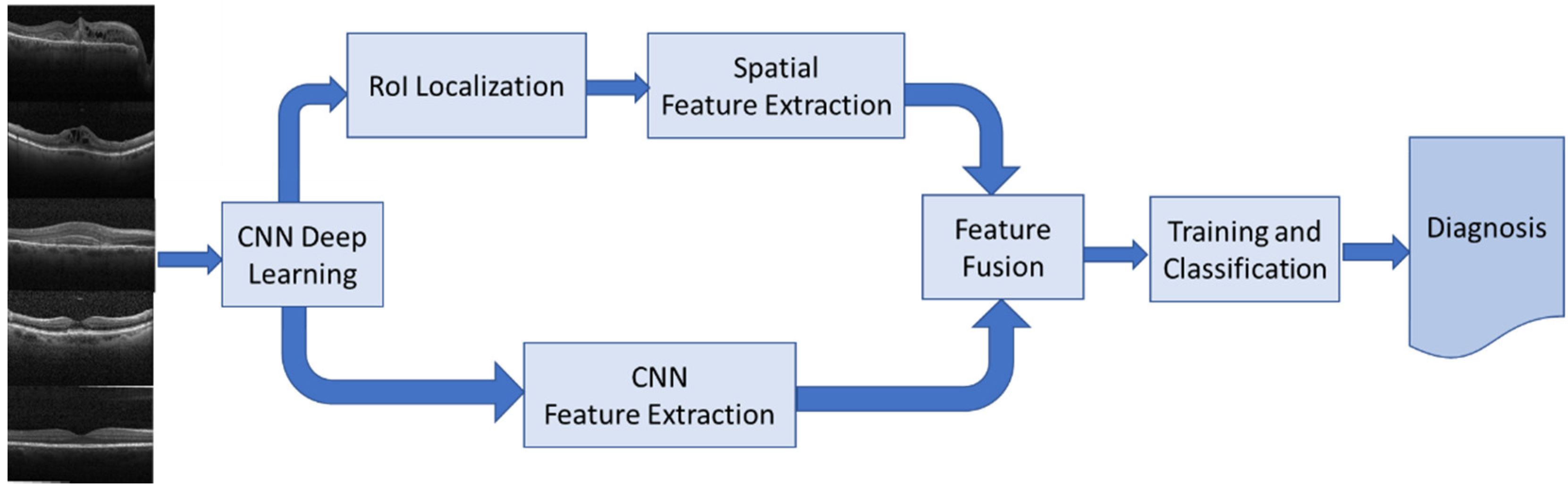
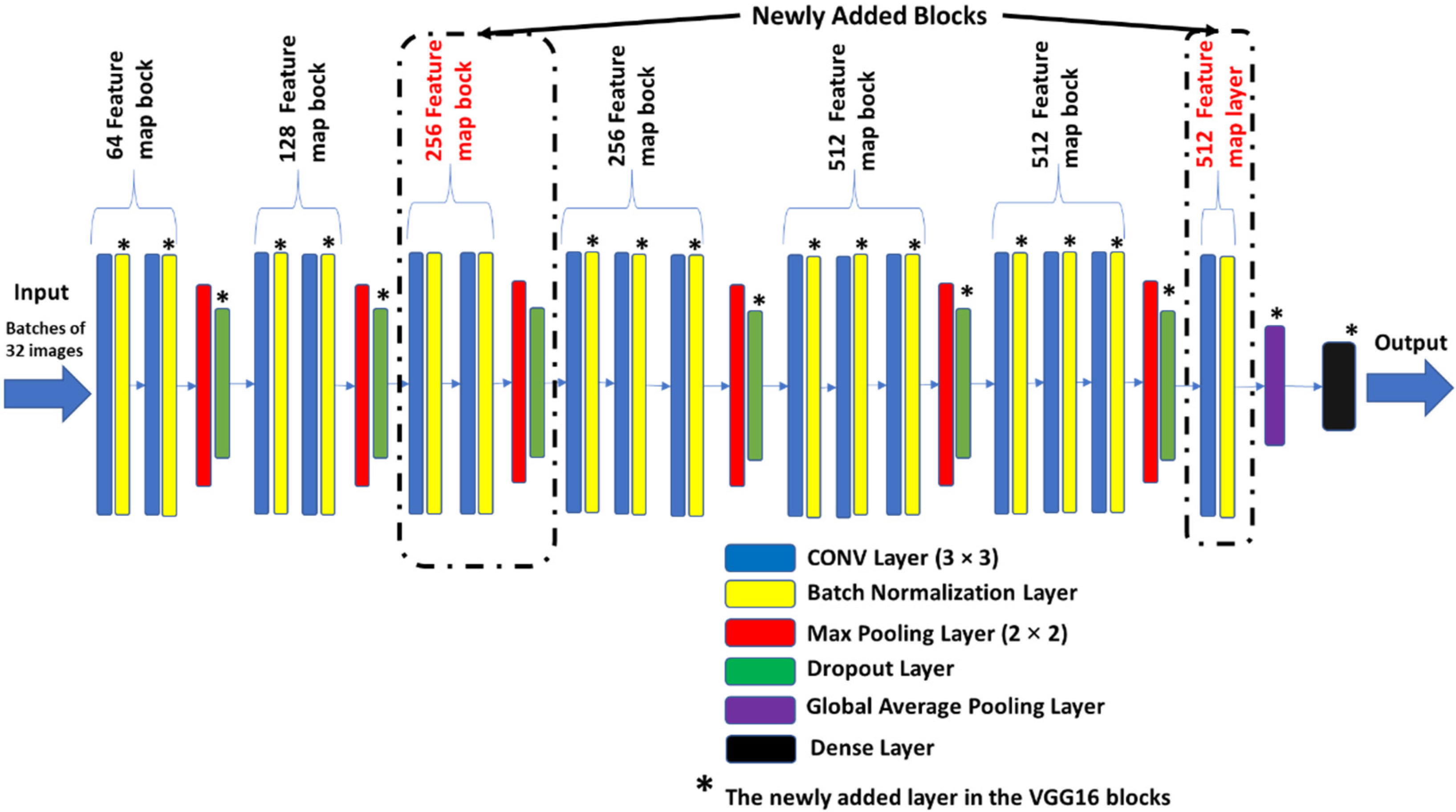
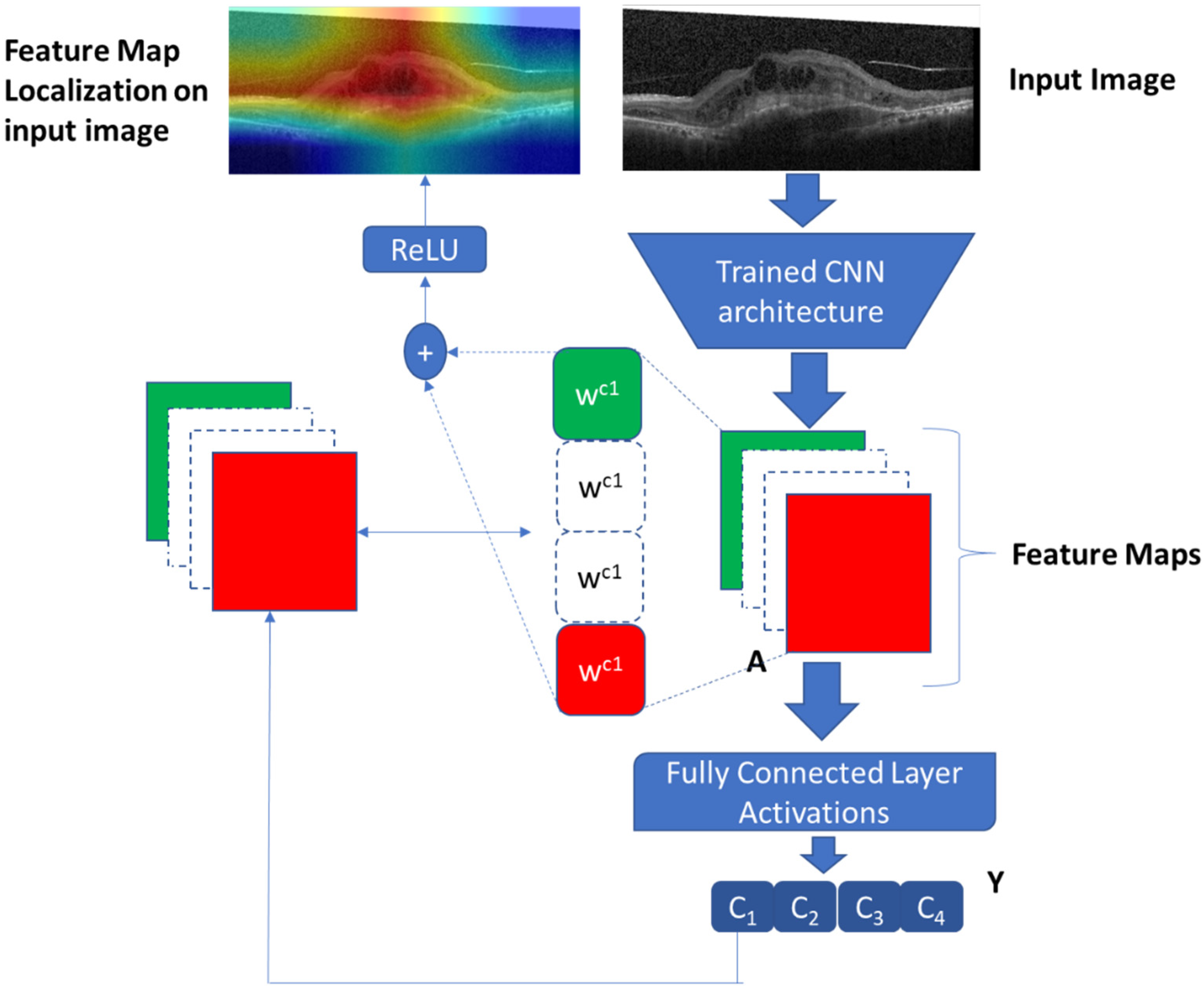
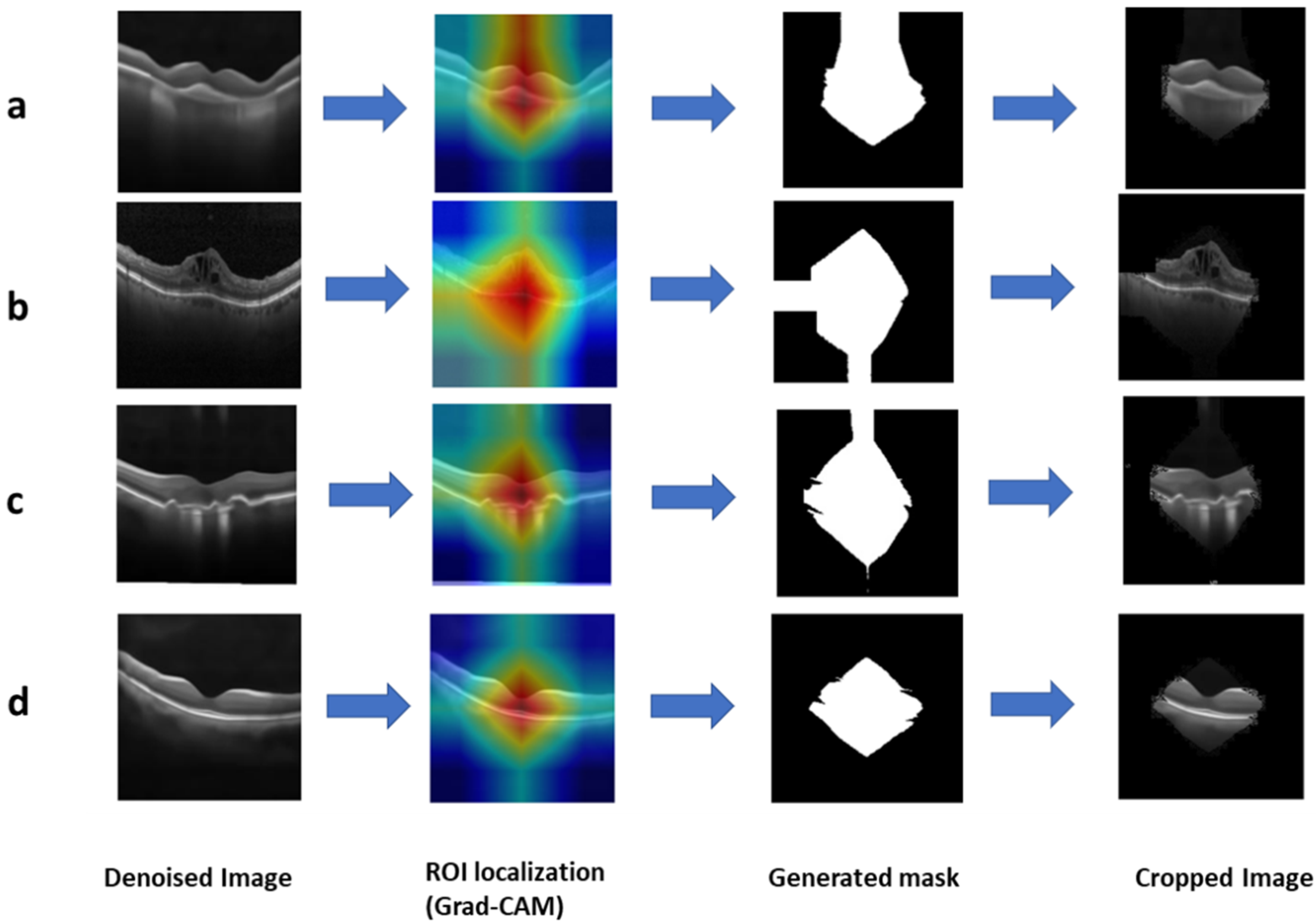
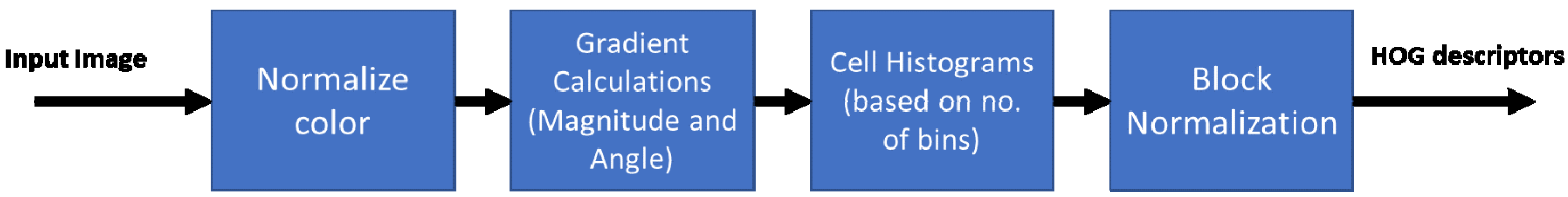
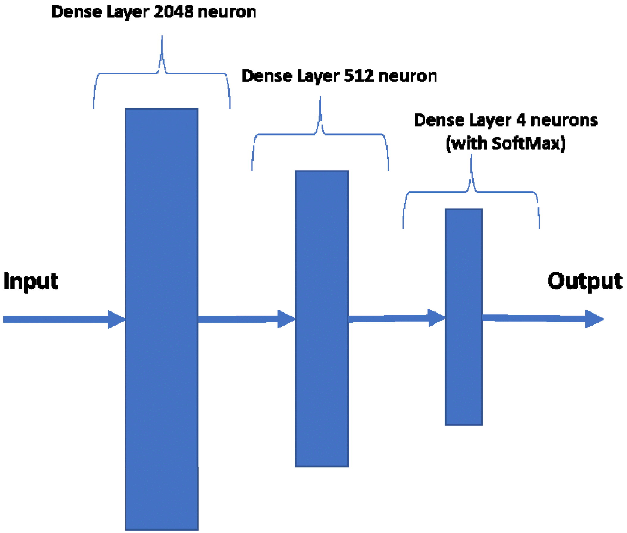
The proposed system architecture presented in Section 5 is applied to the dataset described in Section 4. Norm-VGG16 integrating kernel regularizer is trained on the dataset from scratch aiming at higher performance metrics. It is used for RoI generation and feature extraction. A set of 512 features are extracted from the global average pooling layer of the CNN network. The hand-crafted feature extraction methods, namely HOG and DAISY, when applied on the segmented RoI generated 8500 features. At the fusion stage of our HyCAD system, all the extracted features are fused and fed into a three sequential dense layer neural network for a classification decision.

2. Norm-VGG16 (kernel regularized) Deep Learning Architecture

In this scenario, the modified Norm-VGG16 Deep Learning architecture is applied on the OCT dataset. The performed classification is based solely on the CNN-based features. This scenario is presented to elucidate the merit of incorporating human articulated features on the performance of the system.

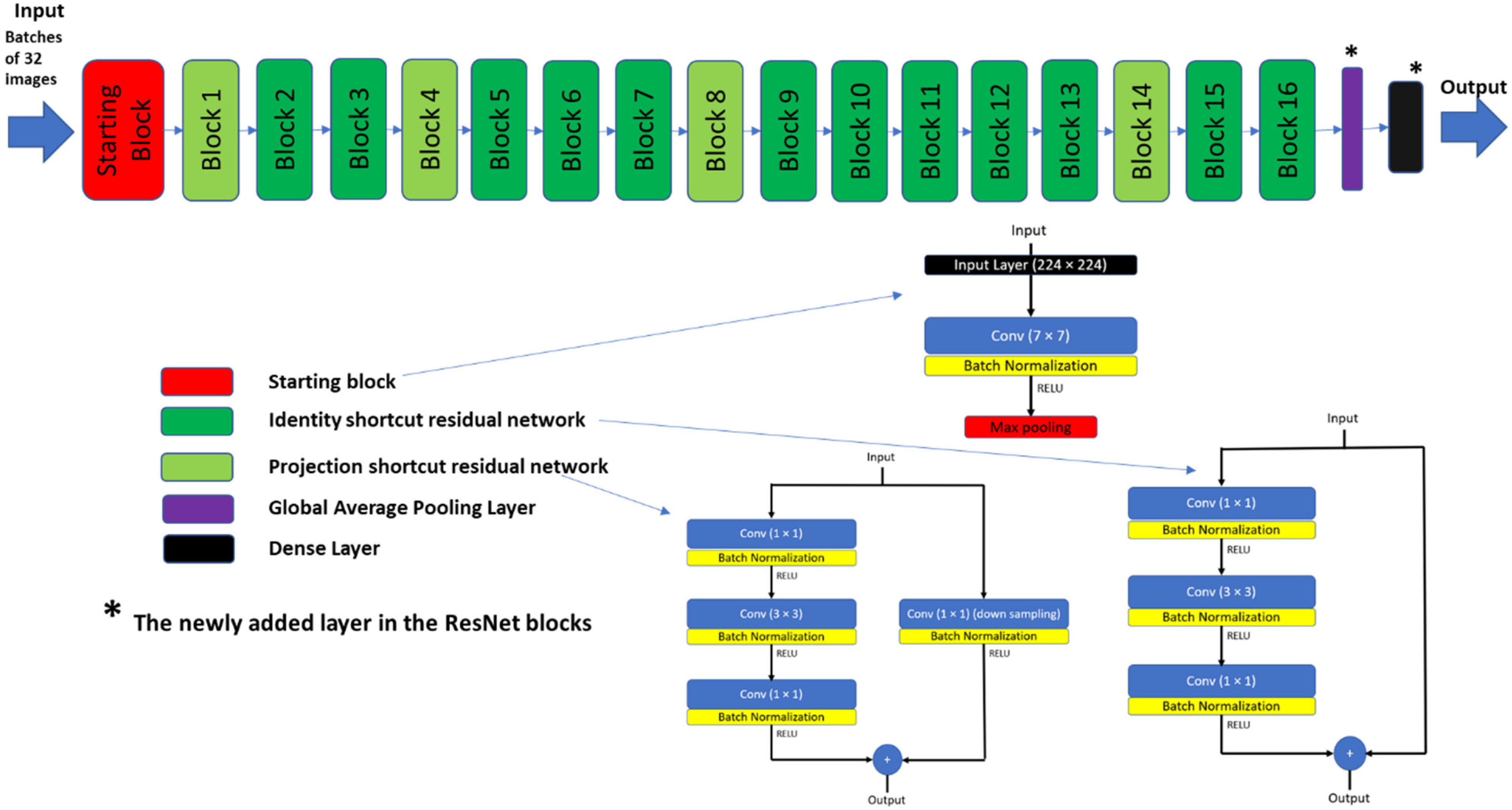
3. ResNet-50 Net (kernel regularized) Deep Learning Architecture

ResNets [32,44] can be considered one of the most applied deep learning architectures for image recognition and classification. ResNets include residual blocks which allow deeper network architecture to avoid information loss during training. In addition, it was shown to achieve lower validation loss compared to VGG16 on the ImageNet dataset [44]. Therefore, ResNet-50 architecture (shown in Appendix A) is chosen as one of our experimental scenarios, to compare its performance to the proposed HyCAD system. The ResNet-50 best model is modified by adding kernel regularization in the final dense layer.

In addition to these implemented experimental scenarios, the results of HyCAD are compared with the work of Kermany et al. [4] and Li et al. [20]. These were chosen as their results were reported on the same dataset using deep learning approaches and attained high results.

6.2.2. Classification Results

Our experimental results are shown in two folds. First, bootstrapping is adopted, and a limited set of results are reported to show the performance of HyCAD across several testing data partitions and investigate its stability relative to Norm-VGG16 and RESNET-50 and to clarify the impact of hand-crafted features’ fusion with deep learning architectures. In the second fold of experiments, elaborate results are reported on the same training and test percentages used by Kermany et al. [4] and Li et al. [20]. The results of the best run are displayed to be able to compare to Kermany et al. [4] and Li et al. [20].

1. Bootstrapping Experiments Fold

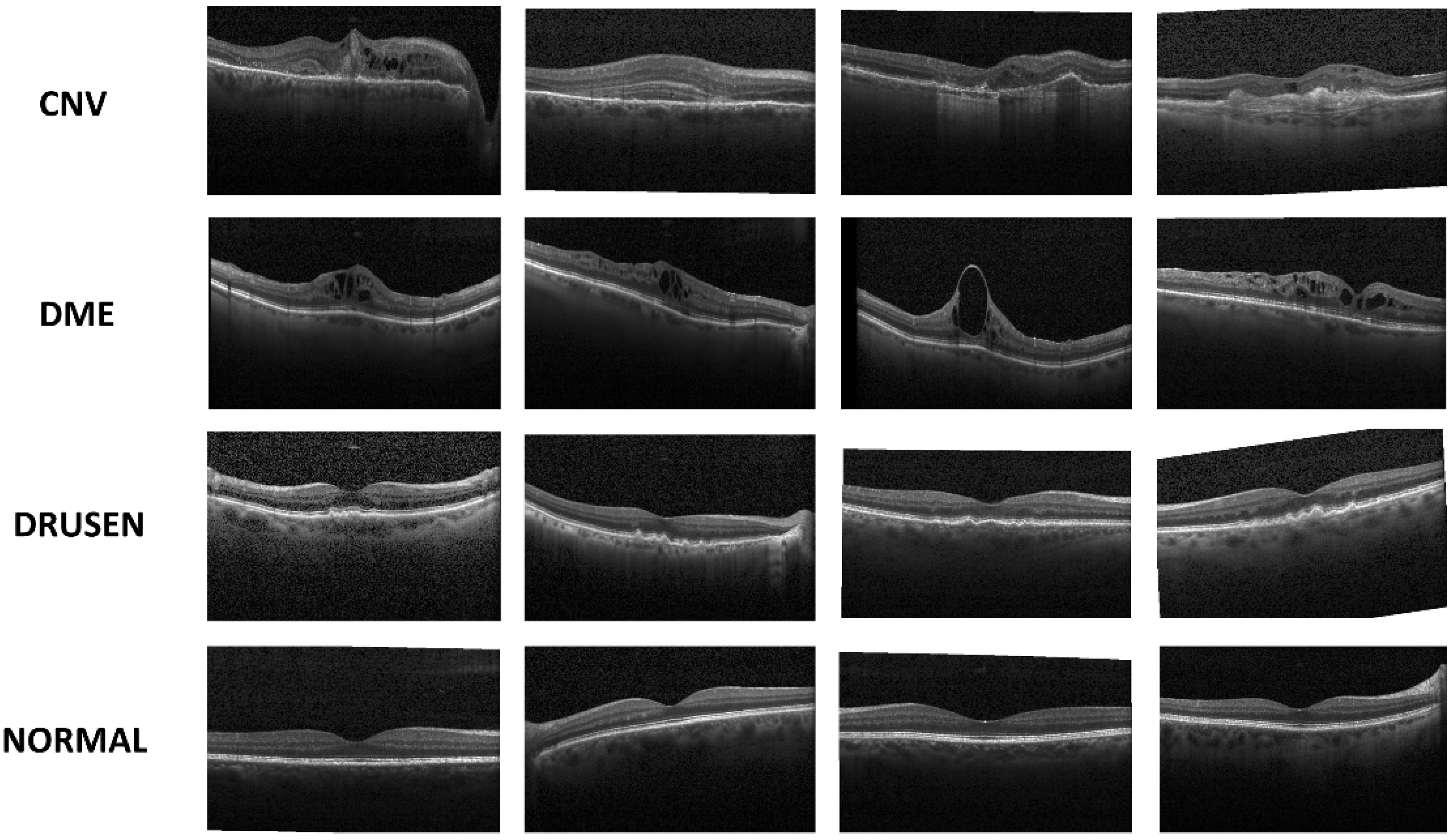
Ten bootstrapping experiments are conducted to evaluate the performance of the models at different boot strapped test partitions. In each experiment, the 109,312 images are shuffled and a random selection of 108,312 images is used as training dataset and the rest of the 1000 images are used as testing dataset. Each new partition tested on our implemented architectures (HyCAD, Norm-VGG16 integrating kernel regularizer and ResNet-50 integrating kernel regularizer) taking into consideration that the testing dataset is partitioned equally between four classes (CNV, DME, DRUSEN and NORMAL).

Table 3. Results of 10 different experimental runs by random bootstrapping selection of 1000 images as testing set out of the 109,312 images on Large Dataset of Labeled Optical Coherence Tomography (OCT) v3 [25].

	Mean Accuracy ± Std	Mean UR Sensitivity ± Std
The proposed HyCAD architecture	97.2 ± 1.2	98.1 ± 1.1
The proposed Norm-VGG16 (kernel regularized) architecture	94.3 ± 2.2	93.2 ± 4.6
ResNet-50 (kernel regularized) architecture	96.2 ± 1.4	97.1 ± 1.5

presents the mean values and the standard deviation of overall accuracy and urgent group sensitivity for 10 different bootstrapped partitions. The depicted results reveal the improvement achieved through integrating the handcrafted features with Norm-VGG16 integrating kernel regularizer. The proposed HyCAD architecture attains the highest mean accuracy and mean sensitivity for the critical Urgent referrals compared to Norm-VGG16 integrating kernel regularizer and ResNet-50. In addition, it attains the lowest standard deviation in comparison to the pure CNN architectures. Compared to Norm-VGG16 integrating kernel regularizer, HyCAD achieves a substantial increase of 2.9% and 4.9% in terms of mean accuracy and mean sensitivity of Urgent referrals, respectively. In addition, the HyCAD model has a lower standard deviation relative to the pure deep learning architecture Norm-VGG16 integrating kernel regularizer. Such findings emphasize the positive impact of fusing hand-crafted features with learned features from deep learning architecture.

The Training and Validation losses and accuracies for the two deep learning architecture (Norm-VGG16 kernel regularized and ResNet-50 kernel regularized) for each epoch are shown in Figure 13. The Norm-VGG16 architecture best model achieves training accuracy of 94.86% and training loss of 15.75%. In addition, it achieves a testing accuracy of 97.3% and testing loss of 8.34%. ResNet-50 achieves a training accuracy of 96.95% and a training loss of 9.02%. In addition, it achieves a testing accuracy of 97% and a testing loss of 8.76%. From the shown learning curves, it is manifest that the performance stabilizes around the 15th epoch, which can lead to reducing the training time considerably.

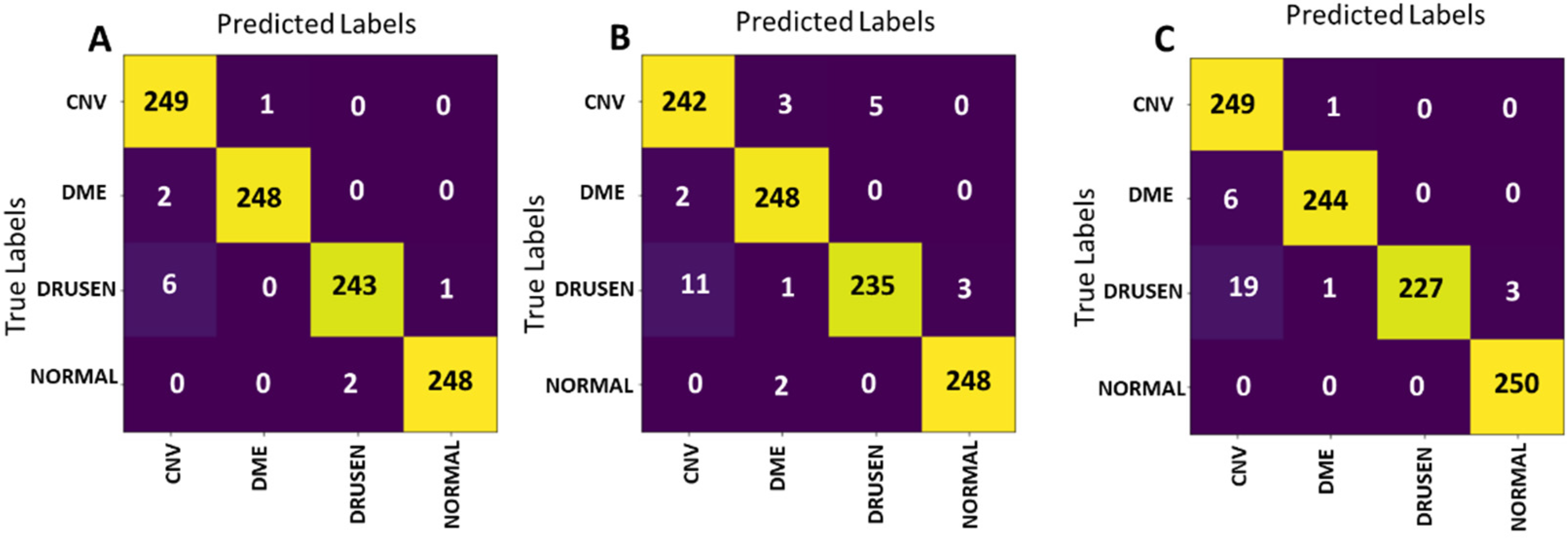
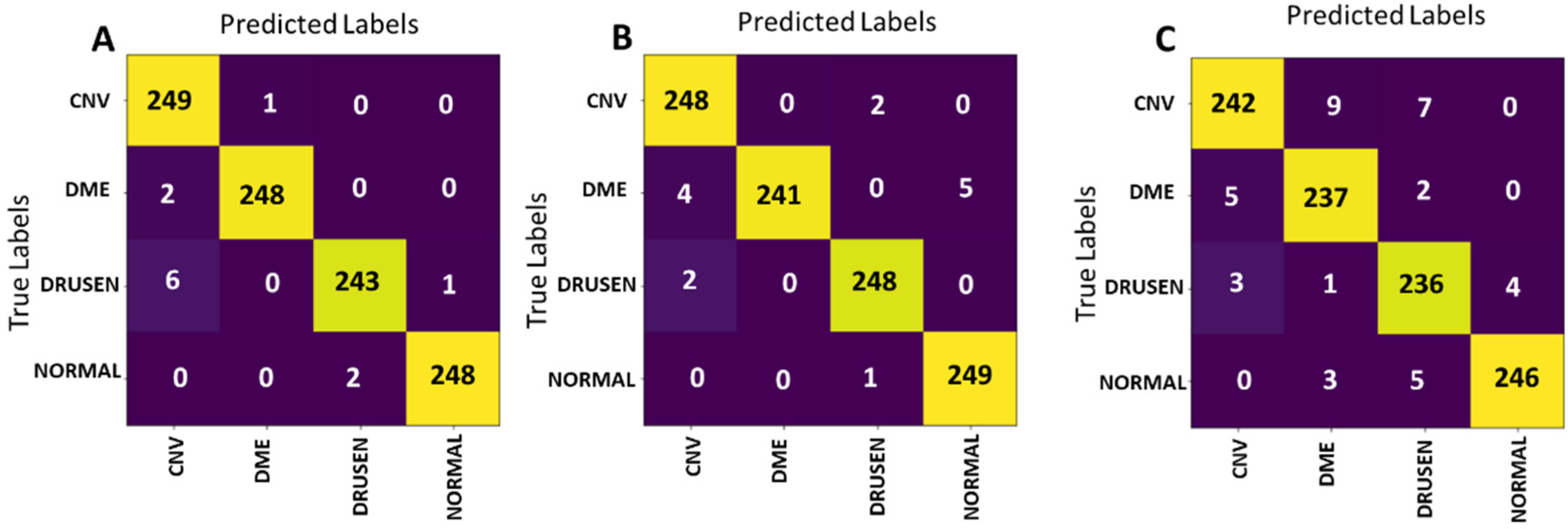
The confusion matrices of the best models of the presented experimental scenarios on the test set are presented in Figure 14. ResNet-50 (Figure 14C) achieves the lowest testing accuracy of 97%. The model’s sensitivity for Urgent referral group is 98.6%, while its specificity is 95.4%. The confusion matrix output by applying the best Norm-VGG16 model on the test set is presented in Figure 14B. The confusion matrix illustrates that 973 out of 1000 testing images were correctly classified. The model’s sensitivity for the Urgent referral group is 98%, while its specificity is 96.6%.

The performance of the models is summarized and compared in

Table 4. Comparison between different architectures.

Model	Accuracy	Sensitivity (UR) (Recall)	Specificity (UR)
ResNet-50 (kernel regularized)	97%	98.6%	95.4%
Norm-VGG16 (kernel regularized)	97.3%	98%	96.6%
HyCAD architecture	98.8%	99.4%	98.2%

Highest reported results are bolded for clarification.

. From the shown results, it is determined that the best performing model is HyCAD architecture according to its confusion matrix presented in Figure 14A, scoring an accuracy of 98.8%. In Urgent referrals group, the HyCAD architecture only misclassified 3 images out of 500 and achieves a sensitivity of 99.4% as shown in Table 4. In the Nonurgent referrals group, the same model misclassified only 9 images out of 500 images and achieves 98.2%. It is worth mentioning that the Norm-VGG16 architecture without Kernel regularization attained a testing accuracy of 96.7% when trained on the dataset from scratch.

2. HyCAD Performance Compared to Pure CNNs Performance and State of the Art

The accuracy per class is calculated and compared with previous models of Kermany et al. [4] and Li et al. [20] in

Table 5. Accuracy per class comparison between proposed models, Kermany et al. and Li et al. models on Large Dataset of Labeled Optical Coherence Tomography (OCT) v3 [25].

Accuracy/Class Models	Urgent Referrals Group		Nonurgent Referrals Group
	CNV	DME	DRUSEN	NORMAL
Kermany et al. 2018 [4]	94.8%	96.8%	94.4%	98.4%
Li et al. 2019 [20]	96.4%	99.2%	99.2%	99.6%
HyCAD model	99.6%	99.2%	97.2%	99.2%
Norm-VGG16 (kernel regularized)	96.8%	99.2%	94%	99.2%
ResNet-50(kernel regularized)	99.6%	97.6%	90.8%	100%

. The per class accuracy is given by dividing the truly classified image for each class by their total number. It is noticeable from the accuracies in Table 5 that the lowest accuracy scored by HyCAD is of DRUSEN class, which is explainable due to the fact that it has the lowest percentage in the training set. Nevertheless, HyCAD with the fused hand-crafted features managed to surpass its CNN counterpart Norm-VGG16 in separating the DRUSEN minority class with a difference of 3.2%.

As shown in Table 5, the proposed HyCAD model achieves a significant increase in accuracy of CNV, DME, DRUSEN by 4.8%, 2.4%, 2.8%, while it attains similar NORMAL accuracy compared to Kermany et al. [4]. The proposed HyCAD model achieves an increase in accuracies of CNV class by 3.2% compared to Li et al. [20].

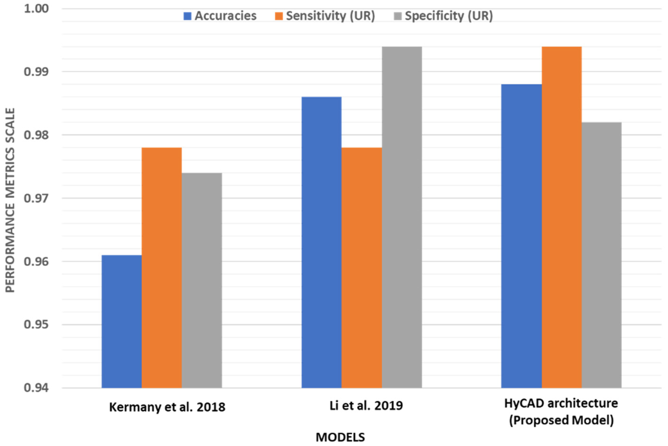
In order to further examine the performance of our best performing model HyCAD architecture relative to the state of the art, its overall performance is compared to the work of Kermany et al. [4] and Li et al. [20]. The comparison is depicted in

Table 6. Comparison between Kermany et al. [4], Li et al. models [20] and HyCAD architecture performance metrics on Large Dataset of Labeled Optical Coherence Tomography (OCT) v3 [25].

Model	Accuracy	Sensitivity (UR)	Specificity (UR)
Kermany et al.2018 [4]	96.1%	97.8%	97.4%
Li et al. 2019 [20]	98.6%	97.8%	99.4%
HyCAD architecture (Proposed model)	98.8%	99.4%	98.2%

Highest reported results are bolded for clarification.

and Figure 15. The values for Kermany et al. [4] and Li et al. [20] are calculated from the best reported confusion matrices as shown in Figure 16. The HyCAD architecture outperforms the work of Kermany et al. [4] in terms of accuracy, sensitivity and specificity scoring an increase of 2.5%, 1.6% and 0.8% respectively. In addition, compared to Li et al. [20], the proposed HyCAD model achieves a noticeable increase in sensitivity by 1.8%, a comparable specificity and a slight increase in accuracy. HyCAD architecture attains the highest sensitivity, scoring an increase of 1.6% compared to the best model of the state of art models [4,20] to reach 99.4% for the Urgent referral group. Such a high sensitivity is required for this group as they represent the critical group, which needs immediate attention. This improvement is achieved while maintaining a competitive specificity with the state of the art.

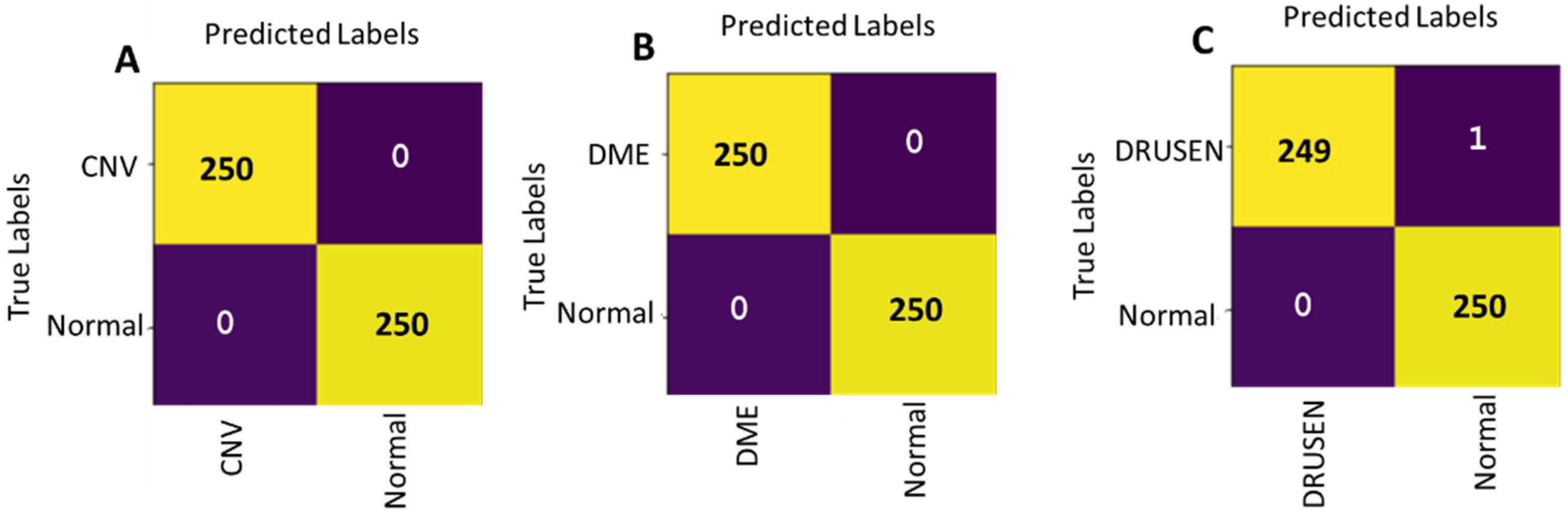
Another important aspect to study is the performance of our HyCAD architecture using hybrid integration of Norm-VGG16 CNN features and hand-crafted features in case of binary classifications. Hence, multiple binary models of CNV vs. NORMAL, DME vs. NORMAL and DRUSEN vs. NORMAL classes are trained and achieve significant results. The respective confusion matrices are shown in Figure 17 and the results are compared to Kermany et al. [4] and Li et al. [20] in

Table 7. Comparison between binary classifiers of HyCAD architecture, Kermany et al. [4] and Li et al. [20] models.

Models	CNV vs. NORMAL			DME vs. NORMAL			DRUSEN vs. NORMAL
	Acc	Sn (CNV)	Sp (CNV)	Acc	Sn (DME)	Sp (DME)	Acc	Sn (DRUSEN)	Sp (DRUSEN)
Kermany et al. 2018 [4]	100%	100%	100%	98.2%	96.8%	99.6%	99%	98%	99.2%
Li et al. 2019 [20]	100%	100%	100%	98.8%	98.8%	98.8%	99.2%	98.4%	100%
HyCAD (Proposed Model)	100%	100%	100%	100%	100%	100%	99.79%	99.6%	100%

Highest reported results are bolded for clarification.

. The two binary models CNV vs. NORMAL vs. DME and NORMAL achieve an accuracy of 100%, sensitivity of 100% and specificity of 100% without any wrong classification of 500 testing set as can be seen from the confusion matrix in Figure 17A,B. The binary model between DRUSEN vs. NORMAL achieves an accuracy of 99.79%, sensitivity of 99.6% and specificity of 100% by classifying only one wrong image as shown in Figure 17C The CNN features are extracted by training Norm-VGG16 for only 15 epochs with learning rate starting with 0.001.

7. Conclusions

In this paper, a novel hybrid computer aided diagnostic system HyCAD-OCT is introduced that effectively distinguishes a range of retinal diseases from OCT scans. The proposed HyCAD architecture integrates deep and traditional learning paradigms to present an accurate timely diagnosis. In addition, HyCAD provides an explainable diagnostic decision through automatic RoI localization using Norm-VGG16 activation maps and the extraction of human articulated features. The automatic RoI localization provides a relative advantage compared to traditional segmentation methods as it does not require expert involvement. Our HyCAD architecture proves the importance of combining automatic feature extraction and hand-crafted features in achieving higher performance metrics. Moreover, the hand-crafted features are more interpretable than the learned features by deep learning architectures models. For the employed deep learning architecture, a set of modifications are applied on the standard VGG16 architecture creating the Norm-VGG16 integrating kernel regularizer variant. Our modified Norm-VGG16 achieved better results than ResNet-50 and Kermany et al. models. HyCAD outperforms the Kermany et al. pure deep learning model in terms of accuracy and Urgent Referrals sensitivity. Similarly, our HyCAD architecture surpassed the Urgent Referrals sensitivity of Li et al. In case of binary classifications of retinal diseases vs. normal, HyCAD had a superior performance compared to both Kermany et al. and Li et al. achieving 100% accuracy, 100% sensitivity and 100% specificity for CNV and DME. For the bootstrapping experiment, HyCAD showed higher mean accuracy and Urgent referrals sensitivity when compared to Norm-VGG16 and ResNet-50. In addition, the results had lower standard deviation. Overall, a new robust diagnostic system is proposed which offers automatic RoI segmentation that can be used in assisting ophthalmologists in their decision with a range of retinal disorders. Moreover, HyCAD is a general architecture that can be trained and applied on similar problems, since no underlying specific assumptions were made that would hinder its generalization.

References

1. Naz, S.; Hassan, T.; Akram, M.U.; Khan, S.A. A practical approach to OCT based classification of Diabetic Macular Edema. In Proceedings of the 2017 International Conference on Signals and Systems (ICSigSys), Bali, Indonesia, 16–18 May 2017; pp. 217–220. [Google Scholar]
2. Hassan, T.; Akram, M.U.; Hassan, B.; Nasim, A.; Bazaz, S.A. Review of OCT and fundus images for detection of Macular Edema. In Proceedings of the 2015 IEEE International Conference on Imaging Systems and Techniques (IST), Macau, China, 16–18 September 2015; pp. 1–4. [Google Scholar]
3. Park, C.; Took, C.C.; Seong, J.-K. Machine learning in biomedical engineering. Biomed. Eng. Lett. 2018, 8, 1–3. [Google Scholar] [CrossRef] [PubMed] [Green Version]
4. Kermany, D.S.; Goldbaum, M.; Cai, W.; Valentim, C.C.S.; Liang, H.; Baxter, S.L.; McKeown, A.; Yang, G.; Wu, X.; Yan, F.; et al. Identifying Medical Diagnoses and Treatable Diseases by Image-Based Deep Learning. Cell 2018, 172, 1122–1131.e1129. [Google Scholar] [CrossRef] [PubMed]
5. Eladawi, N.; Elmogy, M.; Ghazal, M.; Mahmoud, A.H.; Mahmoud, H.; Alhalabi, M.T.; Aboelfetouh, A.; Riad, A.; Keynton, R.; Schaal, S.; et al. 7—Optical coherence tomography: A review. In Diabetes and Fundus OCT; El-Baz, A.S., Suri, J.S., Eds.; Elsevier: Amsterdam, The Netherlands, 2020; pp. 191–221. [Google Scholar] [CrossRef]
6. Vision, E. Macular Edema—What Is It, What Causes it and How Does It Affect Vision? Available online: https://www.enhancedvision.com/low-vision-info/macular-edema-what-is-it-what-causes-it-and-how-does-it-affect-vision.html (accessed on 15 February 2020).
7. Clinic, M. Diabetic Macular Edema. Available online: www.mayoclinic.org/diseases-conditions/diabetic-retinopathy/multimedia/diabetic-macular-edema/img-20124558 (accessed on 12 February 2020).
8. Patel, A.D. Atlas of Clinical Ophthalmology [3rd Edition]. J. Neuro-Ophthalmol. 2006, 26, 237. [Google Scholar] [CrossRef]
9. Cafasso, J. What You Need to Know About Drusen. Available online: https://www.healthline.com/health/drusen (accessed on 15 February 2020).
10. Ghorbel, I.; Rossant, F.; Bloch, I.; Tick, S.; Paques, M. Automated segmentation of macular layers in OCT images and quantitative evaluation of performances. Pattern Recognit. 2011, 44, 1590–1603. [Google Scholar] [CrossRef]
11. Luo, S.; Yang, J.; Gao, Q.; Zhou, S.; Zhan, C.A. The Edge Detectors Suitable for Retinal OCT Image Segmentation. J. Healthc. Eng. 2017, 2017, 3978410. [Google Scholar] [CrossRef] [PubMed] [Green Version]
12. Yang, Q.; Reisman, C.A.; Wang, Z.; Fukuma, Y.; Hangai, M.; Yoshimura, N.; Tomidokoro, A.; Araie, M.; Raza, A.S.; Hood, D.C.; et al. Automated layer segmentation of macular OCT images using dual-scale gradient information. Opt. Express 2010, 18, 21293–21307. [Google Scholar] [CrossRef] [Green Version]
13. Lu, S.; Cheung, C.Y.; Liu, J.; Lim, J.H.; Leung, C.K.; Wong, T.Y. Automated Layer Segmentation of Optical Coherence Tomography Images. IEEE Trans. Biomed. Eng. 2010, 57, 2605–2608. [Google Scholar] [CrossRef]
14. Bagci, A.M.; Rashid, A.; Mahnaz, S. A method for detection of retinal layers by optical coherence tomography image segmentation. In Proceedings of the 2007 IEEE/NIH Life Science Systems and Applications Workshop, Bethesda, MD, USA, 8–9 November 2007; pp. 144–147. [Google Scholar]
15. Niu, S.; Chen, Q.; de Sisternes, L.; Rubin, D.L.; Zhang, W.; Liu, Q. Automated retinal layers segmentation in SD-OCT images using dual-gradient and spatial correlation smoothness constraint. Comput. Biol. Med. 2014, 54, 116–128. [Google Scholar] [CrossRef]
16. Salarian, M.; Ansari, R.; Wanek, J.; Shahidi, M. Acuurate segmentation of retina nerve fiber layer in OCT images. In Proceedings of the 2015 IEEE International Conference on Electro/Information Technology (EIT), Dekalb, IL, USA, 21–23 May 2015; pp. 653–656. [Google Scholar]
17. Garvin, M.; Abramoff, M.; Kardon, R.; Russell, S.; Wu, X.; Sonka, M. Intraretinal Layer Segmentation of Macular Optical Coherence Tomography Images Using Optimal 3-D Graph Search. IEEE Trans. Med. Imaging 2008, 27, 1495–1505. [Google Scholar] [CrossRef] [PubMed]
18. Srinivasan, P.P.; Kim, L.A.; Mettu, P.S.; Cousins, S.W.; Comer, G.M.; Izatt, J.A.; Farsiu, S. Fully automated detection of diabetic macular edema and dry age-related macular degeneration from optical coherence tomography images. Biomed. Opt. Express 2014, 5, 3568–3577. [Google Scholar] [CrossRef] [Green Version]
19. Alsaih, K.; Lemaître, G.; Rastgoo, M.; Massich, J.; Sidibé, D.; Meriaudeau, F. Machine learning techniques for diabetic macular edema (DME) classification on SD-OCT images. BioMed. Eng. OnLine 2017, 16. [Google Scholar] [CrossRef] [PubMed] [Green Version]
20. Li, F.; Chen, H.; Liu, Z.; Zhang, X.; Wu, Z. Fully automated detection of retinal disorders by image-based deep learning. Graefe’s Arch. Clin. Exp. Ophthalmol. 2019, 257, 495–505. [Google Scholar] [CrossRef] [PubMed]
21. Tianyu, Z.; Zhenjiang, M.; Jianhu, Z. Combining CNN with Hand-Crafted Features for Image Classification. In Proceedings of the 2018 14th IEEE International Conference on Signal Processing (ICSP), Beijing, China, 12–16 August 2018; pp. 554–557. [Google Scholar] [CrossRef]
22. Awais, M.; Müller, H.; Tang, T.B.; Meriaudeau, F. Classification of SD-OCT images using a Deep learning approach. In Proceedings of the 2017 IEEE International Conference on Signal and Image Processing Applications (ICSIPA), Kuching, Malaysia, 12–14 September 2017; pp. 489–492. [Google Scholar]
23. Perdomo, O.; Otálora, S.; González, F.A.; Meriaudeau, F.; Müller, H. OCT-NET: A convolutional network for automatic classification of normal and diabetic macular edema using sd-oct volumes. In Proceedings of the 2018 IEEE 15th International Symposium on Biomedical Imaging (ISBI 2018), Washington, DC, USA, 4–7 April 2018; pp. 1423–1426. [Google Scholar]
24. Motozawa, N.; An, G.; Takagi, S.; Kitahata, S.; Mandai, M.; Hirami, Y.; Yokota, H.; Akiba, M.; Tsujikawa, A.; Takahashi, M.; et al. Optical Coherence Tomography-Based Deep-Learning Models for Classifying Normal and Age-Related Macular Degeneration and Exudative and Non-Exudative Age-Related Macular Degeneration Changes. Ophthalmol. Therapy 2019, 8, 527–539. [Google Scholar] [CrossRef] [PubMed] [Green Version]
25. Goldbaum, D.K.a.K.Z.a.M. Large Dataset of Labeled Optical Coherence Tomography (OCT) and Chest X-Ray Images v3. Available online: https://data.mendeley.com/datasets/rscbjbr9sj/3 (accessed on 2 December 2019).
26. Abdellatef, E.; Omran, E.M.; Soliman, R.F.; Ismail, N.A.; Abd Elrahman, S.E.S.E.; Ismail, K.N.; Rihan, M.; Abd El-Samie, F.E.; Eisa, A.A. Fusion of deep-learned and hand-crafted features for cancelable recognition systems. Soft Comput. 2020. [Google Scholar] [CrossRef]
27. Wang, F.; Zhang, C.; Chen, S.; Ying, G.; Lv, J. Engineering Hand-designed and Deeply-learned features for person Re-identification. Pattern Recognit. Lett. 2020, 130, 293–298. [Google Scholar] [CrossRef]
28. Georgiou, T.; Liu, Y.; Chen, W.; Lew, M. A survey of traditional and deep learning-based feature descriptors for high dimensional data in computer vision. Int. J. Multimed. Inf. Retr. 2019. [Google Scholar] [CrossRef] [Green Version]
29. Zhang, H.; Han, H.; Cui, J.; Shan, S.; Chen, X. RGB-D Face Recognition via Deep Complementary and Common Feature Learning. In Proceedings of the 2018 13th IEEE International Conference on Automatic Face & Gesture Recognition (FG 2018), Xi’an, China, 15–19 May 2018; pp. 8–15. [Google Scholar]
30. Xie, Y.; Xia, Y.; Zhang, J.; Feng, D.D.F.; Fulham, M.; Cai, W. Transferable Multi-model Ensemble for Benign-Malignant Lung Nodule Classification on Chest CT. Lect. Notes Comput. Sci. 2017, 10435, 656–664. [Google Scholar] [CrossRef] [Green Version]
31. Buades, A.; Coll, B.; Morel, J. A non-local algorithm for image denoising. In Proceedings of the 2005 IEEE Computer Society Conference on Computer Vision and Pattern Recognition (CVPR’05), San Diego, CA, USA, 20–25 June 2005; Volume 62, pp. 60–65. [Google Scholar]
32. Zisserman, K.S.A.A. Very Deep Convolutional Networks for Large-Scale Image Recognition. arXiv 2014, arXiv:1409.1556. [Google Scholar]
33. Krizhevsky, A.; Sutskever, I.; Hinton, G.E. ImageNet classification with deep convolutional neural networks. Commun. ACM 2017, 60, 84–90. [Google Scholar] [CrossRef]
34. Patterson, J.; Gibson, A. Deep Learning: A Practitioner’s Approach; O’Reilly Media, Inc.: Newton, MA, USA, 2017. [Google Scholar]
35. Chris. What Are L1, L2 and Elastic Net Regularization in Neural Networks? Available online: https://www.machinecurve.com/index.php/2020/01/21/what-are-l1-l2-and-elastic-net-regularization-in-neural-networks/ (accessed on 15 April 2020).
36. Goodfellow, I.; Bengio, Y.; Courville, A. Deep Learning; The MIT Press: Cambridge, MA, USA, 2016. [Google Scholar]
37. Selvaraju, R.R.; Cogswell, M.; Das, A.; Vedantam, R.; Parikh, D.; Batra, D. Grad-CAM: Visual Explanations from Deep Networks via Gradient-Based Localization. Int. J. Comput. Vis. 2020, 128, 336–359. [Google Scholar] [CrossRef] [Green Version]
38. Davies, E.R. Computer and Machine Vision, Fourth Edition: Theory, Algorithms, Practicalities, 4th ed.; Academic Press Inc.: Cambridge, MA, USA, 2012. [Google Scholar]
39. Sonka, M.; Hlavac, V.; Boyle, R. Image Processing, Analysis, and Machine Vision; Thomson-Engineering: Cinderford, UK, 2007. [Google Scholar]
40. Vocal. Histogram of Oriented Gradients (HOG) for Object Detection. Available online: https://www.vocal.com/video/histogram-of-oriented-gradients-hog-for-object-detection/ (accessed on 22 April 2020).
41. Dalal, N.; Triggs, B. Histograms of oriented gradients for human detection. In Proceedings of the 2005 IEEE Computer Society Conference on Computer Vision and Pattern Recognition (CVPR’05), San Diego, CA, USA, 20–25 June 2005; Volume 881, pp. 886–893. [Google Scholar]
42. Tola, E.; Lepetit, V.; Fua, P. A fast local descriptor for dense matching. Proc. CVPR 2008. [Google Scholar] [CrossRef] [Green Version]
43. Hasan, M.; Islam, M.M.; Zarif, M.I.I.; Hashem, M.M.A. Attack and anomaly detection in IoT sensors in IoT sites using machine learning approaches. Internet Things 2019, 7, 100059. [Google Scholar] [CrossRef]
44. He, K.; Zhang, X.; Ren, S.; Sun, J. Deep Residual Learning for Image Recognition. In Proceedings of the 2016 IEEE Conference on Computer Vision and Pattern Recognition (CVPR), Las Vegas, NV, USA, 27–30 June 2016. [Google Scholar] [CrossRef] [Green Version]
45. Rezende, E.; Ruppert, G.; Theophilo, A.; Carvalho, T. Exposing Computer Generated Images by Using Deep Convolutional Neural Networks. Signal Process. Image Commun. 2017. [Google Scholar] [CrossRef] [Green Version]
Figure 1. Illustration of abnormal class vs. normal class (a) CNV vs. NORMAL (b) DME vs. NORMAL (c) DRUSEN vs. NORMAL.
Applsci 10 04716 g001
Figure 2. Dataset classes (CNV, DME, DRUSEN and NORMAL).
Applsci 10 04716 g002
Figure 3. Noised vs. Denoised Images (a) CNV class (b) DME class (c) DRUSEN class (d) NORMAL class.
Applsci 10 04716 g003
Figure 4. The proposed HyCAD system architecture.
Applsci 10 04716 g004
Figure 5. Norm-VGG16: modified VGG16 architecture (in the blocks modification in the VGG16, a block of 2 convolutional neural networks is highlighted followed by batch normalization with feature map 256, max pooling layer and dropout layer added after the block of 128 feature map and maxpooling layer. In addition, At the end of Network a Convolution layer of 512 feature map is added. The dense layer is modified to have a kernel regularizer).
Applsci 10 04716 g005
Figure 6. Grad-CAM overview.
Applsci 10 04716 g006
Figure 7. Examples of heat maps for each class.
Applsci 10 04716 g007
Figure 8. Pipeline of segmentation. (a) CNV class (b) DME class (c) DRUSEN class (d) NORMAL class.
Applsci 10 04716 g008
Figure 9. Mask Generation from heat map (generated from Norm-VGG16 (kernel regularized)).
Applsci 10 04716 g009
Figure 10. Histogram of Oriented Gradients (HOG) descriptor pipeline.
Applsci 10 04716 g010
Figure 11. Neural Network Architecture.
Applsci 10 04716 g011
Figure 12. Confusion matrix.
Applsci 10 04716 g012
Figure 13. Training and Testing Curves for Norm-VGG16 (kernel regularized) and ResNet-50 (kernel regularized) (A) Training accuracy curves (B) Testing accuracy curve (C) Training loss curves (D) Testing loss curve.
Applsci 10 04716 g013
Figure 14. Confusion matrix (A) HyCAD confusion matrix (B) Norm-VGG16 (kernel regularized) (C) ResNet-50 (kernel regularized).
Applsci 10 04716 g014
Figure 15. Comparison between Kermany et al. [4], Li et al. models [20] and HyCAD architecture performance metrics.
Applsci 10 04716 g015
Figure 16. (A) HyCAD architecture Confusion Matrix (B) Li et al. model [20] Confusion Matrix (C) Kermany et al. [4] Confusion Matrix.
Applsci 10 04716 g016
Figure 17. HyCAD architecture binary classifier (A) CNV vs. NORMAL (B) DME vs. NORMAL (C) DRUSEN vs. NORMAL.
Applsci 10 04716 g017