Research on 2D Laser Automatic Navigation Control for Standardized Orchard

Abstract

With the increase of labor cost and the development of agricultural mechanization, standardized orchards suitable for autonomous operations of agricultural machinery will be a future development trend of the fruit-planting industry. For field-planting processes of standardized orchards, autonomous navigation of orchard vehicles in complex environments is the foundation of mechanized and intelligent field operations. In order to realize autonomous driving and path-tracking of vehicles in complex standardized orchards that involve much noise and interference between rows of fruit trees, an automatic navigation system was designed for orchard vehicles, based on 2D lasers. First, considering the agronomic requirements for orchard planting such as plant spacing, row spacing and trunk diameter, different filtering thresholds were established to eliminate discrete points of 2D laser point cloud data effectively. Euclidean clustering algorithm and the important geometric theorems of three points collinearity was used to extract the central feature points of the trunk, as the same time, navigation path was fitted based on the least square method. Secondly, an automatic navigation control algorithm was designed, and the fuzzy control was used to realize the dynamic adjustment of the apparent distance of the pure pursuit model. Finally, the reliability of the proposed approach was verified by simulation using MATLAB/Simulink, and field tests were carried out based on electric agricultural vehicle. Experimental results show that the method proposed in this study can effectively improve the precision of automatic navigation in complex orchard environment and realize the autonomous operation of orchard vehicles.

1. Introduction

In recent years, with the acceleration of the industrialization process and the aging of the population, the problem of insufficient agricultural labor will become increasingly serious. Fruit is an important source of human nutrition and a pillar industry of the planting industry. However, compared with the traditional agriculture, the management technology and the mechanization are relatively backward [1]. In addition, traditional agricultural operations are generally carried out by people or people operating agricultural machinery, and the labor is repeated and monotonous. It is easy for the operator to fatigue, which will cause the operator’s operation accuracy to decrease and the danger to rise for a long time. The modern agricultural equipment led by agricultural robots developed later can largely solve the above problems. Therefore, the system design of this project is suitable for advanced equipment for orchard operations [2,3].

The automatic navigation technology designed by the project senses the surrounding environment through the navigation system, and then the system can assist the robot to complete different tasks. This experiment is an important part of the development of advanced agricultural machinery equipment [4,5,6]. In the early research, many scholars focused on the physical navigation system based on physical orbit [7] and ultrasonic sensor [8], but the systems are susceptible to external environment interference and the labor is not completely liberated. With the continuous development of environment-aware location technology, GNSS navigation has gradually become a research hot-spot [9,10,11]. It demonstrates superiority and great potential in empty environment. However, in the orchard environment, the canopy and branches of the fruit trees are dense, and the GNSS system cannot receive satellite signals stably due to the shadowing, so the applicability is poor.

The difficulty of this experiment lies in the machine vision navigation technology, which is a comprehensive technology based on digital image processing, which has the advantages of great flexibility and rich information acquisition. At present, the types of visual sensors commonly used are mainly monocular cameras and binocular cameras. Monocular cameras are simple in structure and can be used for navigation path extraction in certain types of known environments [12,13], but only two-dimensional information is available due to structural limitations. As early as 1995, Matthies [14] first proved the feasibility of binocular vision technology for unmanned ground vehicles. In recent years, binocular vision technology has also been widely used in agriculture [15,16,17]. However, machine vision hardware is complex in structure, expensive and requires high performance on the processor. At the same time, image information is easily lost due to environmental noise, which affects the accuracy of the guidance system.

Compared with visual navigation, laser navigation has many advantages such as high range accuracy and strong anti-interference ability. Laser navigation technology, according to different structures, can be divided into 2D laser and 3D laser. The 3D laser realizes environmental mapping in three-dimensional space by multi-line mixing (combining 2D laser or monocular vision) [18,19,20] or solid-state rotation (adding pan tilt scanning device) [21,22,23,24]. Two-dimensional lasers typically use only one set of laser sensors to scan on one line. Oscar of Hokkaido University and Chen of Northwest A&F University [25,26,27] designed a 2D laser automatic navigation system suitable for orchard environment and verified the reliability of the system with a small horsepower tractor as an experimental platform. After research, it was found that the lateral error in navigation was 11 cm and the heading angle error was 1.5°. Pawin [28] of Tsukuba University in Japan used 2D lasers and Kubota Kingwel tractors as an experimental platform. The researchers at the university designed an automatic curve navigation driving system for orchards. The experiment showed that the average deviation of path-tracking was 0.275 m. The standard deviation is 0.009 mm. Gokhan [29] considered the wheel slip and used the cheap 2D laser to realize the straight walking and ground turning of the tractor in the apple orchard.

Environmental awareness is an important part of the navigation system. In laser positioning system, positioning accuracy and quality depend on many factors such as the laser incidence angle [30], scanning object geometry [31] and object surface characteristics [32,33]. In order to improve the positioning accuracy and quality, different algorithm models were used to complete the noise reduction processing with different recognition of the surface features of objects. For the sphere, Urbančič [34] provided two methods of parameter acquisition and verified the accuracy and effectiveness of the algorithm. In this paper, the standardized apple orchard with good consistency of row spacing parameters were the research environment. The trunks are relatively smooth and complete which can be viewed as cylinder approximately. Considering the principle of economy, 2D laser will play a huge potential in the application of standardized orchard fruit positioning.

Many scholars have done a lot of research on solving the problem of noise interference in fruit trees [35,36,37], and some progress has been made. However, the existing research of the acquisition and processing of laser point cloud data ignores the influence of obstacles such as weeds and irregular tree trunks. If the necessary filtering is not carried out, it will cause a large deviation in the fitted navigation baseline. Some researchers have been developed path-tracking controller with high accuracy and strong robustness by using Proportion Integration Differentiation (PID) [38], fuzzy control [39] or sliding mode control [40], but due to the lack of positioning accuracy, the navigation control accuracy will be seriously affected.

This paper designed an automatic navigation system for standardized orchards with 2D laser for orchard low-speed operation wheeled vehicles. The system considers the influence of small interfering objects on the traveling route of the wheeled vehicle on the accuracy of the point cloud data acquired by the 2D laser. The distance threshold and the statistical filtering were used to complete the filtering process. Euclidean clustering algorithm and the important geometric theorems of three points collinearity was used to extract the central feature points of the trunk. Finally, the linear navigation path was identified and extracted by the least square method. Based on obtaining lateral deviation and heading deviation, this paper designed an adaptive pure pursuit path-tracking controller combined with the advantages of fuzzy control without the need to construct an accurate mathematical model. The modified agricultural electric vehicle was used as an experimental platform for simulation and field tests in order to verify the accuracy and robustness of the automatic navigation system.

2. Materials and Methods

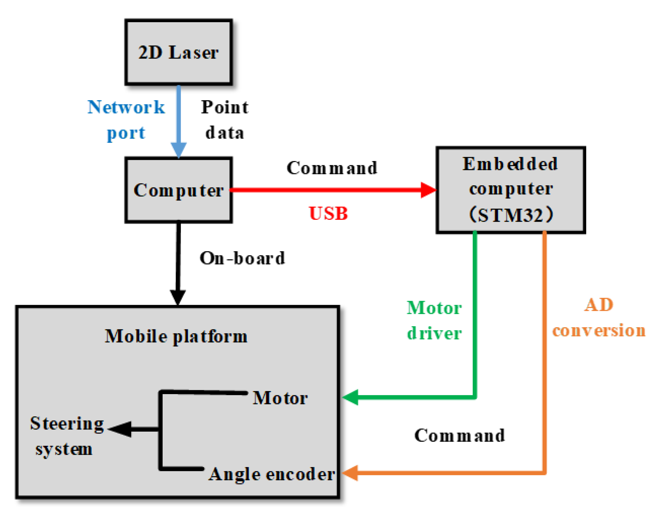
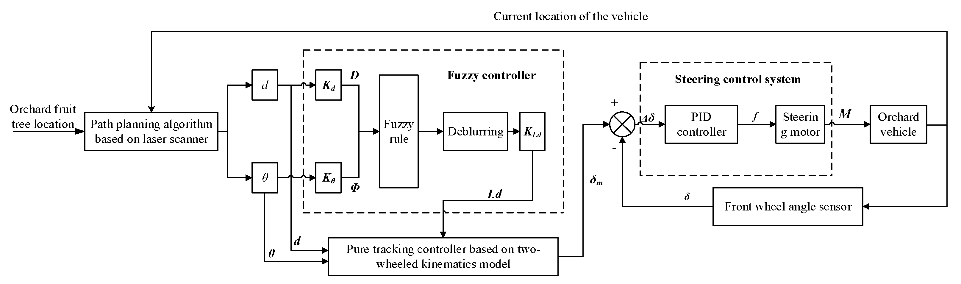
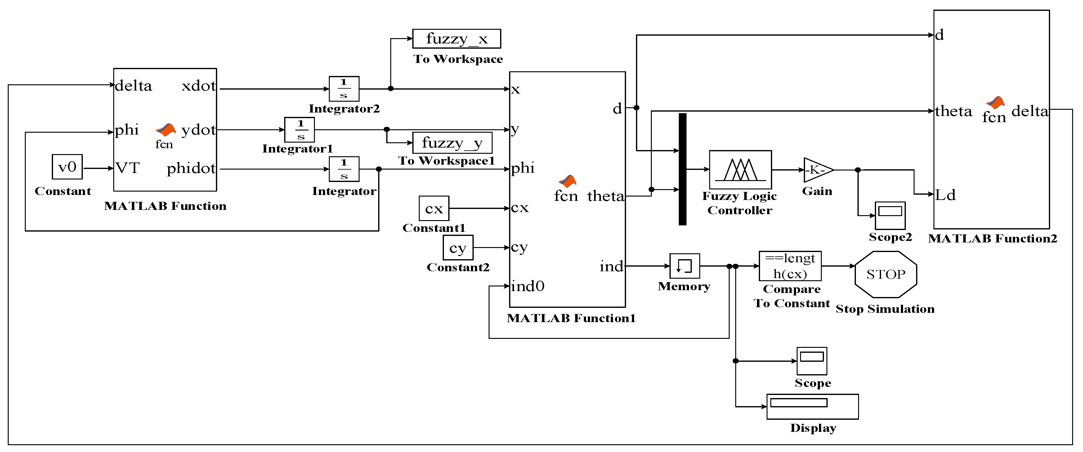
2.1. System Composition

The orchard vehicle automatic test platform based on the electric agricultural vehicle (model: SH-GL) was mainly composed of 2D laser, automatic steering system and front wheel rotation angle detection system. The structure of the test platform is shown in Figure 1. The laser was installed at the center of the front of the vehicle, the height was 0.6 m from the ground and data were transmitted to the main controller PC through the network port. The automatic steering system was composed of 86BYGH2503 stepper motor, DLD6-20B electromagnetic clutch and chain transmission. Based on Stm32F103 which communicates with the main controller PC through the USB serial port, it realizes automatic steering through Proportion Integration Differentiation (PID) control. The front wheel angle system was based on Wittower-RE38 encoder and communicates with the Stm32F103 through AD conversion. A tracking device was fixed at the center axis of the test platform and made the ink outlet of the device as close to the ground as possible. The white ink was placed in the tracking device, and the actual walking path of the test platform was recorded by the ink droplet trajectory.

The 2D laser was UST-20LXLiDAR manufactured by HOYUKO. Its specific parameters are shown in

Table 1. Specifications of the laser range sensor.

Description	Parameter
Light source	Semiconductor laser (905 nm)
Measuring range	0.06 (m)–8 (m) Maximum detection distance 60 (m)
Ranging accuracy	40 (mm)
Angular resolution	0.25°
Maximum scanning range	270°
Scanning period	25 (ms)

. As shown in Figure 2, the navigation control terminal PC was the core of the control system. This study was based on Windows 10 Visual Studio 2015 for data processing and software algorithm design.

In order to test the performance of the front wheel angle system, a bench test was designed. The front wheel was set up, the test platform was in no-load state and the pulse control signal was applied to control the front wheel of the test platform to rotate 30° to the left and right (the maximum rotation angle of the test platform was [−30°, 30°]). The result is shown in Figure 3. The fitting degree R² of the regression equation of the left and right turn response curves of the test platform was 0.9938 and 0.9918, respectively, indicating that the system obtains the rotation angle as linear.

In order to test the performance of the automatic steering control system, the sine wave steering tracking test was designed. Place the test platform on the open concrete pavement, apply a sine wave signal with frequency of 0.5 πHz and an angular amplitude of 10°. Finally, record front wheel angle data. The test results are shown in Figure 4. The electric steering control system can track the control signal well, with slight oscillation near the peak ±10°, the large tracking error was 0.86° and the average absolute tracking error was 0.304°, indicating that the automatic steering control system has better performance.

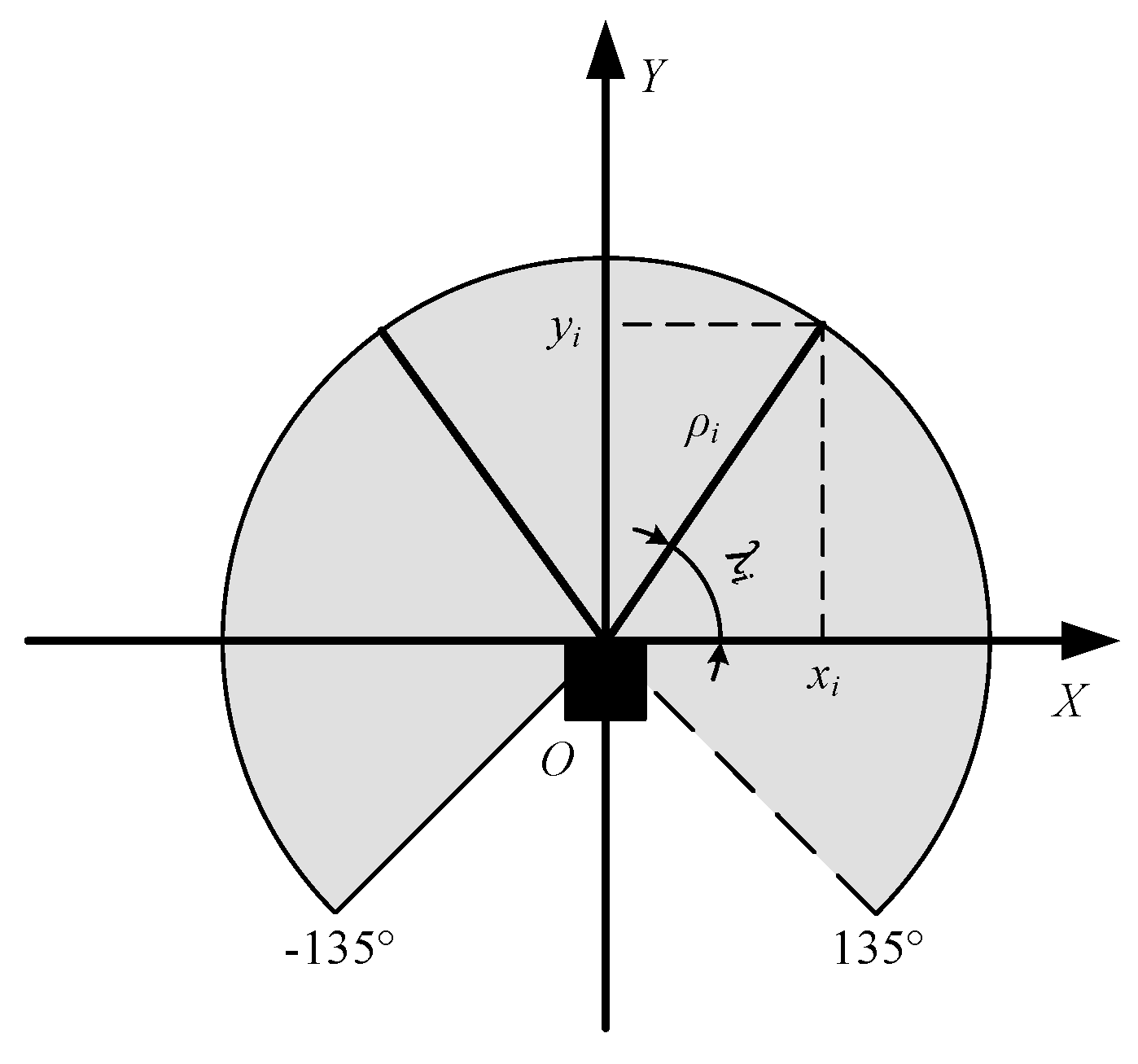
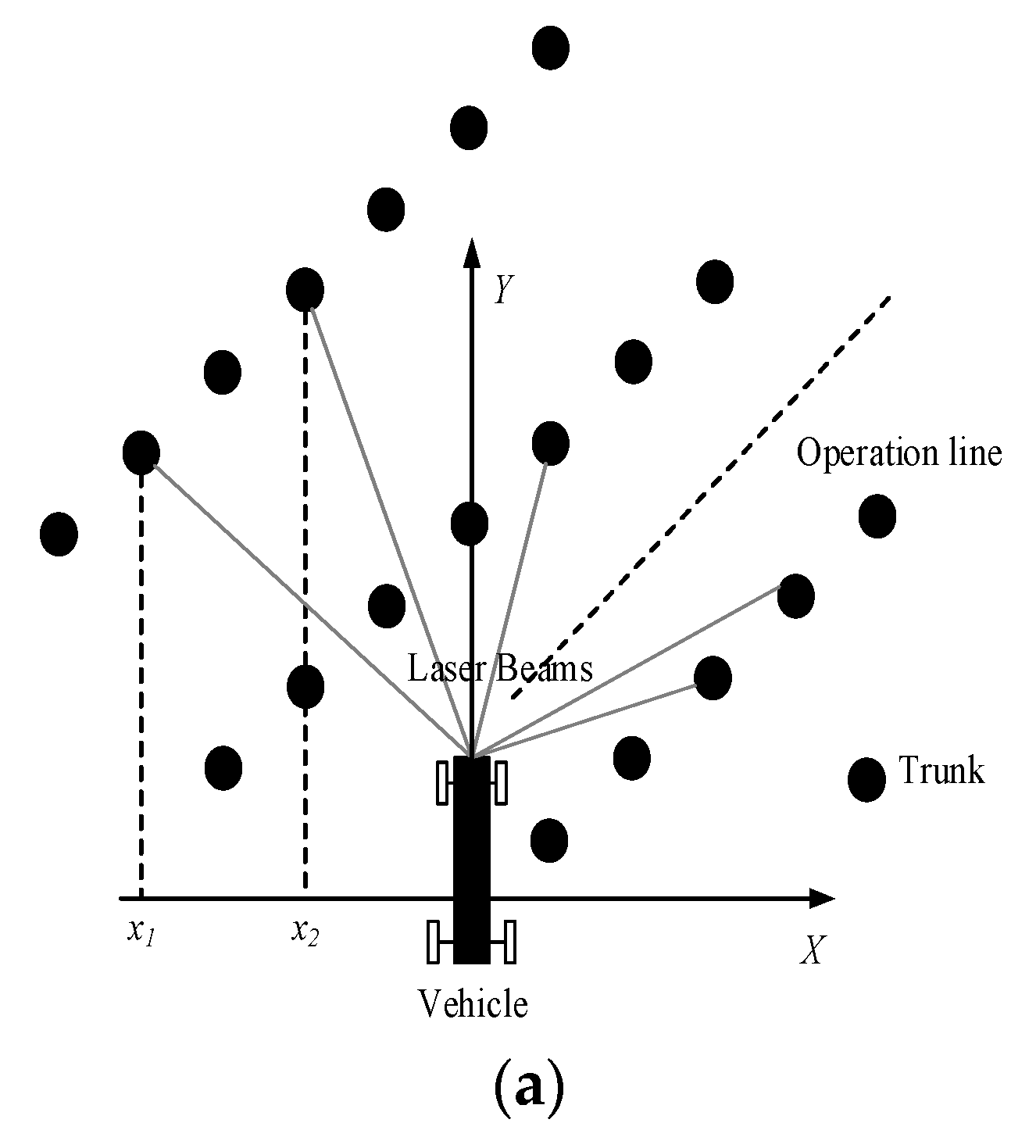
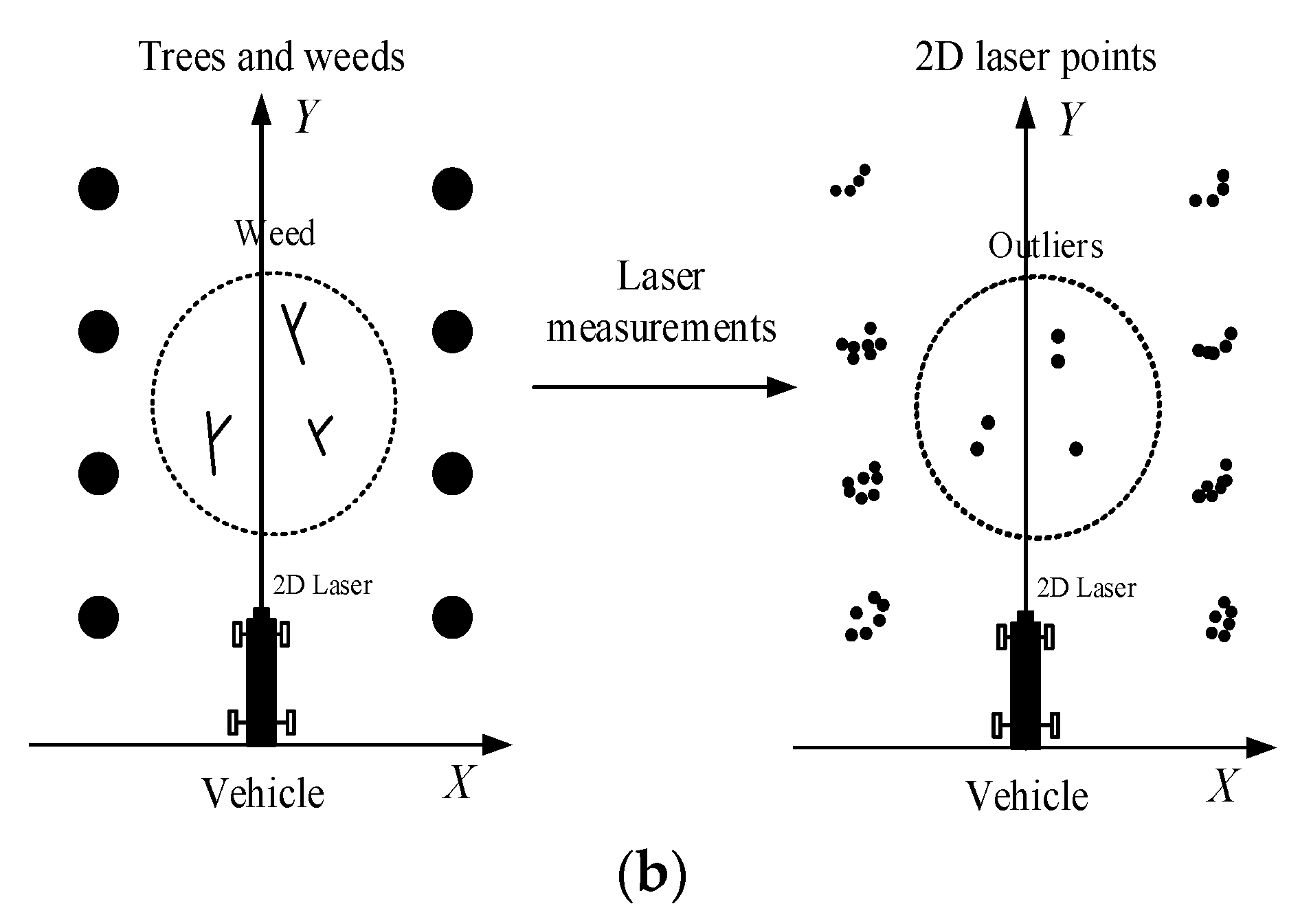
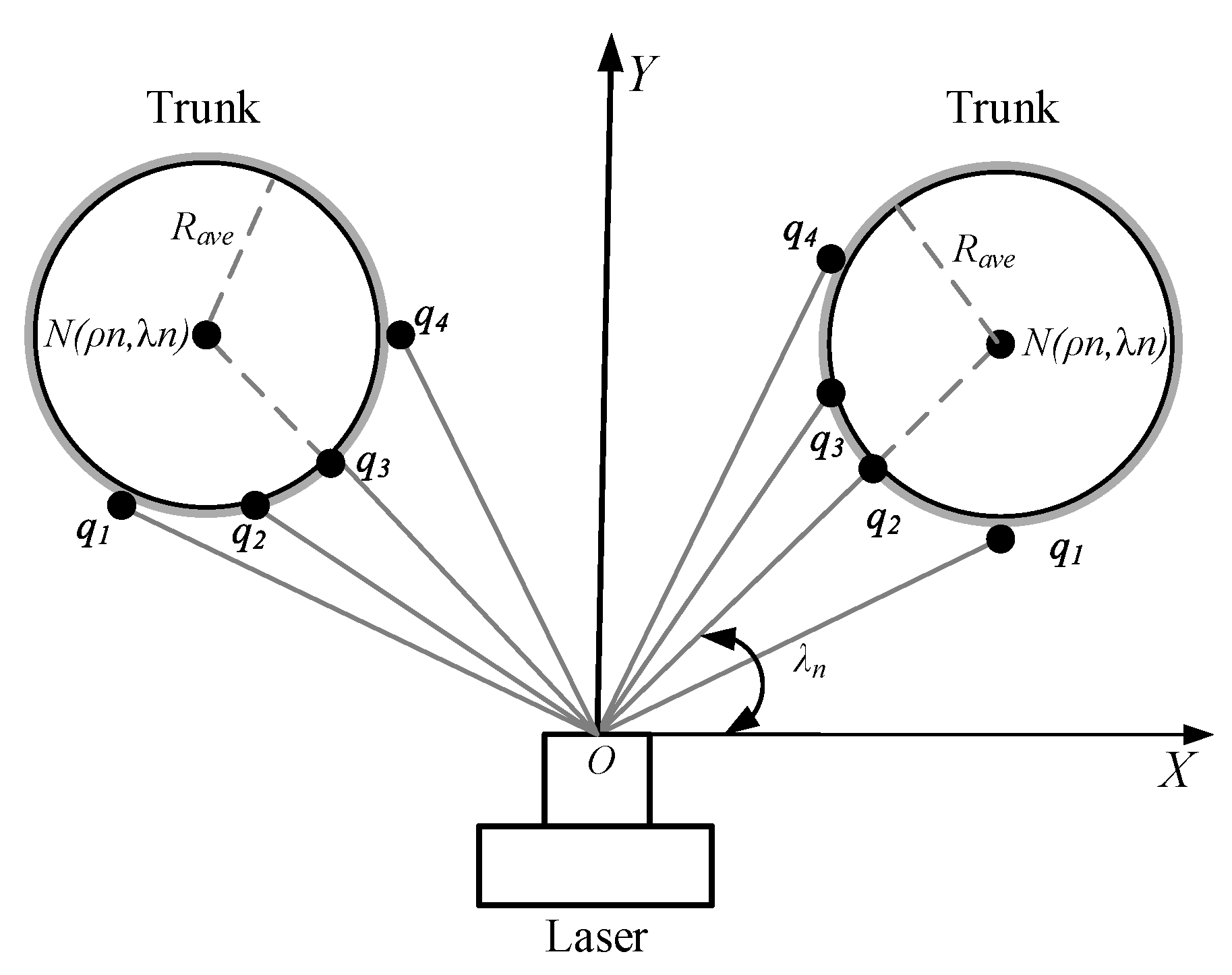
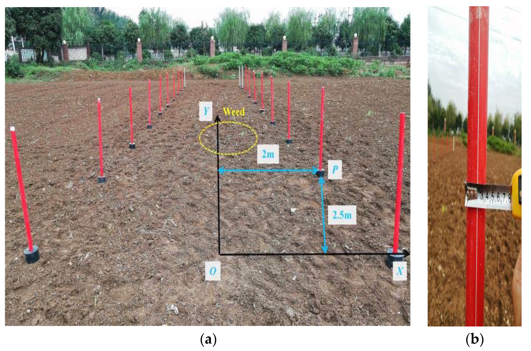
2.2. Fruit Tree Position Information Determination

When using the 2D laser to scan the orchard environment, the laser receiver will receive signal feedback with different lengths due to the occlusion of the laser pulse by the trunk. According to this principle, the position of the fruit tree can be determined.

As shown in Figure 5, we have established a rectangular coordinate system with the laser scanner’s mounting position O as the origin and the Y-axis in the vehicle’s forward direction. The ρ_i is the distance between the laser scanner’s emission point and the target. The λ_i is the angle formed laser beam with the coordinate axis. The point (x_i, y_i) is the Cartesian coordinates of the i-th point scanned by the 2D laser.

By the Equation (1), we complete the process of the Cartesian coordinate transformation of the fruit tree position information.

$$\{\begin{array}{l}{x}_i={\rho }_i\times \cos {\lambda }_i\\ y_i={\rho }_i\times \sin {\lambda }_i\end{array}$$

(1)

Due to the complex environment of the orchard, there were more interference points or outlier noise in the point cloud data acquired by the 2D laser, which seriously affects the accuracy of the navigation path identification. Therefore, the acquired point cloud data needs to be filtered first.

As shown in Figure 6a, when the heading direction of the vehicle differs greatly from the navigation path, the laser beam can obtain the fruit tree information at a long distance through the spacing of the plant spacing between the fruit trees, thereby causing interference to obtain effective information. We set the i-th data point to q_i. Its eigenvector is shown in Equation (2). Set the distance thresholds to ρ_max and x_max. If ρ_i < ρ_max and x_i < x_max, q_i is retained. Otherwise it is eliminated.

$$q_i={[{\rho }_i,{\lambda }_i,x_i,y_i]}^T$$

(2)

When there were small obstacles such as weeds, it does not affect the travel of the vehicle. The laser data of this experiment often contains some discrete points, as shown in Figure 6b. The d_i is the Euclidean distance from point q_i to any point. The D_avr-i is the average distance of q_i to all its k neighbors and the H_i is the standard range of calculation.

$$\{\begin{array}{l}{D}_{avr-i}=\frac{1}{k}{\displaystyle \sum _{i=1}^k{d}_i}\\ H_i=\mu \pm g\times \sigma \end{array}$$

(3)

As shown in the Equation (3), we can see that μ is the distance mean, σ is the distance standard deviation and g is the constant coefficient of standard range H_i. When D_avr-i > H_i, the point is regarded as a discrete point and culled. Otherwise it is retained.

When we obtain the complete fruit tree coordinate points, we use European clustering to cluster all the coordinate points on the same fruit tree. As shown in the equations (4), M_i,i+1 is the Euclidean distance of the laser data points q_i and q_i+1. The cluster search radius is r and its value is related to the average radius of the fruit trees.

$$M_{i,i+1}=\sqrt{{(x_{i+1}-x_i)}^2+{(y_{i+1}-y_i)}^2}$$

(4)

When M_i,i+1 < r, we think that two points come from the same fruit tree and gather into one kind; when M_i,i+1 > r, we think that two points come from different fruit trees.

Through this experiment, we found that the point cloud data region obtained by the 2D laser scanner is the outer surface of the fruit tree trunk at the current laser height. The trunk of the fruit tree can be approximated as a cylinder, and the central feature point of the trunk can be extracted using the important geometric theorem of three points collinearity.

As shown in Figure 7, we set the polar coordinates of the central feature point of the trunk as N(ρ_n, λ_n), the n consecutive data points of the trunk cluster are q_n, the point with the smallest ρ value is selected as the feature point (ρ_min, λ_min) and the R_ave is expressed as the average radius of the fruit tree trunk. The Equation (5) can be obtained through geometric derivation.

$$\{\begin{array}{l}{\lambda }_n={\lambda }_{\min }\\ {\rho }_n={\rho }_{\min }+R_{ave}\end{array}$$

(5)

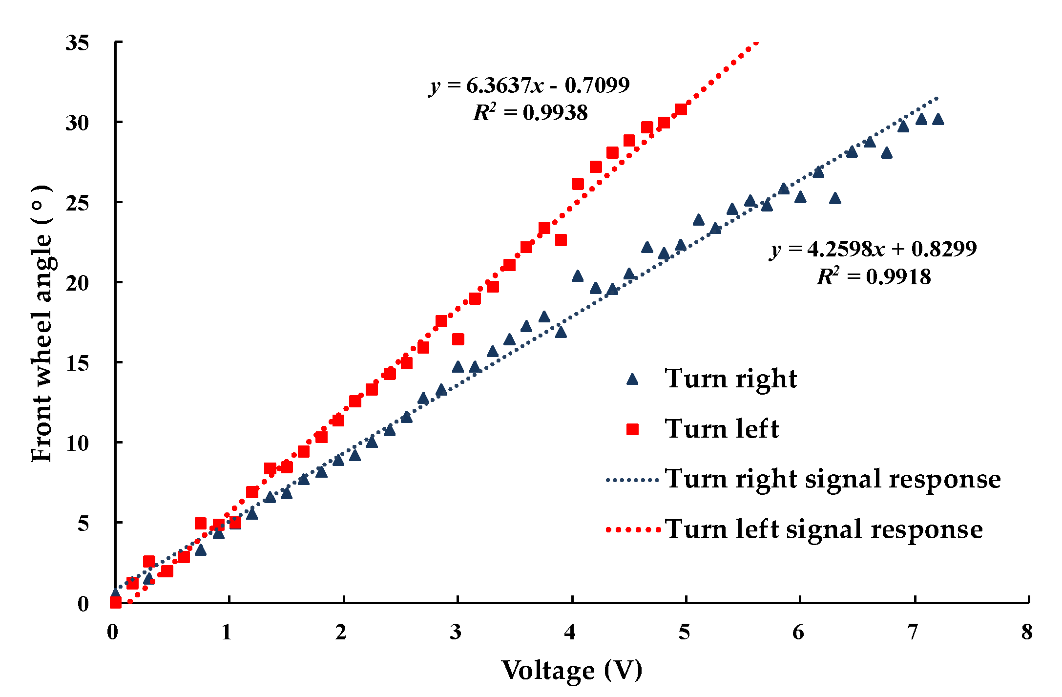
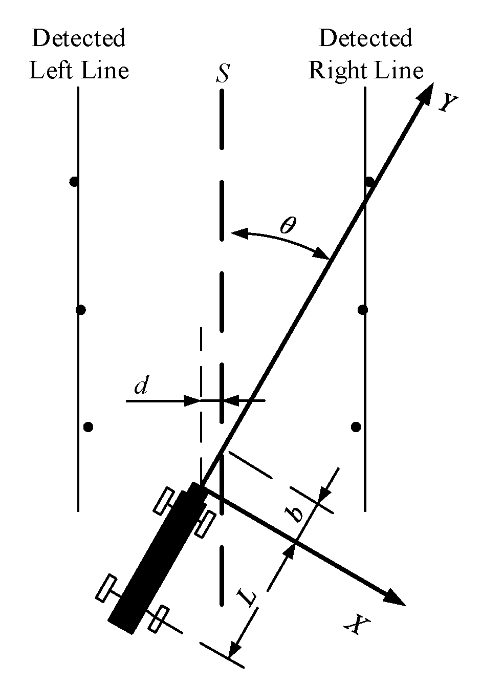
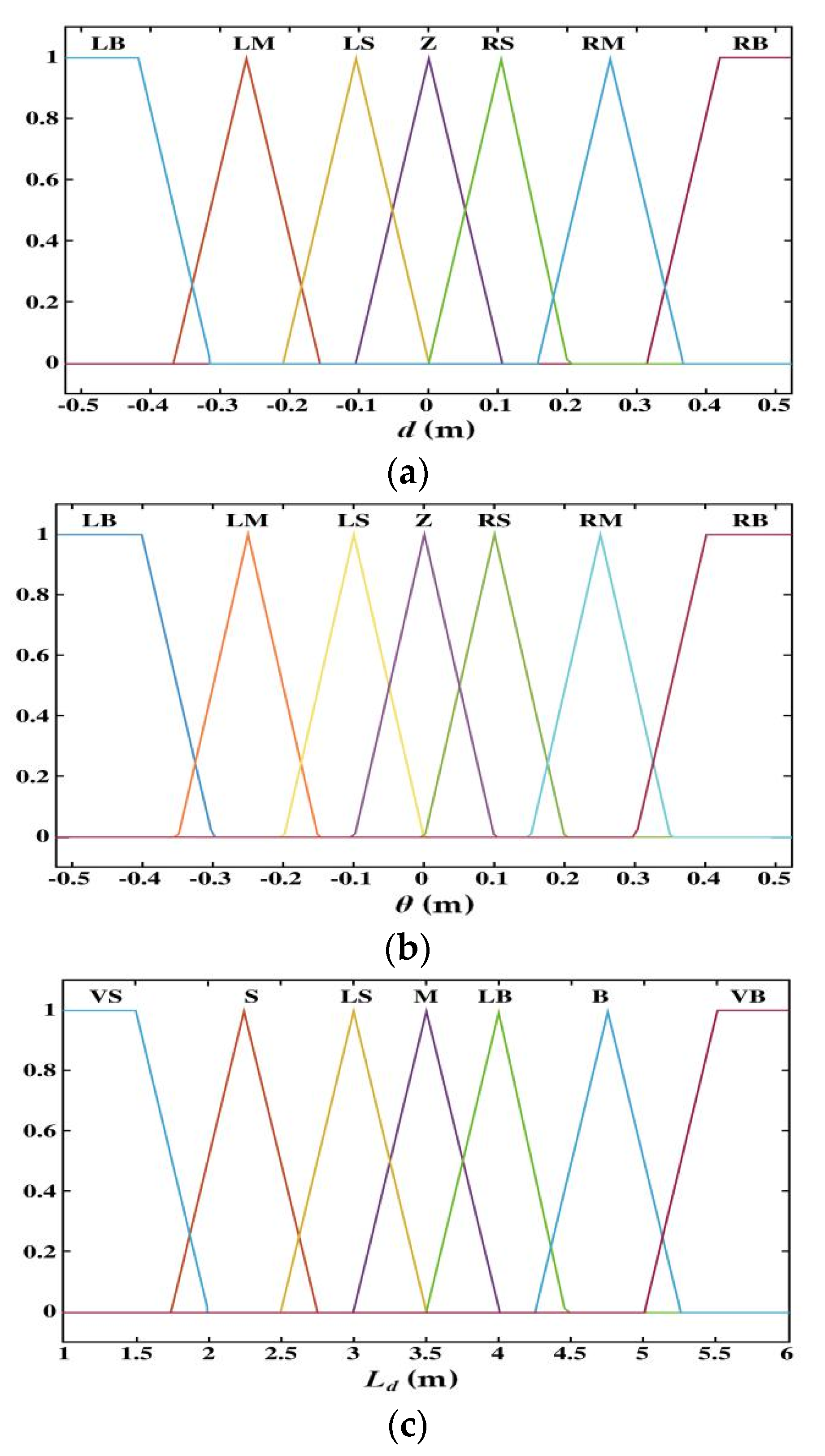
2.3. Navigation Control Parameter Acquisition

In order to obtain the vehicle navigation path, this experiment needs to fit the central feature points of all trunks in a straight line. We set the coordinates of the center points of the left and right fruit trees as (x_li, y_li) and (x_ri, y_ri). In this experiment, the coordinates of the center points of the three fruit trees on the left and right sides of the vehicle are selected to form two groups, forming 9 groups. Use the following equation to find the midpoint coordinates (x_c, y_c).

$$\{\begin{array}{l}{x}_c=\frac{x_{li}+x_{ri}}{2}\\ y_c=\frac{y_{li}+y_{ri}}{2}\end{array}$$

(6)

Set the fitted line to be y = ax + b, where a represents the slope of the fitted line and b represents the intercept with the Y-axis. The best estimate of the parameters a, b is obtained according to the Equation (7):

$$\{\begin{array}{c}a=\frac{9({\displaystyle \sum _{i=1}^c{x}_c{y}_c})-{\displaystyle \sum _{i=1}^c{x}_c{\displaystyle \sum _{i=1}^c{y}_c}}}{9{\displaystyle \sum _{i=1}^c{x}_c^2-({\displaystyle \sum _{i=1}^c{x}_c{)}^2}}}\\ b=\frac{({\displaystyle \sum _{i=1}^c{x}_c^2{y}_c})-{\displaystyle \sum _{i=1}^c{x}_c({\displaystyle \sum _{i=1}^c{x}_c{y}_c})}}{9{\displaystyle \sum _{i=1}^c{x}_c^2-({\displaystyle \sum _{i=1}^c{x}_c{)}^2}}}\end{array}$$

(7)

After completing the navigation path fitting, we need to obtain the navigation parameters for implementing the automatic navigation control of the vehicle according to the current position of the vehicle. As shown in Figure 8, The line S is a navigation path, the angle θ between the line S and the Y-axis is the heading deviation, and the flat distance d between the center position of the laser and the line S is the lateral deviation.

The calculation equation of heading deviation θ and lateral deviation d in this experiment are as follows:

$$\begin{array}{c}\theta =\{\begin{array}{l}(\arctan k+\frac{\pi }{2})\times \frac{180}{\pi },k<0\\ (\frac{\pi }{2}-\arctan k)\times \frac{180}{\pi },k>0\end{array}\\ d=b\times \sin \theta \end{array}$$

(8)

As shown in the Equation (8), k is the slope of the navigation path, and b is the intercept of the navigation path.

2.4. Navigation Controller Design

The navigation controller of this experiment was mainly composed of 2D laser acquisition and processing system, path-tracking control system and automatic steering control system. We collect the fruit tree information in real time from the 2D laser and send it to the main controller PC which processes the acquired laser data. The system recognizes the navigation path and calculates the front wheel angle of the vehicle target and sends it to the Stm32F103. The embedded development platform uses PID control to drive the stepper motor to rotate and adjust the front wheel angle to achieve path-tracking. The working principle of the control system is shown in Figure 9.

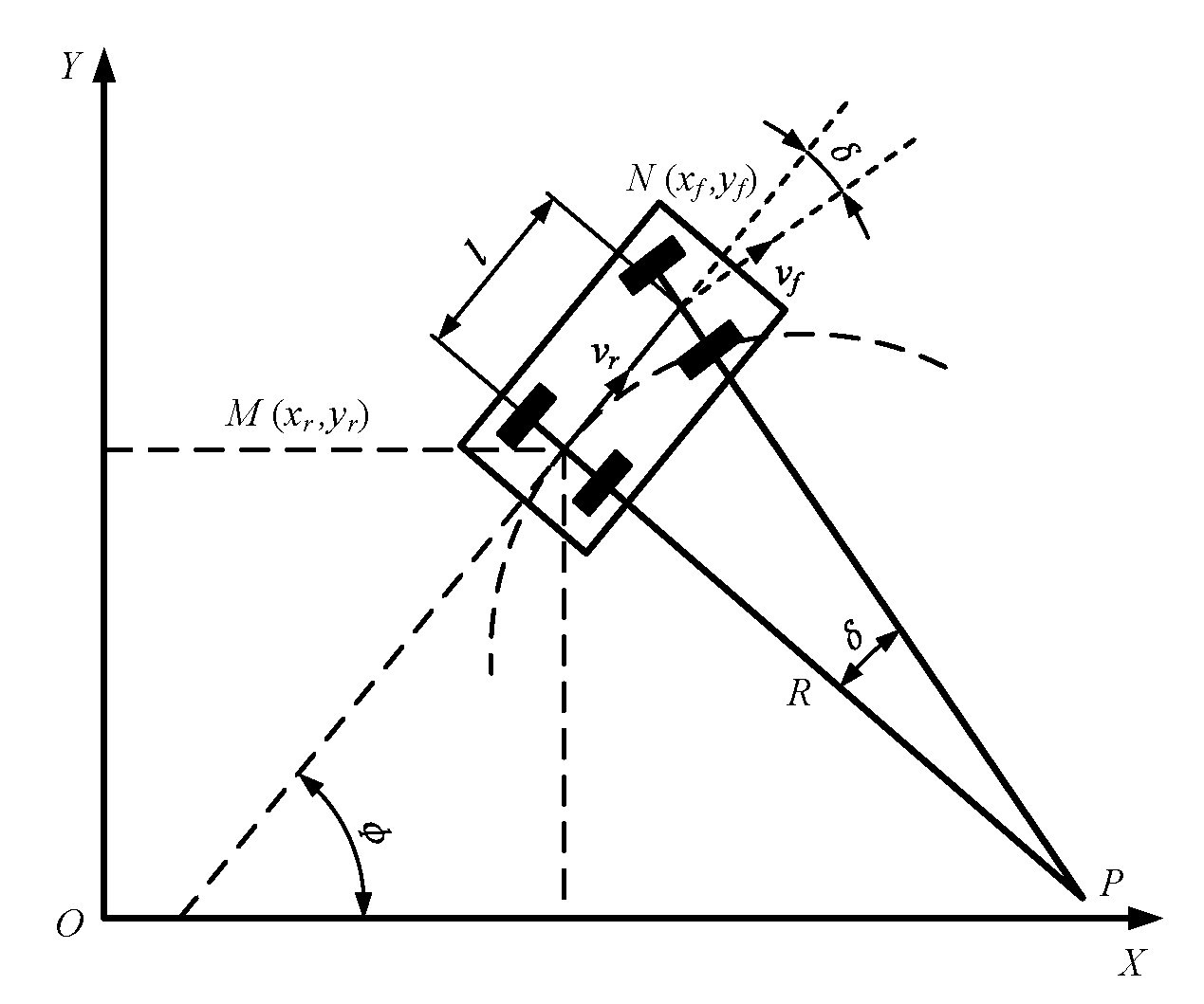
2.4.1. Calculating the Target Front Wheel Angle

Generally speaking, orchard vehicles always complete various operations at low speed. This experiment does not consider the deformation and lateral slip of the tire due to the pressure. The vehicle kinematics model shown in Figure 10 is established.

According to the vehicle kinematics model in Figure 10, the front turning angle of vehicle can be obtained:

$$\delta =\arctan (l/R)$$

(9)

As show in the Figure 11, a pure pursuit model under the line tracking condition is established. According to the geometric relationship in Figure 11, the vehicle’s turning curve γ and the target’s abscissa x_g in the car body coordinate system can be obtained:

$$\gamma =2\frac{x_g}{L_d^2}$$

(10)

$$x_g=d\cos \theta -\sqrt{L_d^2-d^2}\sin \theta$$

(11)

Combined with the above Equations (9)–(11), the front turning angle of vehicle under pure pursuit model can be obtained:

$$\delta =\arctan (\frac{2l(d\cos \theta -\sqrt{L_d^2-d^2}\sin \theta )}{L_d^2})$$

(12)

When the forward-looking distance is selected to be larger, the vehicle will drive along the smaller curvature to the desired path, resulting in a longer control response time [41]. When the forward-looking distance is too small, the system will cause the vehicle to approach the set route along the large arc curve, causing the system to generate large oscillations. Therefore, this paper uses fuzzy controller to adaptively adjust the forward-looking distance in the pure pursuit algorithm to overcome the above shortcomings.

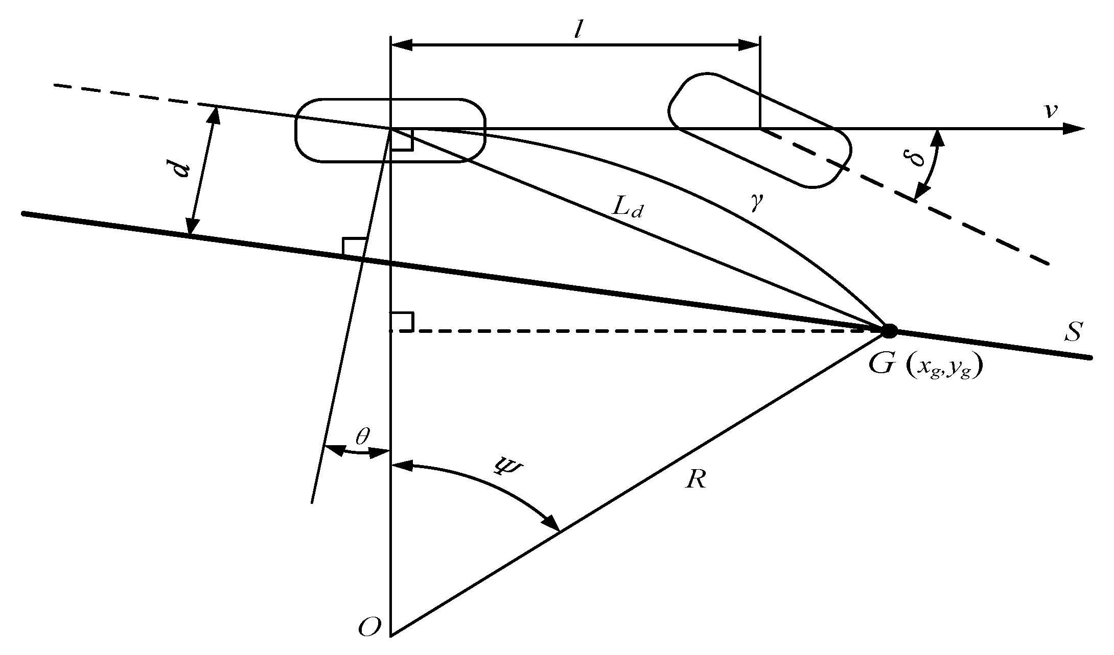
2.4.2. Adaptive Pure Tracking Model Controller Design

After research, we found that the magnitude of the forward-looking distance was affected by both the lateral deviation d and the heading deviation θ. Therefore, d and θ were used as the input of the fuzzy controller and L_d was used as the output. The L_d was adjusted in real time by the fuzzy controller. When d and θ were large, the smaller L_d was used to make the vehicle approach the tracking path quickly, reduce the system adjustment time and improve the system response speed. When d and θ were small, a larger L_d was used to prevent system overshoot and improve system stability.

We set the basic domain of the lateral deviation d to [−0.5 m, 0.5 m] and divide it into 13 levels with quantization levels: {−6, −5, −4, −3, −2, −1, 0, 1, 2, 3, 4, 5, 6}, the corresponding quantization factor K_d = 0.12. The basic domain of the heading deviation θ was [−π/6, π/6], which is divided into 13 levels with quantization levels: {−6, −5, −4, −3, −2, −1, 0, 1, 2, 3, 4, 5, 6}, quantization factor K_θ = 0.087. The basic domain of the forward-looking distance L_d is [1 m, 6 m], which is divided into 6 levels, the quantization levels: {1, 2, 3, 4, 5, 6}, and the quantization factor K_Ld = 1.

According to the positional relationship between the orchard intelligent vehicle and the orchard navigation center line, the lateral deviation d and the heading deviation θ are divided into seven levels: left big (LB), left medium (LM), left small (LS), zero (ZO), right small (RS), right medium (RM), right big (RB). The forward-looking distance L_d is divided into seven levels: very small (VS), small (S), little small (LS), medium (M), little big (LB), big (B), very big (VB). Then, the distribution of this fuzzy variable membership function can be seen in the following Figure 12.

After several anti-simulation experiments, the optimal 49 fuzzy control rules were determined as shown in

Table 2. Fuzzy Control Rule Table.

θ	d
	LB	LM	LS	Z	RS	RM	RB
LB	VS	S	S	VS	S	S	VS
LM	VS	LS	M	LS	M	M	VS
LS	VS	M	LB	LB	LB	M	VS
Z	VS	LB	VB	VB	VB	LB	VS
RS	VS	M	LB	LB	LB	M	VS
RM	VS	LS	M	LS	M	LS	VS
RB	VS	S	S	VS	LS	S	VS

; the fuzzy control surface was plotted as shown in Figure 13.

In this study, Mamdani’s fuzzy reasoning method and extremely small fuzzy logic inference synthesis rules were used; the defuzzification work is completed by the center of gravity method [42]. The fuzzy control query table is shown in

Table 3. Forward looking distance fuzzy control query table.

Ld (m)		d (m)
		−6	−5	−4	−3	−2	−1	0	1	2	3	4	5	6
θ (rad)	−6	1.38	1.38	1.70	2.25	2.25	2.06	1.38	2.06	2.25	2.25	1.70	1.38	1.38
	−5	1.38	1.38	1.70	2.25	2.25	2.06	1.38	2.06	2.25	2.25	1.70	1.38	1.38
	−4	1.43	1.43	1.72	2.27	2.30	2.05	1.46	2.05	2.29	2.28	1.74	1.43	1.43
	−3	1.39	1.39	1.95	3.00	3.34	3.40	3.00	3.40	3.50	3.50	2.12	1.39	1.39
	−2	1.46	1.46	2.34	3.26	3.57	3.57	3.51	3.57	3.76	3.50	2.24	1.46	1.46
	−1	1.39	1.39	2.37	3.58	4.28	4.32	4.31	4.32	4.28	3.58	2.37	1.39	1.39
	0	1.38	1.38	2.28	4.00	5.05	5.61	5.62	5.61	5.05	4.00	2.28	1.38	1.38
	1	1.39	1.39	2.37	3.58	4.28	4.32	4.31	4.32	4.28	3.58	2.37	1.39	1.39
	2	1.46	1.46	2.34	3.26	3.57	3.57	3.51	3.57	3.57	3.26	2.34	1.46	1.46
	3	1.39	1.39	1.95	3.00	3.34	3.40	3.00	3.40	3.34	3.00	1.95	1.39	1.39
	4	1.43	1.43	1.72	2.27	2.30	2.05	1.46	2.54	2.75	2.27	1.72	1.43	1.43
	5	1.38	1.38	1.70	2.25	2.25	2.06	1.38	2.61	2.74	2.25	1.70	1.38	1.38
	6	1.38	1.38	1.70	2.25	2.25	2.06	1.38	2.61	2.74	2.25	1.70	1.38	1.38

.

3. Results and Discussion

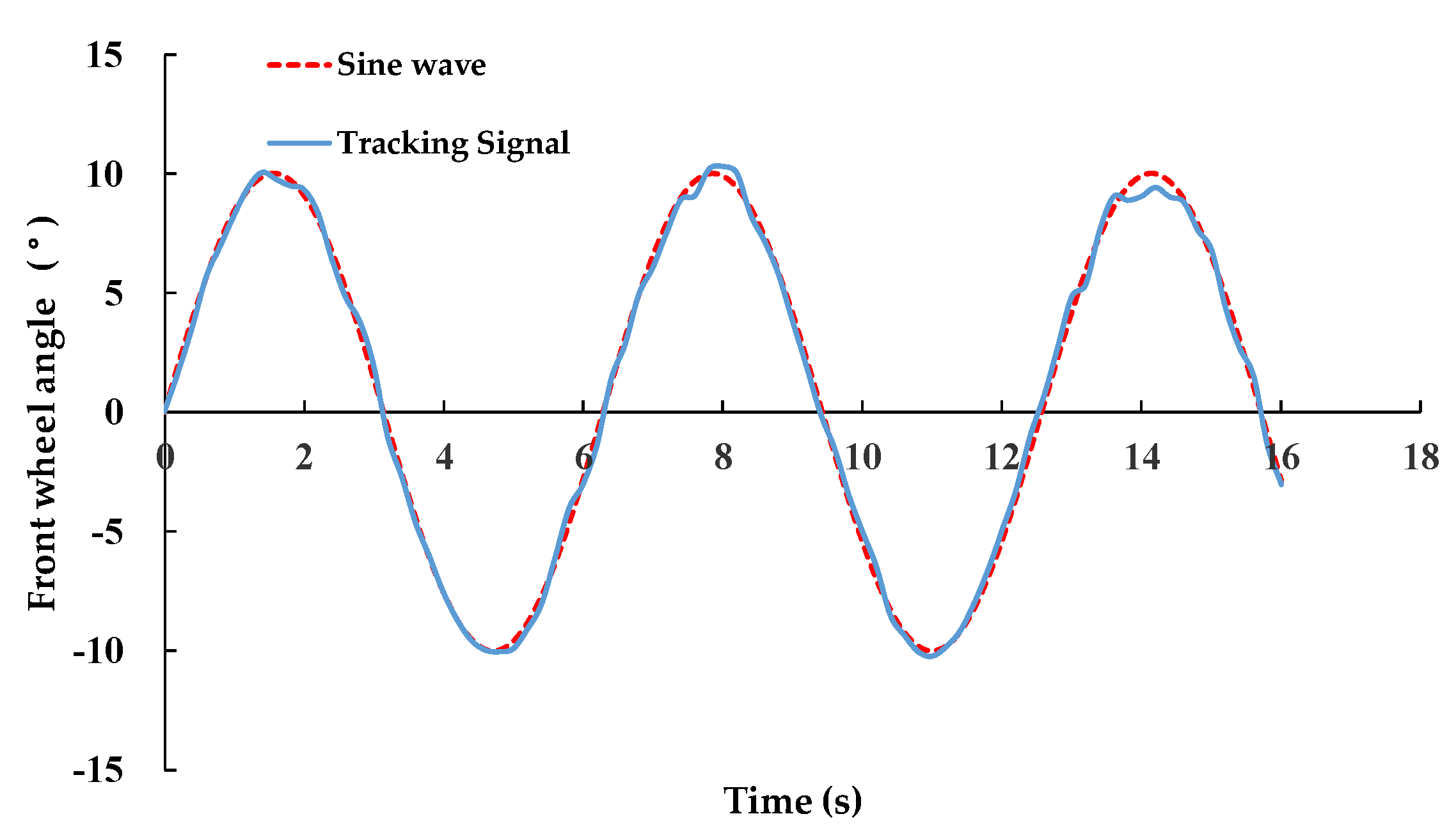
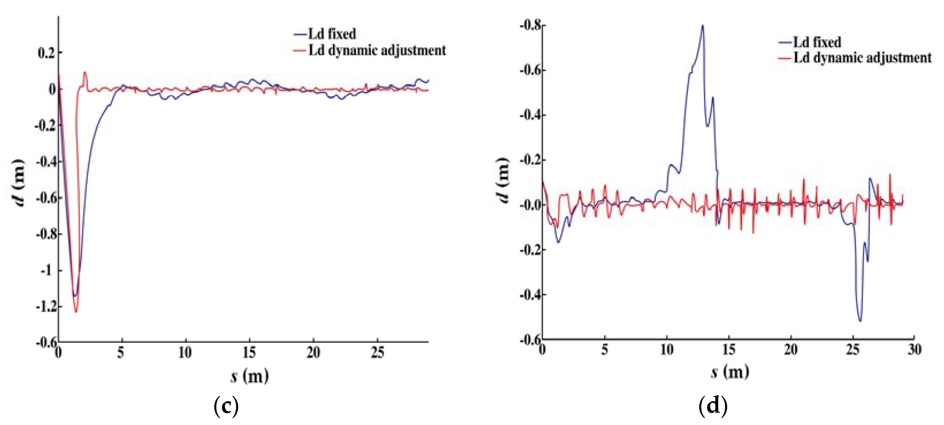
3.1. Path-Tracking Simulation Test

In order to verify the path-tracking control algorithm, the simulation model was established by MATLAB/Simulink, as shown in Figure 14. The model mainly consists of vehicle kinematics model, adaptive pure tracking model, vehicle tracking trajectory generation model and so on.

In the simulation, with set the vehicle speed v₀ = 0.45 m/s and the fixed forward-looking distance 2 m, the initial position of the controlled object is (0 m, 0.1 m), the tracking distance is 30 m. Set two kinds of simulation tracking trajectories. The linear tracking path is shown in Equation (13), and the curve tracking path is shown in Equation (14). The path-tracking simulation results are shown in Figure 15.

$$y_1=0.5x$$

(13)

$$y_2=x\sin 0.2x$$

(14)

It can be seen from Figure 15c that there was a large tracking error in the linear path-tracking in the initial distance. We found that this was because the model sets the initial deviation. After the experiment was adjusted by the controller, when the vehicle was running to about 5.4 m, the pure tracking controller with fixed front view distance reached the basic steady state, and the steady-state average tracking error was 0.089 m. When the vehicle was running to 2.5 m, the adaptive pure tracking controller can achieve steady state, and the steady-state average tracking error was 0.054 m. Therefore, the adaptive pure tracking controller designed in this paper has faster response speed and higher tracking accuracy. It can be seen from Figure 15d that the adaptive pure tracking controller designed in the section with large curvature has better stability than the pure tracking controller with fixed forward-looking distance.

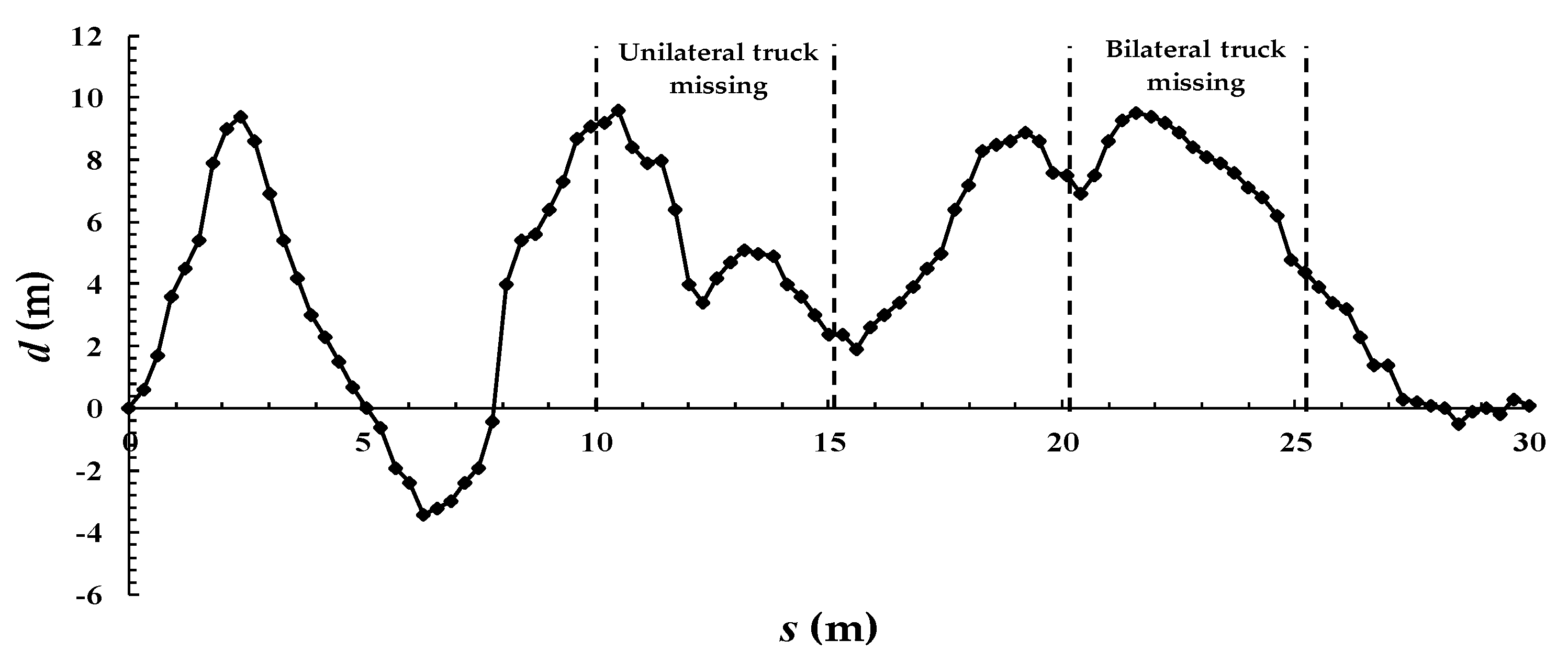
3.2. Feature Map and Navigation Parameter Acquisition Accuracy Test

In order to test the reliability of the system, this paper build a simulation experimental environment in the experimental field of the Northwest A & F University (108°4′30″ E, 34°17′28″ N). And three experiments had been carried out successively which involved navigation path fitting, parameter acquisition accuracy test, vehicle trajectory tracking test. The simulated orchards were arranged in two rows with a spacing of 2.5 m and a row spacing of 4 m, and PVC plastic pipes with a length of 1.2 m were selected to simulate the trunk. The layout of the simulated test scene was similar to the real orchard environment in terms of soil environment, trunk characteristics and trunk arrangement. As shown in Figure 16a, the absolute coordinate system XOY was established with the tree P as a reference, 2 m to the left and 2.5 m to the rear as the origin O. In Figure 16b, the circumference of the simulated fruit tree trunk was measured with a tape measure at the same height as the 2D laser, and the diameter of the tree was obtained to be 0.04 m. The test platform was the hardware system described in Section 2.1.

We placed the test platform statically to capture 2D laser point data at the center of the simulated orchard environment. We placed tree branches as noise disturbance in the driving area of the test platform. The method of fruit tree position information determination in Section 2.2 was used to process the laser point cloud data. According to the actual simulated environmental parameters, take the left and right three fruit trees as the target, set the distance threshold ρ_max = 10 m, x_max = 2.5 m, the number of adjacent points k = 5. The laser point cloud figure after distance threshold processing was shown in Figure 17a; the laser point cloud figure after filter processing was shown in Figure 17b. As shown in Figure 17c, the red points were actual points of trunk, the black points were prediction points of trunk. The method of Section 2.3 was used to fit navigation path and obtain navigation control parameter, as show in Figure 17d.

It can be seen from Figure 17b that the number of laser points on the same fruit tree after European clustering was five or six points. The density of laser points was related to the distance from the trunk to the laser and the diameter of it. In this study, laser data processing was carried out with three singles as one cycle. The distance of the furthest trunk was 7.5 m. It was within the range of laser measurement. Since the laser angle resolution was 0.25°, the problem of missing laser data points was small when locating a simulated trunk with a maximum distance of 7.5 m and a diameter of 4 cm. Therefore, it can provide enough laser points support for the extraction of trunk center feature point.

In Figure 17c, the obtained center point feature map of the trunk has no interference points; the error from the actual position of trunk were 6.79 cm, 2.86 cm, 2.67 cm, 2.33 cm, 2.29 cm and 3.01 cm, from left to right and bottom to top, the average error was 3.325 cm. The results show that the method of obtaining the center point feature map of trunk meets the requirements of positioning accuracy. The linear regression fitting R² of the navigation path was 0.988, which is close to 1. The results show that the method of extracting the navigation path was accurate and reliable.

This experiment puts the test platform in static simulation 2D laser point data at any position in the simulated orchard environment; the heading deviation and lateral deviation obtained by human measurement were taken as the true value. The result is a measured value. The detection range θ is [−30°, 30°], with a sampling interval of 5°. In order to avoid random errors caused by human operation, three tests were performed for each position to obtain an average value as the calculated heading deviation and calculation at that angle. The test results were shown in

Table 4. Positioning accuracy test results.

Serial Number	θ (°)			Δd (cm)
	Actual Value	Measurements	Error
1	−30	−30.13	0.13	2.75
2	−25	−25.40	−0.40	−2.18
3	−20	−19.09	−0.91	1.62
4	−15	−14.34	−0.66	1.04
5	−10	−10.57	0.57	−2.00
6	−5	−5.88	0.88	−2.14
7	0	0.89	0.89	4.66
8	5	4.45	−0.55	−1.06
9	10	10.58	0.58	−1.14
10	15	14.24	−0.76	2.88
11	20	19.05	−0.95	−2.71
12	25	24.17	−0.83	2.20
13	30	30.75	0.75	−1.17
MAD (m)			0.682	2.119
SD (m)			0.237	1.010

. The mean absolute deviation (MAD) and the standard deviation (SD) were used to evaluate and analyze experiment data.

It can be seen from Table 4 that the maximum deviation of the heading angle is 0.95°, the MAD of heading angle θ was 0.682°, the SD of heading angle θ was 0.237°. The lateral deviation d maximum error was 4.66 cm, the MAD was 2.119 cm and the SD was 1.010 cm. The method proposed was used to obtain the navigation path identification and navigation parameter acquisition, which can meet the accuracy requirements of the experimental platform in the orchard autonomous navigation operation.

3.3. Path-Tracking Accuracy Test

The test platform was automatically driven at a speed of 0.45 m/s, the test distance was 30 m and the measurement was carried out at intervals of 30 cm. The test was carried out in 5 groups; the test section of the unilateral fruit tree was missing at a driving distance of 10 m–15 m. At 20 m–25 m, the test section of the bilateral fruit trees was missing. The results after each test were shown in

Table 5. Navigation field test results.

Number	Maximum Deviation (m)	AVG Deviation (m)	SD Deviation (m)
1	0.09	0.05	0.05
2	0.13	0.08	0.04
3	−0.07	−0.04	0.03
4	−0.10	0.04	0.03
5	0.09	−0.03	0.02
MAD (m)	0.096	0.048	0.034

; the average tracking deviation of the test is shown in Figure 18.

As can be seen from Table 4, the maximum lateral deviation after the five tests was 0.13 m, the maximum average deviation was 0.08 m, the MAD of maximum deviation was 0.096 m, the MAD of average deviation was 0.048 m and the SD of average deviation was 0.034 m. It can be seen from Figure 18 that the lateral deviation gradually decreases after the vehicle was 2.5 m. At 5 m, the lateral deviation tends to zero, and then the lateral deviation gradually increases. At 10.6 m, the average maximum lateral deviation was 0.096 m., The deviation fluctuates continuously, and the lateral deviation was basically 0 m at 30 m. At the same time, we can observe that the variation of lateral deviation was not increased due to the loss of fruit trees. Therefore, the effect of missing fruit trees on the accuracy of the navigation control system proposed in this paper was not obvious, indicating that the system has good accuracy and robustness.

4. Conclusions

In order to achieve autonomous driving and path-tracking of vehicles in complex standardized orchards that involve high noise and interference between rows of fruit trees, an automatic vehicle navigation method based on 2D lasers was developed for standardized orchards under complex disturbance environments. This study presents a filtering algorithm based on Euclidean clustering algorithms by analyzing different types of orchard interference points. The algorithm can effectively eliminate noise generated by small disturbances in the orchard by setting different thresholds, thus greatly improving positioning accuracy. Considering prior knowledge of plant spacing, row spacing and trunk diameter, a topographic map of orchard trees’ center was extracted and a target navigation path with higher precision was fit, based on least square methods and geometric linear fitting. It reduces the computation of data processing and complex mathematical models. At the same time, in the pure tracking model, fuzzy control was used to realize the adaptive adjustment of the forward-looking distance. Additionally, the orchard 2D laser automatic navigation system based on agricultural electric vehicle was designed, and its robustness and control accuracy were verified by experiments. This study satisfies the precision requirements of orchard vehicle automatic navigation and provides guidance and suggestions for the industrial application of laser navigation with high precision and low cost in the standardized orchard planting industry.

References

1. Zhao, Y.; Xiao, H.; Mei, S.; Song, Z.; Ding, W.; Jin, Y.; Hang, Y.; Xia, X.; Yang, G. Current status and development strategies of orchard mechanization production in China. J. Chin. Agric. Univ. 2017, 22, 116–127. [Google Scholar]
2. Gao, X.; Li, J.; Fan, L.; Zhou, Q.; Yin, K.; Wang, J.; Song, C.; Huang, L.; Wang, Z. Review of Wheeled Mobile Robots’ Navigation Problems and Application Prospects in Agriculture. IEEE Access 2018, 6, 49248–49268. [Google Scholar] [CrossRef]
3. Shamshiri, R.R.; Weltzien, C.; Hameed, I.A.; Yule, I.J.; Grift, T.E.; Balasundram, S.K.; Pitonakova, L.; Ahmad, D.; Chowdhary, G. Research and development in agricultural robotics: A perspective of digital farming. Int. J. Agric. Biol. Eng. 2018, 11, 1–14. [Google Scholar] [CrossRef]
4. Blok, P.M.; Van Boheemen, K.; Van Evert, F.K.; IJsselmuiden, J.; Kim, G.H. Robot navigation in orchards with localization based on Particle filter and Kalman filter. Comput. Electron. Agric. 2019, 157, 261–269. [Google Scholar] [CrossRef]
5. Radcliffe, J.; Cox, J.; Bulanon, D.M. Machine vision for orchard navigation. Comput. Ind. 2018, 98, 165–171. [Google Scholar] [CrossRef]
6. Ye, Y.; He, L.; Wang, Z.; Jones, D.; Hollinger, G.A.; Taylor, M.E.; Zhang, Q. Orchard manoeuvring strategy for a robotic bin-handling machine. Biosyst. Eng. 2018, 169, 85–103. [Google Scholar] [CrossRef]
7. Keicher, R.; Seufert, H. Automatic guidance for agricultural vehicles in Europe. Comput. Electron. Agric. 2000, 25, 169–194. [Google Scholar] [CrossRef]
8. Yayan, U.; Yucel, H.; Yazici, A. A Low Cost Ultrasonic Based Positioning System for the Indoor Navigation of Mobile Robots. J. Intell. Robot. Syst. 2015, 78, 541–552. [Google Scholar] [CrossRef]
9. Ortiz, B.V.; Balkcom, K.B.; Duzy, L.; Van Santen, E.; Hartzog, D.L. Evaluation of agronomic and economic benefits of using RTK-GPS-based auto-steer guidance systems for peanut digging operations. Precis. Agric. 2013, 14, 357–375. [Google Scholar] [CrossRef]
10. Yin, X.; Du, J.; Noguchi, N.; Yang, T.; Jin, C. Development of autonomous navigation system for rice transplanter. Int. J. Agric. Biol. Eng. 2018, 11, 89–94. [Google Scholar] [CrossRef] [Green Version]
11. Xiong, B.; Zhang, J.; Qu, F.; Fan, Z.; Wang, D.; Li, W. Navigation Control System for Orchard Spraying Machine Based on Beidou Navigation Satellite System. Trans. Chin. Soc. Agric. Mach. 2017, 48, 45–50. [Google Scholar]
12. Liu, L.; Mei, T.; Niu, R.; Wang, J.; Liu, Y.; Chu, S. RBF-Based Monocular Vision Navigation for Small Vehicles in Narrow Space below Maize Canopy. Appl. Sci. 2016, 6, 182. [Google Scholar] [CrossRef] [Green Version]
13. Bengochea-Guevara, J.M.; Conesa-Muñoz, J.; Andújar, D.; Ribeiro, A. Merge Fuzzy Visual serving and GPS-based planning to obtain a proper navigation behavior for a small crop-inspection robot. Sensors 2016, 16, 276. [Google Scholar] [CrossRef]
14. Matthies, L.; Kelly, A.; Litwin, T.; Tharp, G. Obstacle Detection for Unmanned Ground Vehicles: A Progress Report. In Proceedings of the Intelligent Vehicles 95 Symposium, Detroit, MI, USA, 25–26 September 1995; IEEE: Barcelona, Spain, 1995; pp. 66–71. [Google Scholar]
15. Zhai, Z.; Zhu, Z.; Du, Y.; Song, Z.; Mao, E. Multi-crop-row detection algorithm based on binocular vision. Biosyst. Eng. 2016, 150, 89–103. [Google Scholar] [CrossRef]
16. Zhang, S.; Wang, Y.; Zhu, Z.; Li, Z.; Du, Y.; Mao, E. Tractor Path Tracking Control Based on Binocular Vision. Inf. Process. Agric. 2018, 5, 422–432. [Google Scholar] [CrossRef]
17. Milella, A.; Reina, G. 3D reconstruction and classification of natural environments by an autonomous vehicle using multi-baseline stereo. Intell. Serv. Robot. 2014, 7, 79–92. [Google Scholar] [CrossRef]
18. Zhao, H.; Shibasaki, R. Reconstructing a textured CAD model of an urban environment using vehicle-borne laser range scanners and line cameras. Mach. Vis. Appl. 2003, 14, 35–41. [Google Scholar] [CrossRef]
19. Narvaez, F.J.Y.; Del Pedregal, J.S.; Prieto, P.A.; Torres-Torriti, M.; Cheein, F.A.A. LiDAR and thermal images fusion for ground-based 3D characterisation of fruit trees. Biosyst. Eng. 2016, 151, 479–494. [Google Scholar] [CrossRef]
20. Wang, C.; Wang, J.; Li, C.; Ho, D.; Cheng, J.; Yan, T.; Meng, L.; Meng, M.Q.H. Safe and Robust Mobile Robot Navigation in Uneven Indoor Environments. Sensors 2019, 19, 2993. [Google Scholar] [CrossRef] [Green Version]
21. Asvadi, A.; Premebida, C.; Peixoto, P.; Nunes, U. 3D Lidar-based static and moving obstacle detection in driving environments: An approach based on voxels and multi-region ground planes. Robot. Auto Syst. 2016, 83, 299–311. [Google Scholar] [CrossRef]
22. Tuley, J.; Vandapel, N.; Hebert, M. Analysis and removal of artifacts in 3-D LADAR data. In Proceedings of the 2005 IEEE International Conference on Robotics and Automation (ICRA 2005), Barcelona, Spain, 18–22 April 2005; IEEE: Barcelona, Spain, 2005; pp. 2203–2210. [Google Scholar]
23. Hrubos, M.; Nemec, D.; Janota, A.; Pirnik, R.; Bubenikova, E.; Gregor, M.; Juhasova, B.; Juhas, M. Sensor fusion for creating a three-dimensional model for mobile robot navigation. Int. J. Adv. Robot. Syst. 2019, 16, 1–12. [Google Scholar] [CrossRef]
24. Zhao, T.; Noguchi, N.; Yang, L.; Ishii, K.; Chen, J. Development of uncut crop edge detection system based on laser rangefinder for combine harvesters. Int. J. Agric. Biol. Eng. 2016, 9, 21–28. [Google Scholar]
25. Barawid, O.C.; Mizushima, A.; Ishii, K.; Noguchi, N. Development of an Autonomous Navigation System using a Two-dimensional Laser Scanner in an Orchard Application. Biosyst. Eng. 2007, 96, 139–149. [Google Scholar] [CrossRef]
26. Liu, P.; Chen, J.; Zhang, M. Automatic control system of orchard tractor based on laser navigation. Trans. Chin. Soc. Agric. Eng. 2011, 27, 196–199. [Google Scholar]
27. Chen, J.; Jiang, H.; Liu, P.; Zhang, Q. Navigation Control for Orchard Mobile Robot in Curve Path. Trans. Chin. Soc. Agric. Mach. 2012, 43, 179–182+187. [Google Scholar]
28. Thanpattranon, P.; Ahamed, T.; Takigawa, T. Navigation of autonomous tractor for orchards and plantations using a laser range finder: Automatic control of trailer position with tractor. Biosyst. Eng. 2016, 147, 90–103. [Google Scholar] [CrossRef]
29. Bayar, G.; Bergerman, M.; Koku, A.B.; Konukseven, E.I. Localization and control of an autonomous orchard vehicle. Comput. Electron. Agric. 2015, 115, 118–128. [Google Scholar] [CrossRef] [Green Version]
30. Kukko, A.; Kaasalainen, S.; Litkey, P. Effect of incidence angle on laser scanner intensity and surface data. Appl. Optics. 2008, 47, 986–992. [Google Scholar] [CrossRef]
31. Soudarissanane, S.; Lindenbergh, R.; Menenti, M.; Teunissen, P. Scanning geometry: Influencing factor on the quality of terrestrial laser scanning points. ISPRS J. Photogramm. Remote Sens. 2011, 66, 389–399. [Google Scholar] [CrossRef]
32. Lichti, D.D.; Harvey, B.R. The effects of reflecting surface properties on time-off light laser scanner measurements. In Geospatial Theory, Processing and Applications; ISPRS: Ottawa, ON, Canada, 2002; Volume XXXIV, Part 4-IV. [Google Scholar]
33. Voegtle, T.; Schwab, I.; Landes, T. Influences of different materials on the measurements of a terrestrial laser scanner (TLS). In Proceedings of the International Archives of Photogrammetry, Remote Sensing and Spatial Information Sciences, Beijing, China, 3–11 July 2008; Volume XXXVII, Part B5. pp. 1061–1066. [Google Scholar]
34. Urbančič, T.; Koler, B.; Stopar, B.; Kosmatin Fras, M. Quality analysis of the sphere parameters determination in terrestrial laser scanning. Geod. Vestn. 2014, 58, 11–27. [Google Scholar] [CrossRef]
35. Ai, C.; Lin, H.; Wu, D.; Feng, Z. Path planning algorithm for plant protection robots in vineyard. Trans. Chin. Soc. Agric. Eng. 2018, 34, 77–85. [Google Scholar]
36. Xue, J.; Zhang, S. Navigation of an Agricultural Robot Based on Laser Radar. Trans. Chin. Soc. Agric. Mach. 2014, 45, 55–60. [Google Scholar]
37. Zhang, C.; Yong, L.; Chen, Y.; Zhang, S.; Ge, L.; Wang, S.; Li, W. A Rubber-Tapping Robot Forest Navigation and Information Collection System Based on 2D LiDAR and a Gyroscope. Sensors 2019, 19, 2136. [Google Scholar] [CrossRef] [PubMed] [Green Version]
38. Kayacan, E.; Kayacan, E.; Ramon, H.; Saeys, W. Towards agrobots: Identification of the yaw dynamics and trajectory tracking of an autonomous tractor. Comput. Electron. Agric. 2015, 115, 78–87. [Google Scholar] [CrossRef] [Green Version]
39. Xue, J.; Zhang, L.; Grift, T.E. Variable field-of-view machine vision based row guidance of an agricultural robot. Comput. Electron. Agric. 2012, 84, 85–91. [Google Scholar] [CrossRef]
40. Zhang, S.; Liu, J.; Du, Y.; Zhu, Z.; Mao, E.; Song, Z. Method on automatic navigation control of tractor based on speed adaptation. Trans. Chin. Soc. Agric. Eng. 2017, 33, 48–55. [Google Scholar]
41. Conlter, R.C. Implementation of the Pure Pursuit Path Tracking Algorithm: Technical Report; Camegie Mellon University: Pittsburgh, PA, USA, 1992. [Google Scholar]
42. Liu, J.K. Intelligent Control, 4th ed.; Electronic Industry Press: Beijing, China, 2017; pp. 39–41. [Google Scholar]
Figure 1. Test platform composition: (A) 2D laser; (B) Stm32F103; (C): automatic travel switches; (D) main controller PC; (E) tracking device; (F) 121 power supply; (G) steering system; (H) front wheel angle system.
Applsci 10 02763 g001
Figure 2. The principle of system.
Applsci 10 02763 g002
Figure 3. Test platform left and right steering step response curve results.
Applsci 10 02763 g003
Figure 4. Sine wave signal tracking results.
Applsci 10 02763 g004
Figure 5. Laser scanning Cartesian coordinate system.
Applsci 10 02763 g005
Figure 6. Laser data interference point type: (a) laser data cross-line interference point, (b) orbital noise between orchards.
Applsci 10 02763 g006aApplsci 10 02763 g006b
Figure 7. Extraction of the center position of the fruit tree trunk.
Applsci 10 02763 g007
Figure 8. Navigation information parameter extraction schematic.
Applsci 10 02763 g008
Figure 9. Schematic diagram of orchard vehicle path-tracking control system.
Applsci 10 02763 g009
Figure 10. Vehicle kinematics model. Note: M (xr, yr) and N (xf, yf) are the coordinates of the axle of the rear axle and the front axle of the vehicle respectively; P is the instantaneous steering center of the vehicle; Φ is the heading angle of the current position of the vehicle (rad); δ is the front turning angle (rad); vr is the center speed of the rear axle of the vehicle (m·s−1); vf is the center speed of the front axle of the vehicle (m·s−1); l is the wheelbase (m); R is the turning radius of the vehicle (m).
Applsci 10 02763 g010
Figure 11. Pure pursuit model. Note: S is the navigation tracking path; G (xg, yg) is the target point on the path; O is the turning center; γ is the turning rate of the vehicle (m−1); Ld is the forward looking distance (m); R is the instantaneous turning radius (m); d is Lateral deviation (m); θ is the heading deviation (rad); v is the forward speed of the vehicle (m·s−1); l is the vehicle wheelbase (m); δ is the front wheel angle (rad); Ψ is the angle of course change when the vehicle reaches the target point along the steering arc (rad).
Applsci 10 02763 g011
Figure 12. The distribution of the membership function. (a) lateral deviation membership function expression. (b) heading deviation membership function expression. (c) forward-viewing distance membership function expression.
Applsci 10 02763 g012
Figure 13. Fuzzy control surface.
Applsci 10 02763 g013
Figure 14. Path-tracking simulation block diagram.
Applsci 10 02763 g014
Figure 15. Simulation results test charts. (a) Straight path-tracking simulation results. (b) Curved path-tracking simulation results. (c) Linear path-tracking simulation error graph. (d) Curved path-tracking simulation error graph.
Applsci 10 02763 g015aApplsci 10 02763 g015b
Figure 16. Actual test simulation site. (a) position measurement. (b) diameter measurement.
Applsci 10 02763 g016
Figure 17. Navigation path acquisition process. (a) laser point cloud image after distance threshold processing. (b) laser point cloud image after statistical filtering. (c) feature map of center point of fruit tree trunk. (d) navigation path fit results.
Applsci 10 02763 g017
Figure 18. Variation of average deviation of lateral deviation and walking distance.
Applsci 10 02763 g018