Adaptive Robust Force Position Control for Flexible Active Prosthetic Knee Using Gait Trajectory

Featured Application

Active prosthetic knees are integrated functional applications used clinically to empower and assist natural human rehabilitation for the elderly or disabled users. In this paper, an adaptive robust force position control for flexible active prosthetic knee using gait trajectory is proposed to empower and assist natural human motion, providing an optimized approach for further development of prosthetic knee.

Abstract

Active prosthetic knees (APKs) are widely used in the past decades. However, it is still challenging to make them more natural and controllable because: (1) most existing APKs that use rigid actuators have difficulty obtaining more natural walking; and (2) traditional finite-state impedance control has difficulty adjusting parameters for different motions and users. In this paper, a flexible APK with a compact variable stiffness actuator (VSA) is designed for obtaining more flexible bionic characteristics. The VSA joint is implemented by two motors of different sizes, which connect the knee angle and the joint stiffness. Considering the complexity of prothetic lower limb control due to unknown APK dynamics, as well as strong coupling between biological joints and prosthetic joints, an adaptive robust force/position control method is designed for generating a desired gait trajectory of the prosthesis. It can operate without the explicit model of the system dynamics and multiple tuning parameters of different gaits. The proposed model-free scheme utilizes the time-delay estimation technique, sliding mode control, and fuzzy neural network to realize finite-time convergence and gait trajectory tracking. The virtual prototype of APK was established in ADAMS as a testing platform and compared with two traditional time-delay control schemes. Some demonstrations are illustrated, which show that the proposed method has superior tracking characteristics and stronger robustness under uncertain disturbances within the trajectory error in $\pm 0.5$ degrees. The VSA joint can reduce energy consumption by adjusting stiffness appropriately. Furthermore, the feasibility of this method was verified in a human–machine hybrid control model.

1. Introduction

In the past decades, millions of people have had problems with the motion ability of their lower limbs due to wars, diseases, traffic accidents, and natural disasters. In particular, some of them have lost their ability to work and been prevented from engaging in normal social contact [1]. Physical disability significantly reduces their quality of life and puts them under high physical and mental stress. Because the current medical level cannot make the limb regenerate, the prostheses for these amputees have become an essential means to compensate for the loss of limbs. Traditional mechanical knee prostheses cannot bring about a significant change in the lives of amputees because of unnatural walking, great physical exertion, and poor wearing experience of patients. Thanks to advances in actuation, microembedded computing, miniaturized sensing, energy storage, and automatic pattern recognition, many rehabilitative robots have been developed to help and recover human movement [2,3].

To solve these limitations, APK, as a lower limb prosthesis, has drawn increasing research interests to help people deal with walking disabilities in the past years. Compared to a conventional passive prosthesis that has the shortcomings of inability to generate mechanical power and the lack of sensory feedback, APK improves the similarity of able-bodied gait, decreases hip work production, and reduces metabolic expenditure [4]. The active prosthesis is different from the passive prosthesis basically by the use of active components for locomotion assistance. Several research works focused on these prostheses and their control [5,6,7,8,9]. Sup et al. [10] designed a transfemoral prosthesis actuated by a pneumatic cylinder and proposed an impedance-based finite-state controller. Because of the limitations of pneumatic power, an electrically powered robotic prosthesis was developed. In [11], a powered prosthetic knee actuated by brushless dc motor and a hierarchical finite state machine control approach is presented. Ahn et al. [12] discussed the optimization problem for the degree-of-freedom active knee joint actuated by a flat brushless DC electric motor for overcoming complex walking environment. The first commercial active prosthetic knee was the Ossur power knee, which utilized an echo-control strategy to mimic the movements of the subject’s strong side leg. However, these prostheses did not take into account inherent elasticity, and they were affected by the low loads during use. Recent research has been developing an energy-efficient, compliant powered prosthetic knee. Martinez-Villalpando et al. [13] designed dual series-elastic actuators (SEAs) for storing and releasing the energy, where the agonist–antagonist SEAs could lower energy consumption of the active prosthesis. A clutch cable SEA for minimizing electrical energy consumption and satisfying the torque-angle behavior is discussed in [14]. However, the addition of a clutch paralleled with the motor increases the complexity and uncertainty of control. At the same time, a semi-active prosthetic knee for lowering energy consumption by utilizing a lockable parallel spring is proposed in [15]. However, despite promising previous work, there is a need for developing a more flexible bionic, lightweight APK that can be more easily adapted to a variety of activities and different prosthetic users.

In the prostheses mentioned above, the impedance-based finite-state control method is the most popular control scheme. Many teams have successfully implemented it [16,17,18]. For example, when it comes to the variable stiffness mechanisms, a new structure combined with the parallel redundant mechanisms and variable impedance actuator is presented in [19], where a stiffness and position control for two degrees of freedom (DOF) is achieved by three actuators with flexible elements. By utilizing mechanical sensors or biological signals [20,21,22], finite state controllers decompose a gait into several different motion stages and tune a series of corresponding static parameters for each state of every subject. Each motion stage needs at least three parameters: stiffness, damping, and spring balance angle. Thus, the number of tunable parameters dramatically increases with the number of motion states, motion modes, driven joints, and quasi-controlled limbs [23,24]. The tuning process of these parameters is very complicated and time-consuming for the prosthetic user.

More recently, a robust adaptive impedance method based on the nonscalar boundary layer and sliding surface for tracking knee angle is proposed [4], which overcomes the influence of parametric and nonparametric uncertainties. However, to achieve adequate joint trajectory tracking control, a precise robot dynamic model is required. Moreover, the calculation of the APK dynamic model is very complex, and certain model parameters are hard to obtain. The time-delay estimation (TDE) technique presented in [25] is an effective method to reckon nonlinear uncertain systems with time-delayed information. Then, the time-delay control using TDE technique is developed in many robot systems [26,27,28,29,30]. TDC is generally recognized as a simple, efficient, effective, robust model-free scheme. It mainly includes two parts: the TDE part, which is used to reckon the uncertain and nonlinear system dynamics, and the robust control part, which is used to enhance the dynamical performance. Much research has been focused on the latter part of TDC [28,29,31]. Among the many existing robust control methods, sliding mode control has advantages in dealing with uncertain, nonlinear, and bounded external disturbances [32], and has been widely used in TDC. To assure finite-time convergence and avoid the singularity, a model-free nonsingular terminal sliding mode control based on TDE is applied to a robot manipulator in [28]. Recently, an adaptive fractional-order nonsingular terminal sliding mode control with TDE scheme applied in joint tracking of manipulator is discussed [33]. Although the proposed scheme is superior to many other nonsingular terminal sliding mode controls, fractional-order sliding manifold is too complex in the practical applications. The TDC schemes mentioned above make full use of the basic framework of the TDE technique and adopt the improved sliding mode control schemes to ensure the tracking accuracy. However, these schemes mainly focus on a small TDE error. With the external disturbance or parameter variations, the TDE-based controller cannot always guarantee accuracy. Thus, humans encounter many uncertain disturbances in the actual walking.

In this paper, a novel APK with a variable stiffness actuator (VSA) is presented for more flexibility. A new robust TDC scheme for the flexible joint is proposed to achieve improved tracking accuracy based on adaptive nonsingular fast terminal sliding mode control (ANFTSMC) without a sophisticated physical model or multi-tuning parameters. The nonlinear dynamics equation of APK can be effectively eliminated by using TDE. ANFTSMC offers fast adaptation and chattering reduction. To effectively settle the issue of disturbances, an adaptive fuzzy neural network compensator can be added, which can guarantee better robustness in the complex environment.

The primary contributions of this paper are described in the following three points:

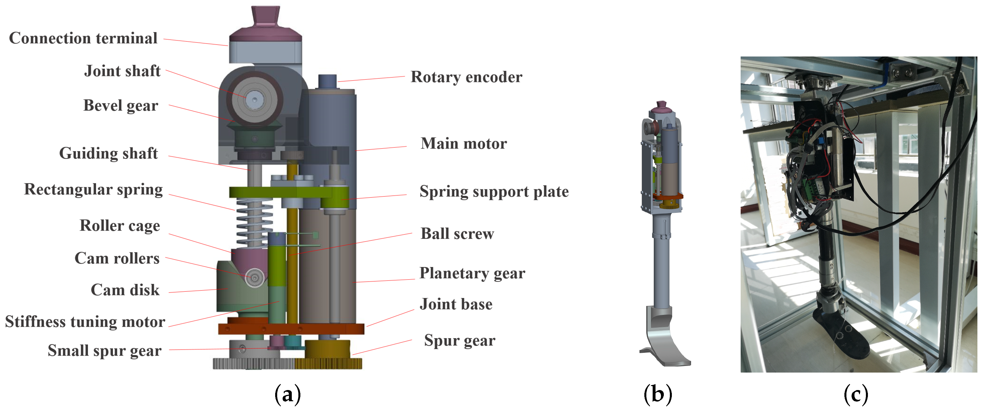
• A novel APK with a variable stiffness actuator (VSA), which can provide the ability to adjust joint stiffness depending on the different gaits, is proposed.
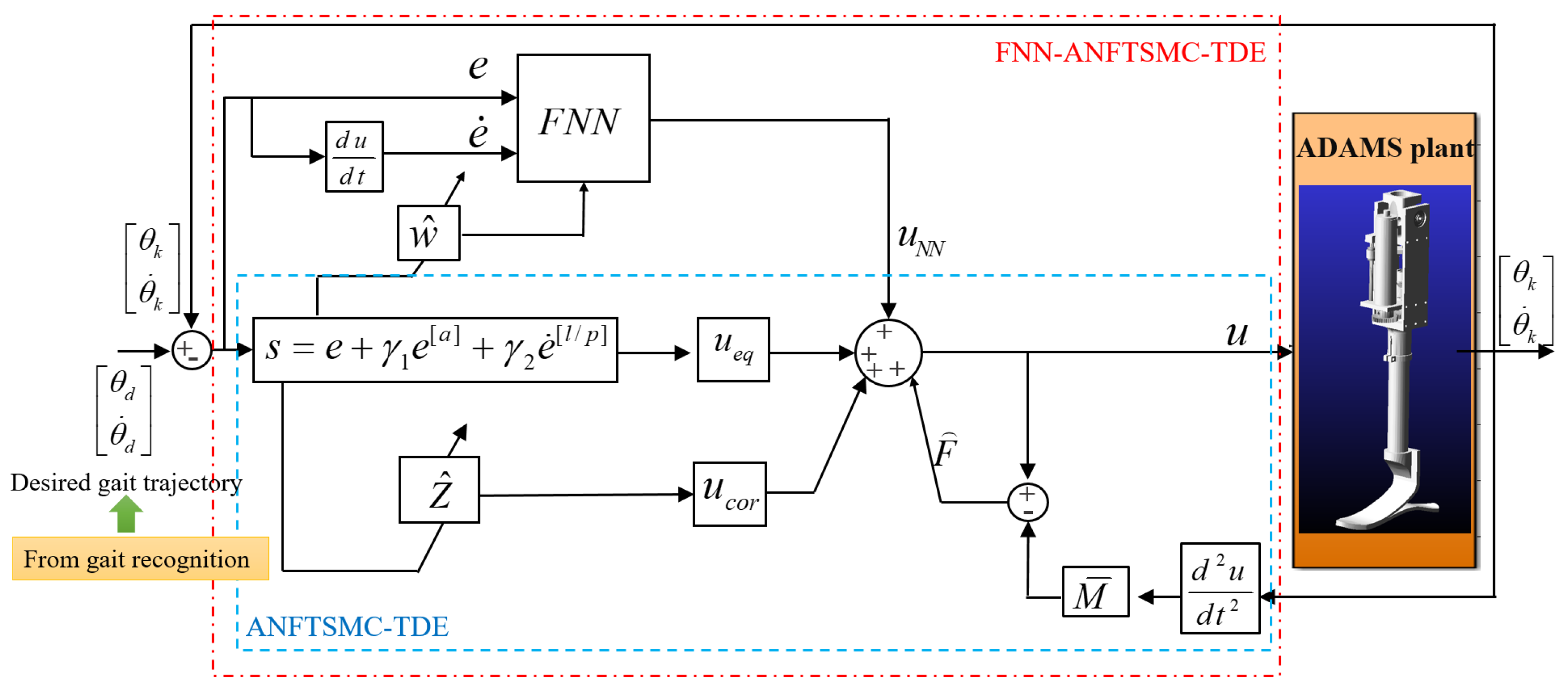
• An adaptive robust force/position controller for flexible APK by using the TDE technique combined with adaptive nonsingular fast terminal sliding mode control and fuzzy neural network is proposed.
• The stability analysis of the control system by Lyapunov stability theory is carried out, and some demonstrations using the virtual prototype illustrate the effectiveness of the proposed algorithm.

The remainder of this paper is structured as follows. Section 2 describes the design of APK with VSA. Section 3 discusses the dynamics model of the APK Joint with VSA. The development of the adaptive robust model-free control is shown in Section 4. Finally, conclusions and discussions are summarized in Section 5.

2. Design of APK with VSA

Compared with rigid actuators, researchers have validated several attractive performances of SEAs, including low mechanical output impedance, impact absorption, and passive mechanical energy storage [34]. The internal elasticity in SEAs makes it possible to convert the force control of the joint into position control [35]. SEAs have been widely utilized in cooperative robots, rehabilitation, and assistive robotics [36,37]. However, a lighter and more flexible bionic knee prosthesis remains a challenge.

Based on the above mentioned, a compact variable stiffness actuator (VSA) is developed for the active prosthetic knee in this paper. Figure 1 illustrates the composition of our VSA active knee joint, and the main parameters of the APK are shown in

Table 1. The main parameters of APK.

Parameter	Value
Maximum knee torque	87 Nm
Range of motion	$-5^{\circ }$∼${115}^{\circ }$
Range of length	48∼52 cm
Total mass	≤2.3 kg

. This structure is improved compared to the previous work [38]. The VSA-Joint utilizes two different size motors to regulate the knee angle and the stiffness of joints, respectively. That is, there are two types of motion in the VSA-Joint: (1) joint rotation provided by the main motor; and (2) stiffness regulating motion provided by stiffness tuning the motor.

For the joint rotation motion, the main motor provides the power for knee joint motion, which firstly is passed on the damping mechanism through a spur gear. The damping mechanism mainly consists of four parts: a cam disk, cam rollers, a roller cage, and a rectangular spring. The cam disk is combined to the joint base and rotates under the drive of the spur gear. Three cam rollers are fixed to the roller cage, and the roller cage is connected to the guiding shaft. There are three curve-surface slots evenly machined on the cam disk along the axial direction. Then, the cam rollers can roll on the slots, and the torque from the cam disk is indirectly transmitted to the guiding shaft; at the same time, the rectangular spring is compressed by the upward motion of the rollers. This mechanism supplies cushion corresponding to the deflection of the flexible joint. The main motion generated by the main motor is implemented to a bevel gear whose driving gear is fixed to the guiding shaft, and the follower gear is connected with the joint shaft. The thigh connection terminal is fixed to the joint shaft. Finally, the main motor drives the knee joint to rotate.

For the stiffness motion, the joint stiffness can be controlled by the stiffness regulator, which involves a stiffness tuning motor, a spring support plate, a ball screw, and a small spur gear. The stiffness tuning motor is utilized to adjust the rectangular spring precompression, which can be decreased or increased by actuating the spring support plate up and down through the ball screw.

3. Dynamics Model of the APK Joint with VSA

In this section, a unilateral above-knee amputee wearing APK is modeled in the sagittal plane. This includes the amputee’s biological hip joint and the proposed APK joint. The dynamics representation is derived from the Euler–Lagrange method [39]. Since biological joints are completely controlled by a human, this section focuses on the dynamics of the prosthetic knee joint.

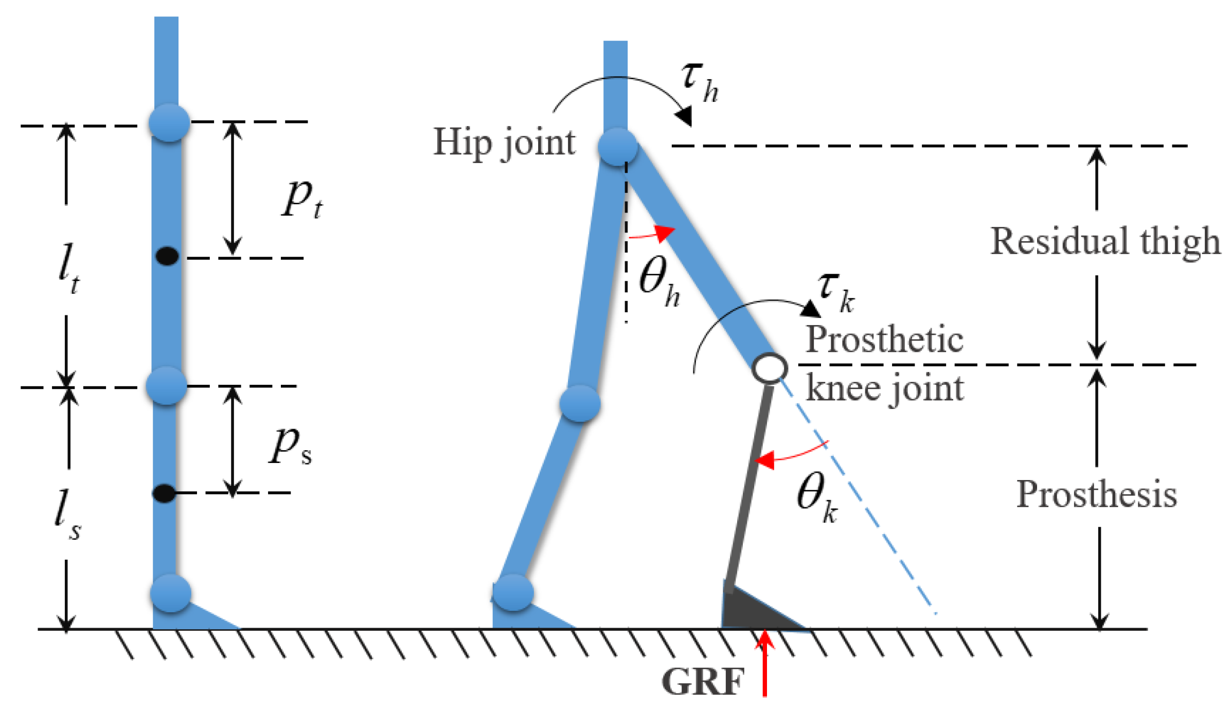
3.1. Dynamic Model of Human–Machine Hybrid System

The APK is installed below the residual thigh of the transfemoral amputees and is connected with the thigh receiving cavity of the patient. Then, a strongly coupled human–machine hybrid system is formed between the human body and the APK during walking. The diagram of a human–machine hybrid system in the sagittal plane is exhibited in Figure 2.

By using Euler–Lagrange method, the dynamic equation of unilateral human–machine hybrid model can be obtained as follows:

$$\mathrm{M}\left(\theta \right)\ddot{\theta }+\mathrm{C}(\theta ,\dot{\theta })\dot{\theta }+\mathrm{G}\left(\theta \right)+{Ø}_e=\tau +{Ø}_G$$

(1)

where $\theta ={\left[{\theta }_h{\theta }_k\right]}^T\in {\mathbb{R}}^2$ denotes joint angle, input torque is represented by $\tau ={\left[{\tau }_h{\tau }_k\right]}^T$ with ${\tau }_h$ the torque of biological hip joint, and ${\tau }_k$ denotes the torque of prosthetic knee. ${\tau }_e={\left[{\tau }_{eh}{\tau }_{ek}\right]}^T$ represent the interactive torque and unknown disturbance caused by movement of other parts of the upper body to lower limb. ${\tau }_G={\left[{\tau }_{Gh}{\tau }_{Gk}\right]}^T$ denotes the torque generated by ground reaction force (GRF) on each joint during support phase. $\mathrm{M}\left(\theta \right)=[M_{hh}{M}_{hk};M_{kh}{M}_{kk}]$ denotes the inertia matrix. $\mathrm{C}(\theta ,\dot{\theta })=[C_{hh}{C}_{hk};C_{kh}{C}_{kk}]$ denote the Coriolis and Centripetal forces matrix. $\mathrm{G}\left(\theta \right)=\left[G_h{G}_k\right]$ represents the gravitational force vector. The dynamic equations and model parameters are detailed as follows:

$$\begin{array}{cc}\hfill \mathrm{M}\left(\theta \right)& =\left[\begin{array}{cc}{M}_{hh}& M_{hk}\\ M_{kh}& M_{kk}\end{array}\right]\hfill \\ \hfill M_{hh}& =m_t{p}_t^2+m_s{l}_s^2+m_s{p}_s^2+2m_s{l}_t{p}_{s}cos\left(2{\theta }_h\right)cos{\theta }_k\hfill \\ \hfill M_{hk}& =-m_s{p}_s^2-m_s{l}_t{p}_{s}cos\left(2{\theta }_h\right)cos{\theta }_s\hfill \\ \hfill M_{kh}& =-m_s{p}_s^2-m_s{l}_t{p}_{s}cos\left(2{\theta }_h\right)cos{\theta }_k\hfill \\ \hfill M_{kk}& =m_s{p}_s^2\hfill \\ \hfill \mathrm{C}(\theta ,\dot{\theta })& =\left[\begin{array}{cc}{C}_{hh}& C_{hk}\\ C_{kh}& C_{kk}\end{array}\right]\hfill \\ \hfill C_{hh}& =-2m_s{l}_t{p}_{s}sin\left(2{\theta }_h\right)cos{\theta }_k{\dot{\theta }}_h-m_s{l}_t{p}_{s}cos\left(2{\theta }_h\right)sin{\theta }_k{\dot{\theta }}_k\hfill \\ \hfill C_{hk}& =m_s{l}_t{p}_{s}cos\left(2{\theta }_h\right)({\dot{\theta }}_k-{\dot{\theta }}_h)\hfill \\ \hfill C_{kh}& =m_s{l}_t{p}_s(2sin\left(2{\theta }_h\right)cos{\theta }_k+cos\left(2{\theta }_h\right)sin{\theta }_k){\dot{\theta }}_h\hfill \\ \hfill C_{kk}& =0\hfill \\ \hfill \mathrm{G}\left(\theta \right)& =\left[\begin{array}{c}{G}_h\\ G_k\end{array}\right]\hfill \\ \hfill G_h& =(m_{t}g{p}_t+m_{s}g{l}_t)sin{\theta }_h-m_{s}g{p}_{s}sin({\theta }_k-{\theta }_h)\hfill \\ \hfill G_k& =m_{s}g{p}_{s}sin({\theta }_k-{\theta }_h)\hfill \end{array}$$

(2)

where $m_s,l_s,p_s$ are the mass of shank, length of shank, and distance between the knee and the centroid of the shank, respectively, and $m_t,l_t,p_t$ are the mass of thigh, length of thigh, and distance between the hip and the centroid of the thigh, respectively.

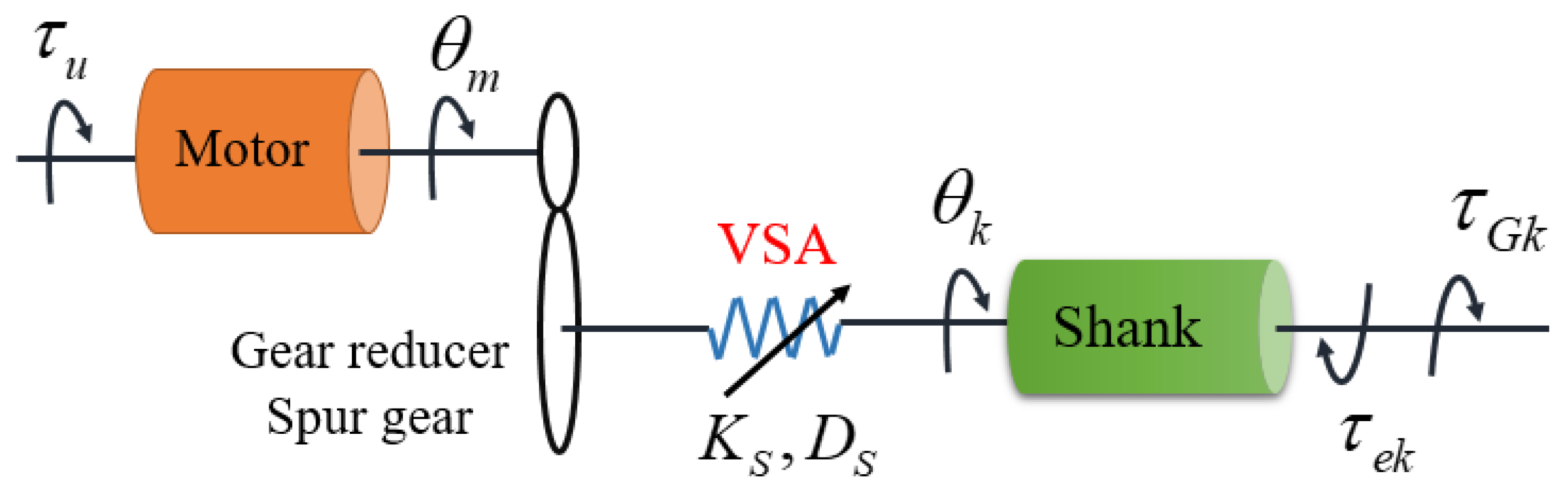
3.2. Dynamic Model of the APK Joint

The hip joint and residual thigh are controlled by human in Figure 2, and the knee joint dynamic model can be extracted from Equation (1):

$$M_{kk}{\ddot{\theta }}_k+C_{kk}{\dot{\theta }}_k+G_k+M_{kh}{\ddot{\theta }}_h+C_{kh}{\dot{\theta }}_h+{Ø}_{ek}={\tau }_k+{Ø}_{Gk}$$

(3)

As can be seen from the above equation, the knee joint dynamic model includes the independent term of the knee joint and the coupled term between the knee joint and the hip joint. Furthermore, the knee joint is driven by VSA, and the dynamic model of the APK joint is also related to the VSA driver. The schematic diagram of the VSA knee joint model is shown in Figure 3.

The dynamic model of the APK with VSA, which is shown in Figure 3, can be described as follows:

$${\mathrm{I}}_{\mathrm{m}}{\ddot{\theta }}_m+{\mathrm{D}}_{\mathrm{m}}{\dot{\theta }}_m={Ø}_u-{Ø}_k$$

(4)

$${Ø}_k={\mathrm{K}}_s({\theta }_k-{\theta }_m)+{\mathrm{D}}_s({\dot{\theta }}_k-{\dot{\theta }}_m)$$

(5)

where ${\theta }_m$ denotes position of the main motor (hereinafter, called ‘motor’), and ${\theta }_k$ denotes position of the prosthetic knee. ${\mathrm{I}}_{\mathrm{m}}$ represents the motor inertia, ${\mathrm{D}}_{\mathrm{m}}$ denotes the motor damping, ${Ø}_u$ denotes the input torque to the motor, and ${Ø}_k$ denotes joint compliance torque defined in Equation (5). ${\mathrm{K}}_s$ is the joint stiffness and ${\mathrm{D}}_s$ is the joint damping.

From Equations (3)–(5), the dynamic model of VSA-driven APK can be summarized as:

$$\begin{array}{c}\hfill \underset{fromkneejointdynamics}{\underbrace{M_{kk}{\ddot{\theta }}_k+C_{kk}{\dot{\theta }}_k+G_k}}+\underset{frommotordynamics}{\underbrace{{\mathrm{I}}_{\mathrm{m}}{\ddot{\theta }}_m+{\mathrm{D}}_{\mathrm{m}}{\dot{\theta }}_m}}+\underset{fromhipjointcoupleddynamics}{\underbrace{M_{kh}{\ddot{\theta }}_h+C_{kh}{\dot{\theta }}_h}}+{Ø}_{ek}={Ø}_u+{Ø}_{Gk}\end{array}$$

(6)

4. Adaptive Robust Model Free Control

From Equation (6), it is clear that the dynamic model of APK is highly complex and it is impossible to obtain exact parameters. In this section, a robust adaptive model-free control method is presented to realize the force/position control of the APK joint using gait trajectory without an explicit model of the system dynamics.

4.1. System Problem Description

Introducing a gain constant $\overline{\mathrm{M}}$ is into Equation (6), the following dynamics can be obtained:

$${Ø}_u=\overline{\mathrm{M}}{\ddot{\theta }}_k+\mathrm{F}\left(t\right)-{Ø}_{Gk}$$

(7)

where $\mathrm{F}\left(t\right)$ stands for a lumped item containing all nonlinearities and unknown dynamics, and is characterized as

$$\begin{array}{c}\hfill \mathrm{F}\left(t\right)\triangleq (M_{kk}-\overline{\mathrm{M}}){\ddot{\theta }}_k+C_{kk}{\dot{\theta }}_k+G_k+{\mathrm{I}}_{\mathrm{m}}{\ddot{\theta }}_m+{\mathrm{D}}_{\mathrm{m}}{\dot{\theta }}_m+M_{kh}{\ddot{\theta }}_h+C_{kh}{\dot{\theta }}_h+{Ø}_{ek}\end{array}$$

(8)

It is easy to conclude from Equation (8) that $\mathrm{F}\left(t\right)$ is very complicated, and consists of three parts: the power knee joint dynamics including the nonlinear terms and unknown disturbance, the motor dynamics, and the hip joint coupled dynamics. Obviously, it can acquire $\mathrm{F}\left(t\right)$ with the calculation method. $\mathrm{F}\left(t\right)$ can be given by the TDE technique:

$$\mathrm{F}\left(t\right)\cong \widehat{\mathrm{F}}\left(t\right)\triangleq \mathrm{F}(t-T)={Ø}_u(t-T)-\overline{\mathrm{M}}\ddot{\theta }(t-T)+{Ø}_{Gk}(t-T)$$

(9)

where T denotes the sampling period. This method assumes that unknown nonlinear functions do not change significantly if T is sufficiently small [26,28,29,33].

4.2. Design of Control Based on ANFTSMC

Let $x_1={\theta }_k$ and $x_2={\dot{\theta }}_k$. Equation (7) is rearranged into a state space form:

$$\begin{array}{c}{\dot{x}}_1=x_2;\hfill \\ {\dot{x}}_2={\overline{\mathrm{M}}}^{-1}(u-\mathrm{F}\left(t\right)+{Ø}_{Gk});\hfill \\ y=x_1;\hfill \end{array}$$

(10)

where $u={Ø}_u$. To realize the desired gait trajectory ${\theta }_d$, we define $x_d={\theta }_d$; then, the tracking error is obtained as

$$e=x_1-x_d$$

(11)

The NFTSMC design process contains two steps. Firstly, a suitable non-singular fast terminal sliding surface is designed [29]:

$$s=e+{\gamma }_1{e}^{\left[a\right]}+{\gamma }_2{\dot{e}}^{\left[\frac{m}{n}\right]}$$

(12)

where ${\gamma }_1$ and ${\gamma }_2$ are positive constants, m and n must satisfy the condition $1<m/n<2$ and are generally positive odd numbers, and the value of a satisfies $a>m/n$. $e^{\left[c\right]}={\left|e\right|}^{c}sign\left(e\right)(c>0)$, where $sign(·)$ means symbolic function.

Secondly, to propel the system state toward the sliding surface within limited time, it is necessary to preserve the ideal sliding motion, which means $\dot{s}=0$ [29], and thus

$$\dot{s}=\dot{e}+{\gamma }_1{a\left|e\right|}^{a-1}\dot{e}+{\gamma }_2\frac{m}{n}{\left|\dot{e}\right|}^{\frac{m}{n}-1}({\ddot{x}}_1-{\ddot{x}}_d)$$

(13)

Substituting Equation (7) into Equation (13), we can have

$$\begin{array}{c}\hfill \dot{s}=\dot{e}+{\gamma }_1{a\left|e\right|}^{a-1}\dot{e}+{\gamma }_2\frac{m}{n}{\left|\dot{e}\right|}^{\frac{m}{n}-1}({\overline{\mathrm{M}}}^{-1}u-{\overline{\mathrm{M}}}^{-1}\mathrm{F}\left(t\right)+{\overline{\mathrm{M}}}^{-1}{Ø}_{Gk}-{\ddot{x}}_d)\end{array}$$

(14)

where u can be designed as [40]:

$$u=u_{eq}+u_{cor}$$

(15)

where $u_{eq}$ denotes equivalent control law and $u_{cor}$ represents correction control law. $u_{eq}$ is applied to control object component and can be obtained from the ideal sliding motion $\dot{s}=0$.

Substitute Equation ( 15 ) into Equation (14), where $u=u_{eq}$, and solve for $u_{eq}$ as follows:

$$\begin{array}{c}\hfill u_{eq}=-\overline{\mathrm{M}}\frac{1}{{\gamma }_2}\frac{n}{m}(\left({\dot{e}}^{[2-\frac{m}{n}]}\right)+{\gamma }_1{a\left|e\right|}^{a-1}{\dot{e}}^{[2-\frac{m}{n}]})+\widehat{\mathrm{F}}\left(t\right)-{Ø}_{Gk}+\overline{\mathrm{M}}{\ddot{x}}_d\end{array}$$

(16)

To guarantee reaching the sliding surface, conventional $u_{cor}$ is designed [29] as

$$u_{cor}=-\overline{\mathrm{M}}(\eta +Z)sign\left(s\right)$$

(17)

where $\eta >0$ denotes the converging factor and $Z>0$ is the upper bound of disturbances and uncertainties. To ensure the convergence of the system, the sliding gain $\eta +Z$ in Equation (17) must be greater than the superior limit of the perturbation, which is impossible to be acquired in advance in practical applications. However, too large control gain will lead to significant chattering on the switching manifold. To relieve the fundamental chattering, we design an adaptive reaching law to approximate the upper limit $\widehat{Z}$:

$$\dot{\widehat{Z}}=s{\gamma }_2\frac{m}{n}{\left|\dot{e}\right|}^{\frac{m}{n}-1}sign\left(s\right)$$

(18)

Theorem 1.

A nonlinear system Equation (10) with disturbances and uncertainties is considered. If the defined ANFTSMC-TDE control law in Equations (15)–(18) is employed, the convergence and stability of the system are ensured during the whole process.

Proof: Define the Lyapunov function as

$$V_2=V_1+\frac{1}{2\kappa }{\tilde{w}}^2$$

(19)

where $\tilde{w}=w^{*}-\widehat{w}$. Differentiate the Lyapunov function $V_2$, which leads to:

$$\begin{array}{cc}\hfill {\dot{V}}_2& ={\dot{V}}_1+\frac{1}{\kappa }\tilde{w}\dot{\widehat{w}}\hfill \\ \hfill & =s(\dot{e}+{\gamma }_1{a\left|e\right|}^{a-1}\dot{e}+{\gamma }_2\frac{m}{n}|\dot{e}{|}^{\frac{m}{n}-1}({\overline{\mathrm{M}}}^{-1}u-{\overline{\mathrm{M}}}^{-1}\mathrm{F}\left(t\right)\hfill \\ & +{\overline{\mathrm{M}}}^{-1}{Ø}_{Gk}-{\ddot{x}}_d\left)\right)+(\widehat{Z}-Z)\dot{\widehat{Z}}+\frac{1}{\kappa }\tilde{w}\dot{\widehat{w}}\hfill \end{array}$$

(20)

where

$$\begin{array}{cc}\hfill u& =u_{eq}+u_{cor}+u_{NN}\hfill \\ \hfill & =-\overline{\mathrm{M}}\frac{1}{{\gamma }_2}\frac{n}{m}(\left({\dot{e}}^{[2-m/n]}\right)+{\gamma }_1{a\left|e\right|}^{a-1}{\dot{e}}^{[2-m/n]})+\widehat{\mathrm{F}}\left(t\right)\hfill \\ \hfill & -{Ø}_{Gk}+\overline{\mathrm{M}}{\ddot{x}}_d-\overline{\mathrm{M}}(\eta +\widehat{Z})sign\left(s\right)-{\widehat{w}}^T\xi \left(x\right)\hfill \end{array}$$

(21)

Then,

$$\begin{array}{cc}\hfill {\dot{V}}_2& =s(-{\gamma }_2\frac{m}{n}|\dot{e}{|}^{\frac{m}{n}-1}\overline{\mathrm{M}}\tilde{w}\xi \left(x\right)-{\gamma }_2\frac{m}{n}\left|\dot{e}{|}^{\frac{m}{n}-1}(\eta +Z)sign\left(s\right)\right)\hfill \\ & +\overline{\mathrm{M}}s{\gamma }_2\frac{m}{n}{\left|\dot{e}\right|}^{\frac{m}{n}-1}\tilde{w}\xi \left(x\right)\hfill \\ \hfill & =-s\left({\gamma }_2\frac{m}{n}\right|\dot{e}{|}^{\frac{m}{n}-1}(\eta +Z)sign\left(s\right))\hfill \\ \hfill & =-{\gamma }_2\frac{m}{n}|\dot{e}{|}^{\frac{m}{n}-1}(\eta +Z)\left|s\right|\hfill \end{array}$$

(22)

It can be seen that ${\dot{V}}_2\le 0$; therefore, the convergence and stability of the system is confirmed through the Lyapunov criterion. This completes the proof.

Remark 1.

For the nonlinear system in Equation (10), when the sliding variable in Equation (12) is convergent to zero, the system tracking error rapidly approaches zero within limited time. The finite time $t_p$, which is defined as the time from $e\left(t_0\right)\ne 0$ to $e(t_0+t_p)=0$, is determined by [41]:

$$\begin{array}{c}\hfill t_p=\frac{\frac{m}{n}{\left|e\left(t_0\right)\right|}^{1-\frac{n}{m}}}{{\gamma }_1(\frac{m}{n}-1)}·H\left(\frac{n}{m},\frac{\frac{m}{n}-1}{(a-1)\frac{m}{n}};1+\frac{\frac{m}{n}-1}{(a-1)\frac{m}{n}};-{\gamma }_1{\left|e\left(t_0\right)\right|}^{a-1}\right)\end{array}$$

(23)

where $H(·)$ represents a Gauss hypergeometric function.

Remark 2.

The TDE error is bounded by a constant Z that is defined as $\parallel \widehat{F}{\left(t\right)-F\left(t\right)\parallel }_{\infty }\le Z$ when $\overline{\mathrm{M}}$ satisfies the following equation:

$$\parallel I-M_k^{-1}\left(q\right)\overline{M}\parallel <1$$

(24)

The proof details are described in [42]. In practical applications, the value of the gain $\overline{M}$ can be adjusted from a smaller positive one to a larger one until the system starts oscillating. Therefore, it is not difficult to tune $\overline{M}$ to meet the criteria in Equation (24).

To further reduce the chattering effects, the symbolic function sign(s) is changed to the saturation function sat(s) [40]. The correction signal $u_{cor}$ of Equation (17) becomes

$$\begin{array}{cc}\hfill u_{cor}& =-\overline{\mathrm{M}}(\eta +\widehat{Z})sat(s,\sigma )\hfill \\ \hfill & =-\overline{\mathrm{M}}(\eta +\widehat{Z})\left\{\begin{array}{cc}-1\hfill & \mathrm{if}\mathrm{s}<-\sigma \hfill \\ \frac{s}{\sigma }\hfill & \mathrm{if}\mid \mathrm{s}\mid \le \sigma \hfill \\ 1\hfill & \mathrm{if}\mathrm{s}>\sigma \hfill \end{array}\right.\hfill \end{array}$$

(25)

where $\sigma >0$ is the boundary layer thickness.

4.3. Adaptive Fuzzy Neural Network Compensator

If disturbances, uncertainties, and abrupt external forces are too large, TDE estimation error will also change greatly. TDE error is obtained as follow:

$$\xi \left(t\right)=\widehat{F}\left(t\right)-F\left(t\right)$$

(26)

where $\left|\xi \right(t\left)\right|\le Z$. To take advantages of the artificial neural network and fuzzy inference system, a fuzzy neural network is proposed for compensating the TDE error. It has been proved that the fuzzy neural network has a nonlinear function approachability with arbitrary precision [43].

Then, we obtain the new control law:

$$u=u_{eq}+u_{cor}+u_{NN}$$

(27)

where $u_{eq}$ denotes the same designed as in Equation (16), and $u_{NN}$ denotes compensation term. Define $\widehat{\xi }(x,w)$ as the fuzzy approximation function of $\xi \left(t\right)$, and $\widehat{\xi }(x,w)$ can be described as

$$\widehat{\xi }(x,w)=\frac{{\sum }_{i=1}^h{w}_i\left({\prod }_{j=1}^n{\mu }_{A_j^i}\left(x_j\right)\right)}{{\sum }_{i=1}^h\left({\prod }_{j=1}^n{\mu }_{A_j^i}\left(x_j\right)\right)}=w^T\Phi \left(x\right)$$

(28)

where h denotes the total number of fuzzy rules, n is the number of states, and $w={[w_1,w_2,..,w_h]}^T$ is a vector of design parameters. ${\mu }_{A_j^i}\left(x_j\right)=exp(-\frac{\parallel x_j-c_{ji}\parallel }{b_i})$ is the Gaussian function as the membership function of the input variable $x_j$. $c_{ji}$ and $b_i$ are the mean value and standard deviation of the Gaussian function, respectively. $\Phi \left(x\right)={[{\Phi }_1\left(x\right),{\Phi }_2\left(x\right),...,{\Phi }_h\left(x\right)]}^T$ is the fuzzy basis function vector, and defined as

$${\Phi }_i\left(x\right)=\frac{{\prod }_{j=1}^n{\mu }_{A_j^i}\left(x_j\right)}{{\sum }_{i=1}^h\left({\prod }_{j=1}^n{\mu }_{A_j^i}\left(x_j\right)\right)}$$

(29)

Define $w^{*}$ as the optimal weight and the approximation error is described as:

$$\delta =\widehat{\xi }(x,w^{*})-\xi (x,\widehat{w})$$

(30)

and $w^{*}$ should be satisfied with

$$w^{*}=argmi{n}_{\begin{array}{c}w\in \mathsf{\Omega }\end{array}}\left\{sup\right|\widehat{\xi }(x,w)-\xi (x,\widehat{w})\left|\right\}$$

(31)

where $\mathsf{\Omega }$ is the set of w. Combining Equations (27), (16), (25), and (10), the system error function can be attained:

$$\begin{array}{cc}\hfill & \ddot{e}+\frac{1}{{\gamma }_2}\frac{n}{m}({\dot{e}}^{[2-m/n]}+{\gamma }_{1}a{e}^{a-1}{\dot{e}}^{[2-m/n]})+(\eta +\widehat{Z})\hfill \\ \hfill & sat(s\left(t\right),\sigma )={\overline{\mathrm{M}}}^{-1}(\widehat{\Phi }(x,w^{*})-\delta +u_{FNN})\hfill \end{array}$$

(32)

To eliminate the TDE error, i.e., to let $li{m}_{t\to \infty }e\left(t\right)=0$, the following equation should be satisfied:

$$u_{FNN}=-\xi (x,\widehat{w})=-{\widehat{w}}^T\Phi \left(x\right)$$

(33)

The adaptive rate of weight can be designed as follows:

$$\dot{\widehat{w}}=\kappa \overline{\mathrm{M}}s{\gamma }_2\frac{m}{n}{\left|\dot{e}\right|}^{\frac{m}{n}-1}\Phi \left(x\right)$$

(34)

where $\kappa >0$.

Theorem 2.

Considering the nonlinear and unknown system in Equation (10), when the proposed control laws in Equations (27) and (33) with adaptive law in Equation (34) are employed in the whole process, the convergence and stability of the system are guaranteed.

Proof. 

Define the Lyapunov function as follows:

$$V_2=V_1+\frac{1}{2\kappa }{\tilde{w}}^2$$

(35)

where $\tilde{w}=w^{*}-\widehat{w}$. Differentiate the Lyapunov function $V_2$, which leads to:

$$\begin{array}{cc}\hfill {\dot{V}}_2& ={\dot{V}}_1+\frac{1}{\kappa }\tilde{w}\dot{\widehat{w}}\hfill \\ \hfill & =s(\dot{e}+{\gamma }_1{a\left|e\right|}^{a-1}\dot{e}+{\gamma }_2\frac{m}{n}|\dot{e}{|}^{\frac{m}{n}-1}({\overline{\mathrm{M}}}^{-1}u-{\overline{\mathrm{M}}}^{-1}\mathrm{F}\left(t\right)\hfill \\ & +{\overline{\mathrm{M}}}^{-1}{Ø}_{Gk}-{\ddot{x}}_d\left)\right)+(\widehat{Z}-Z)\dot{\widehat{Z}}+\frac{1}{\kappa }\tilde{w}\dot{\widehat{w}}\hfill \end{array}$$

(36)

where

$$\begin{array}{cc}\hfill u& =u_{eq}+u_{cor}+u_{NN}\hfill \\ \hfill & =-\overline{\mathrm{M}}\frac{1}{{\gamma }_2}\frac{n}{m}(\left({\dot{e}}^{[2-m/n]}\right)+{\gamma }_1{a\left|e\right|}^{a-1}{\dot{e}}^{[2-m/n]})+\widehat{\mathrm{F}}\left(t\right)\hfill \\ \hfill & -{Ø}_{Gk}+\overline{\mathrm{M}}{\ddot{x}}_d-\overline{\mathrm{M}}(\eta +\widehat{Z})sign\left(s\right)-{\widehat{w}}^T\xi \left(x\right)\hfill \end{array}$$

(37)

Then,

$$\begin{array}{cc}\hfill {\dot{V}}_2& =s(-{\gamma }_2\frac{m}{n}|\dot{e}{|}^{\frac{m}{n}-1}\overline{\mathrm{M}}\tilde{w}\xi \left(x\right)-{\gamma }_2\frac{m}{n}\left|\dot{e}{|}^{\frac{m}{n}-1}(\eta +Z)sign\left(s\right)\right)\hfill \\ & +\overline{\mathrm{M}}s{\gamma }_2\frac{m}{n}{\left|\dot{e}\right|}^{\frac{m}{n}-1}\tilde{w}\xi \left(x\right)\hfill \\ \hfill & =-s\left({\gamma }_2\frac{m}{n}\right|\dot{e}{|}^{\frac{m}{n}-1}(\eta +Z)sign\left(s\right))\hfill \\ \hfill & =-{\gamma }_2\frac{m}{n}|\dot{e}{|}^{\frac{m}{n}-1}(\eta +Z)\left|s\right|\hfill \end{array}$$

(38)

It can be seen that ${\dot{V}}_2\le 0$; therefore, the convergence and stability of the system is confirmed through the Lyapunov criterion. This completes the proof.  □

We constructed a virtual prototype with ADAMS to testify to the significance of the proposed method. The architecture of the controller is shown in Figure 4. In the ANFTSMC-TDE sub-controller, the nonlinearity and uncertainty of APK dynamics are estimated by TDE technique. A fuzzy neural network is thus designed to compensate for TDE error. First, we verified the effectiveness and robustness of the proposed method in the swing phase comparing with the other two traditional TDE methods. Then, we validated the performance of VSA under different stiffnesses. Finally, we constructed a human–machine hybrid model to confirm the proposed method.

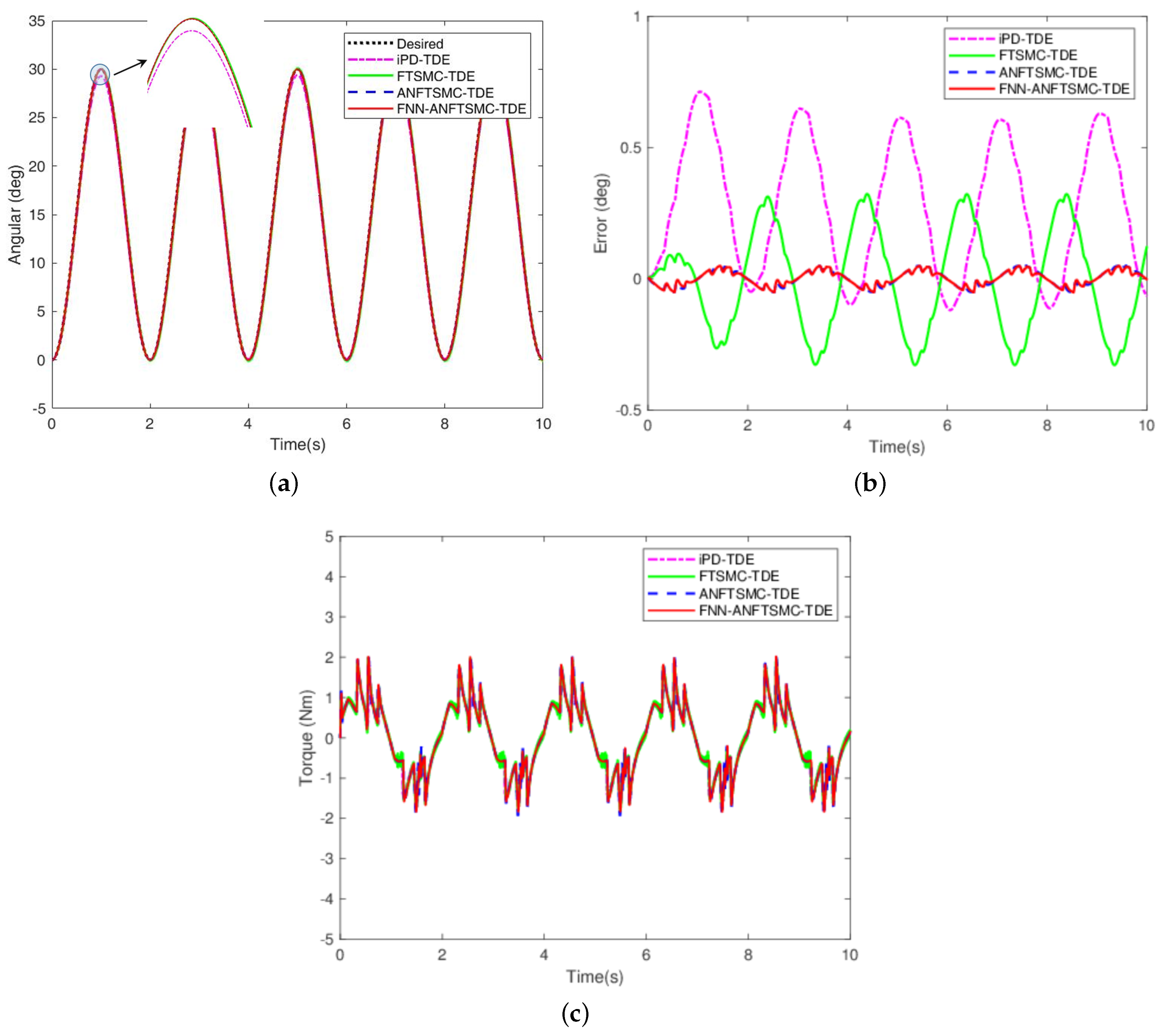
4.4. Simulation Setup

To better clarify the significance of the proposed scheme, the conventional iPD-TDE [44] and FTSMC-TDE [45] algorithms were conducted for comparison. Equations (39) and (40) are referred to as these two existing algorithms, respectively.

$$\begin{array}{cc}\hfill & {\tau }_u=\overline{\mathrm{M}}({\ddot{\theta }}_k+K_D\dot{e}+K_{P}e)+\widehat{F}\left(t\right)\hfill \end{array}$$

(39)

$$\begin{array}{cc}\hfill & s=e+\beta {\dot{e}}^{\frac{m}{n}}\hfill \\ \hfill & {\tau }_u=-\overline{\mathrm{M}}\left({\left(\beta \frac{m}{n}\right)}^{-1}{\dot{e}}^{2-\frac{m}{n}}\right)-\overline{\mathrm{M}}({\gamma }_{1}s+{\gamma }_2{s}^{\frac{n}{m}})+\hfill \\ \hfill & \overline{\mathrm{M}}{\ddot{\theta }}_k+\widehat{F}\left(t\right)\hfill \end{array}$$

(40)

The parameters of the four controllers are listed in

Table 2. The parameters of four controllers.

Parameter (Equation)	iPD-TDE	FTSMC -TDE	ANFTSMC -TDE	FNN- ANFTSMC -TDE
$\overline{\mathrm{M}}$	$0.001$	$0.001$	$0.001$	$0.001$
$K_P$ Equation (39)	$0.05$
$K_D$ Equation (39)	$0.02$
$\beta$ Equation (40)		$0.5$
m Equations (12) and (40)		5	5	5
n Equations (12) and (40)		3	3	3
${\gamma }_1$ Equation (12)		10	1	1
${\gamma }_2$ Equation (12)		1	$0.1$	$0.1$
a Equation (12)			2	2
$\eta$ Equation (17)			20	20
$\sigma$ Equation (25)			$0.01$	$0.01$
c Equation (28)				[$-3$ $-1$ 0 1 3; $-3$ $-1$ 0 1 3]
b Equation (28)				$\left[22222\right]$
$\kappa$ Equation (34)				$0.1$

. They are manually adjusted by trial-and-error.

The APK was to follow the desired trajectory ${\theta }_d=15\ast sin(\pi \ast t-\pi /2)+15$, as depicted in Figure 5 (dashed black line). The initial velocity and acceleration were set to zero. The sampling time T was 0.001 s. The elastic stiffness of the joint was set to 2.1 N/mm. The velocity of the prosthetic knee was calculated by ${\dot{\theta }}_k\left(t\right)=({\theta }_k\left(t\right)-{\theta }_k(t-T))/T$, and the corresponding acceleration could be evaluated as ${\ddot{\theta }}_k\left(t\right)=({\theta }_k\left(t\right)-2{\theta }_k(t-T)+{\theta }_k(t-2T))/T^2$ by numerical differentiation. From the results in Figure 5a–c, it can be concluded that these four TDC schemes can guarantee trajectory tracking under system uncertainties. The validity of the TDE algorithm was proved effectively. Compared with iPD-TDE and FTSMC-TDE, ANFTSMC-TDE and FNN-ANFTSMC-TDE have similar better convergences and the tracking error can be limited in $\left|e\right|<0.051$.

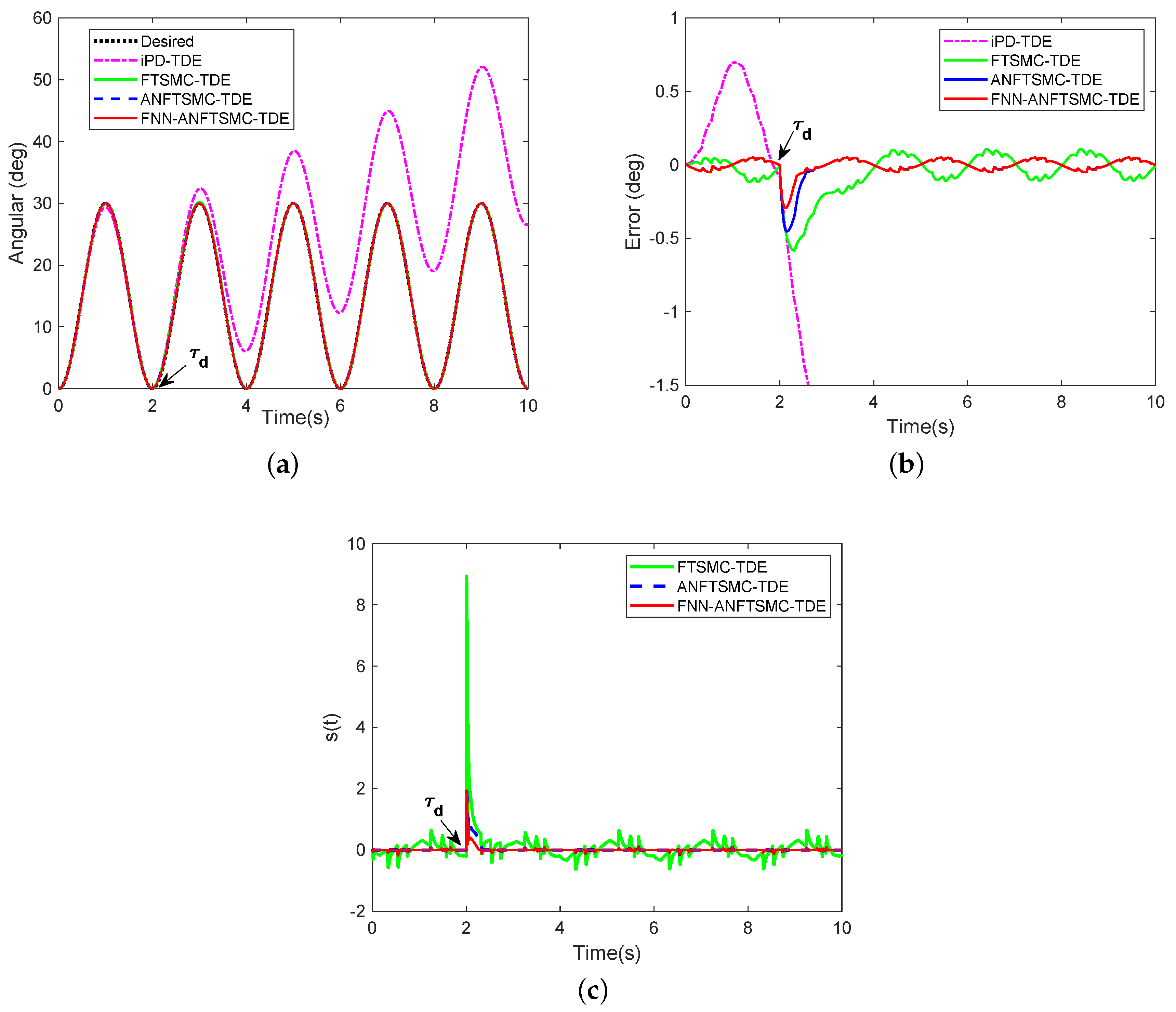
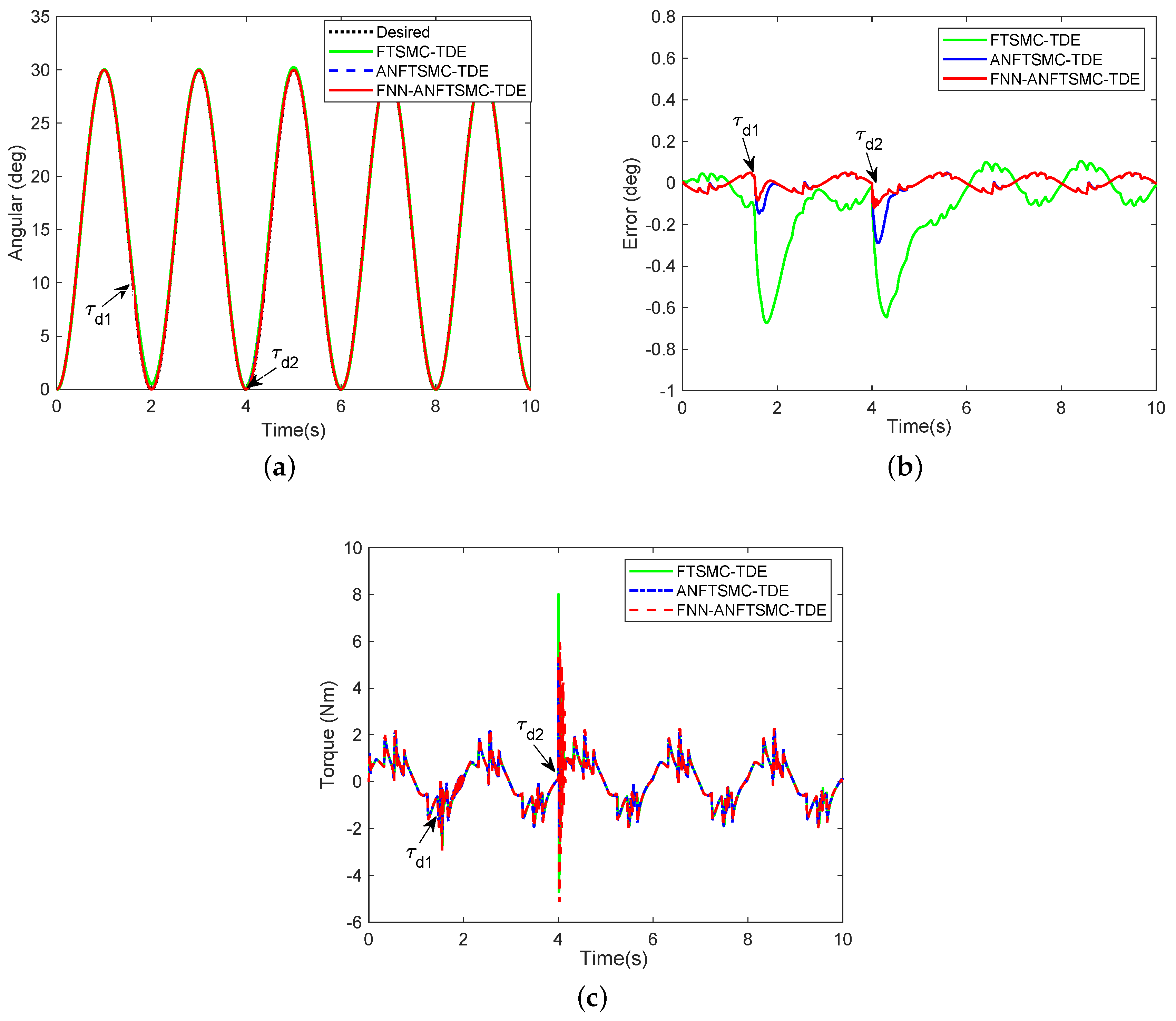
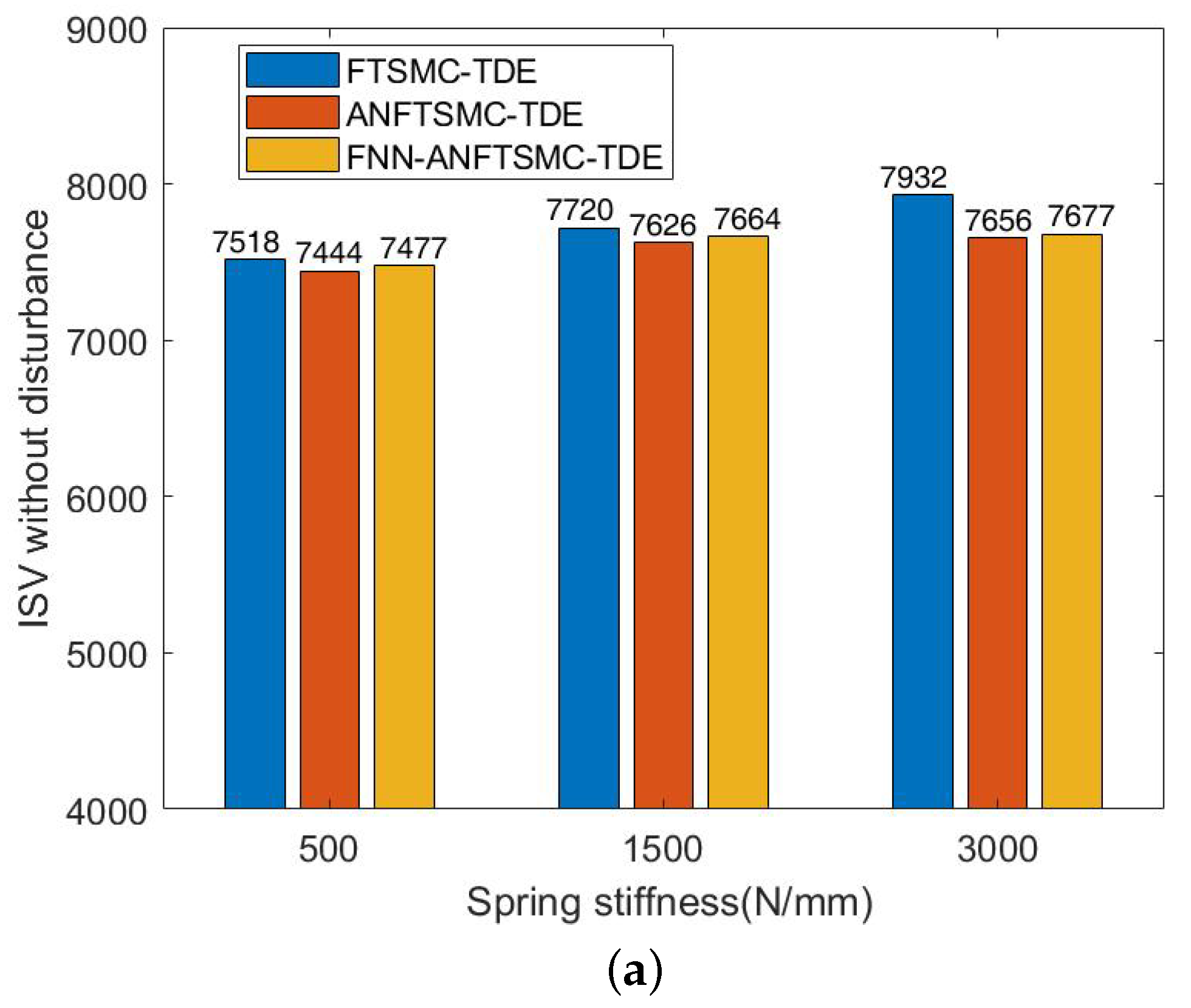
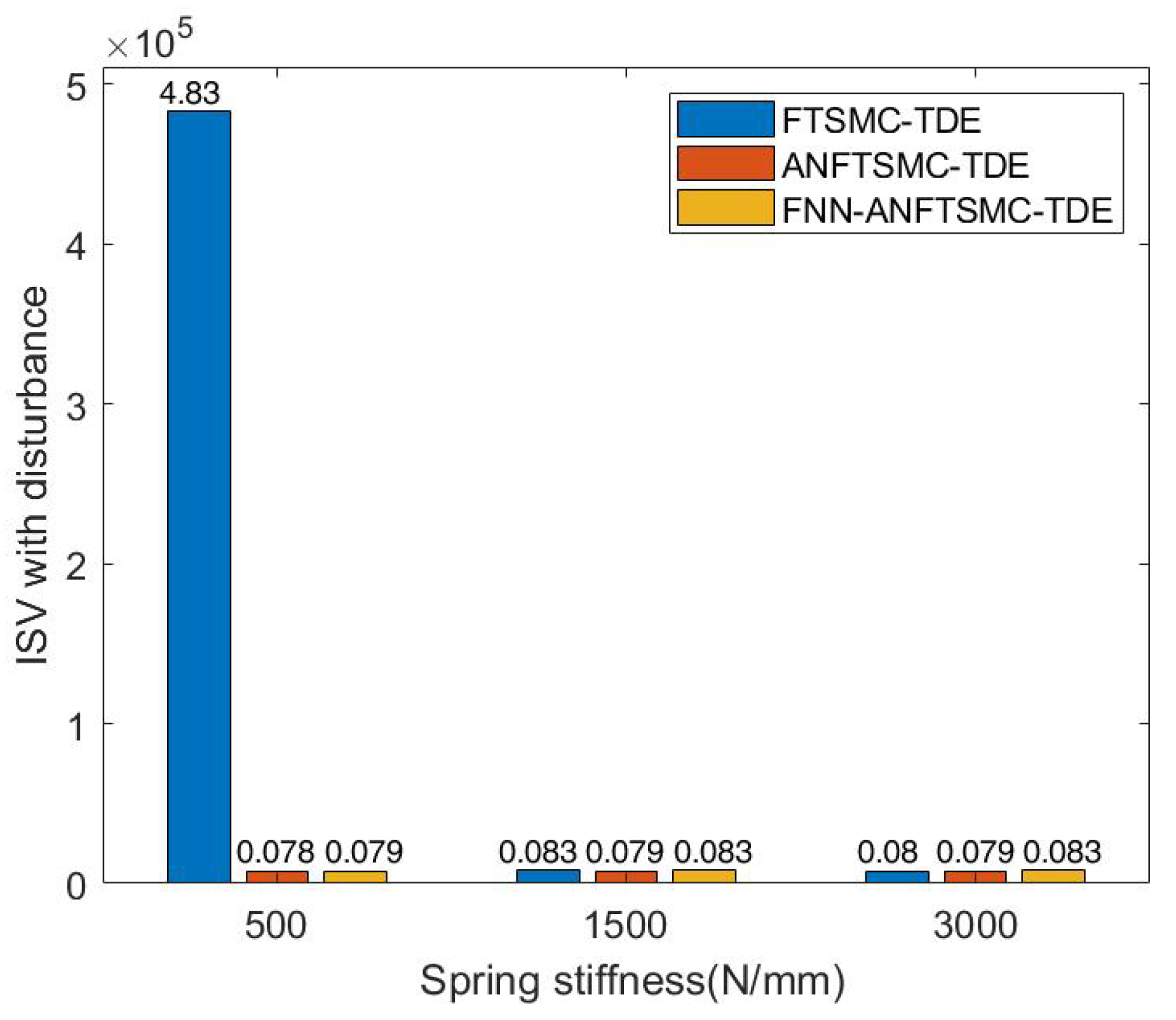
4.5. Robustness Verification

To confirm the robustness of the proposed scheme under uncertain disturbances, ${\tau }_d=7Nm$ was introduced into the knee joint at the time t = 2 s. The angular trajectories in Figure 6a,b show that the disturbance has the greatest influence on the iPD-TDE scheme. The tracking performance of iPD-TDE degrades significantly under the effect of interference. ANFTSMC-TDE and FNN-ANFTSMC-TDE techniques can complete the tracking task with unknown disturbance. It is obvious that the application of FNN makes the system return to a stable state more quickly under interference. Sliding variable s among ANFTSMC-TDE and FNN-ANFTSMC-TDE has converged on the smaller layer, as shown in Figure 6c.

Furthermore, we supplied two more complex disturbances ${\tau }_{d1}=0.5\ast u$ and ${\tau }_{d2}=8\ast q+10\ast {\dot{q}}^2+5\ast cos\left(q\right)$ into the system. The previous disturbance means a $50\%$ loss fault in the actuator at $1.5s$ and the duration was 0.03 s. The latter disturbance is a time-varying signals at t = 4 s. No experiments on iPD-TDE were performed due to failure tracking at any disturbance. To facilitate comparison, based on Figure 7a–c, we can draw the following conclusions: (1) FNN-ANFTSMC-TDE and ANFTSMC-TDE give better performance compared to FTSMC-TDE under all kinds of interference; and (2) FNN-ANFTSMC-TDE has stronger robustness when interference occurs.

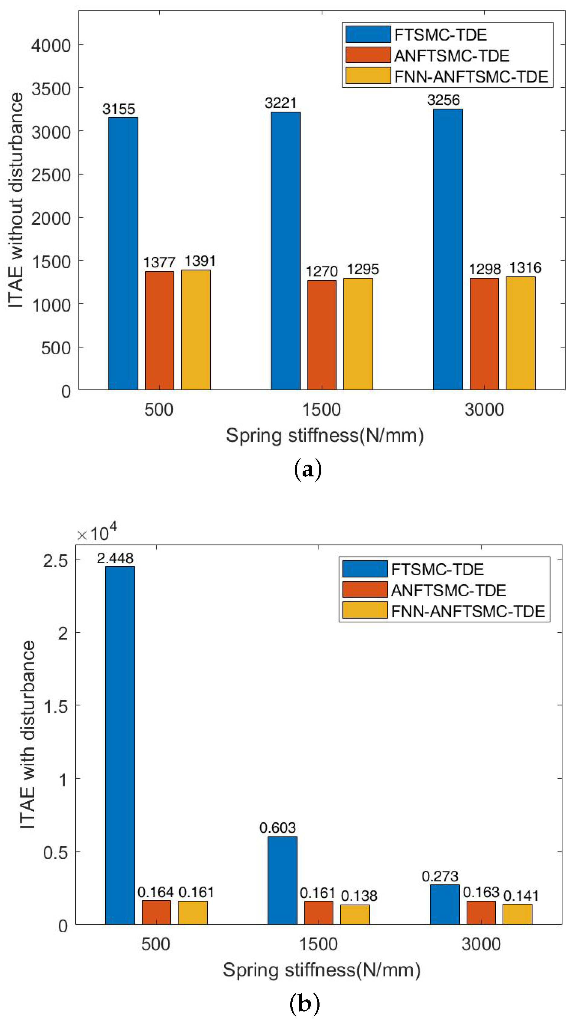
4.6. Performance Analysis

The performance of the three above-mentioned controllers with different joint stiffness were compared. The control performance was evaluated by ITAE and ISV [46]. ITAE represents the cumulative value of tracking error and ISV indicates the energy consumption of the system. Their definitions are as follows:

$$ITAE={\int }_0^{t_s}t\left|e_i\left(t\right)\right|dt$$

(41)

and

$$ISV={\int }_0^{t_s}{\tau }_i^2\left(t\right)dt$$

(42)

We set the stiffness component of APK to 5, 15, and 30 N/mm, respectively. The ITAE and ISV values of the three controllers were compared without disturbance and with disturbances (when ${\tau }_{d1}$ and ${\tau }_{d2}$ occur). The proposed scheme shows better tracking accuracies in Figure 8a,b. Compared with the proposed method, the FTSMC-TDE error increases significantly with the decrease of stiffness under the effect of the same interference signal. From the ISV in Figure 9a,b, the proposed control shows lower energy consumption and the results testify to the energy storage of VSA, which can reduce energy consumption by properly adjusting stiffness.

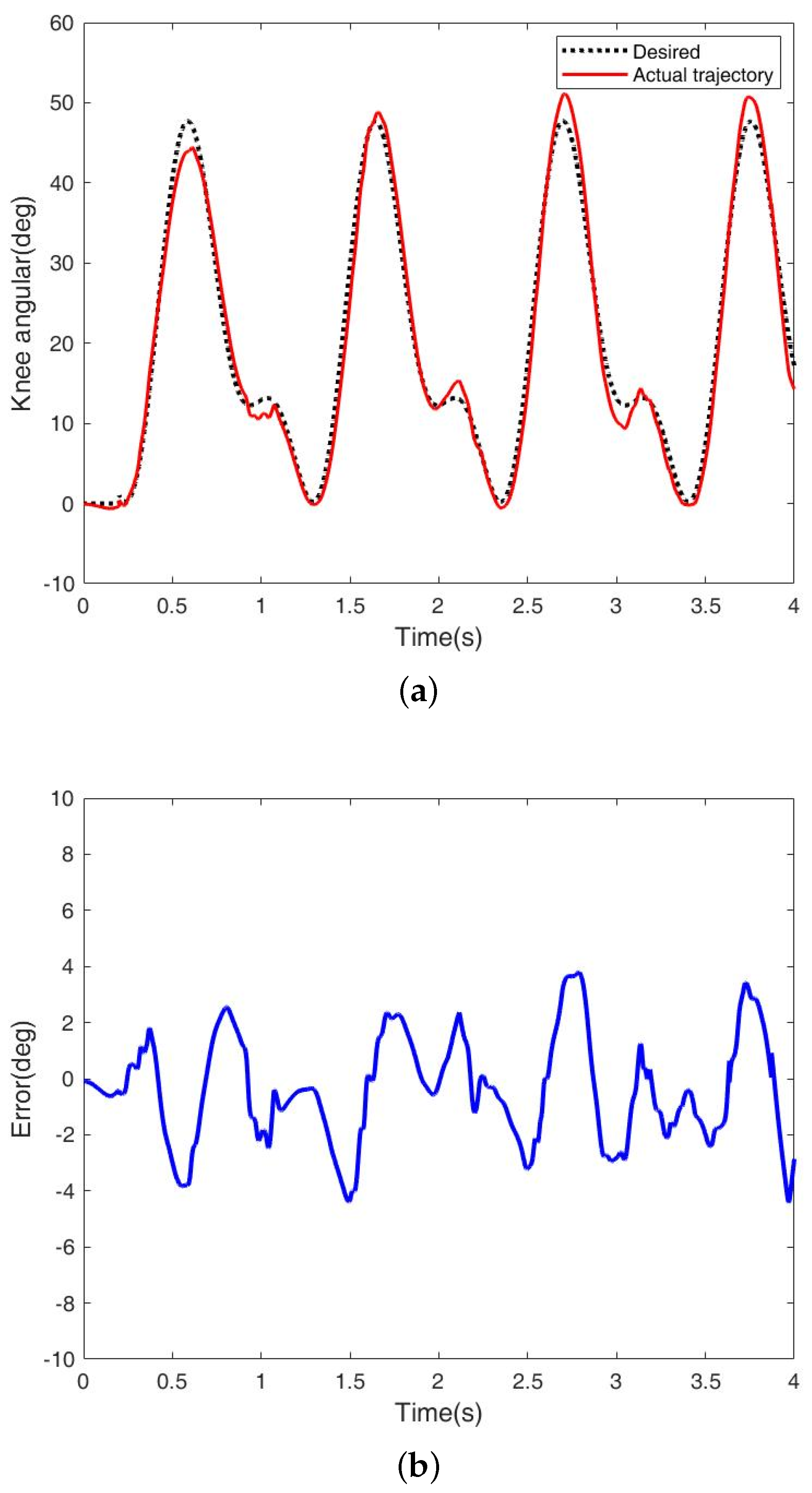
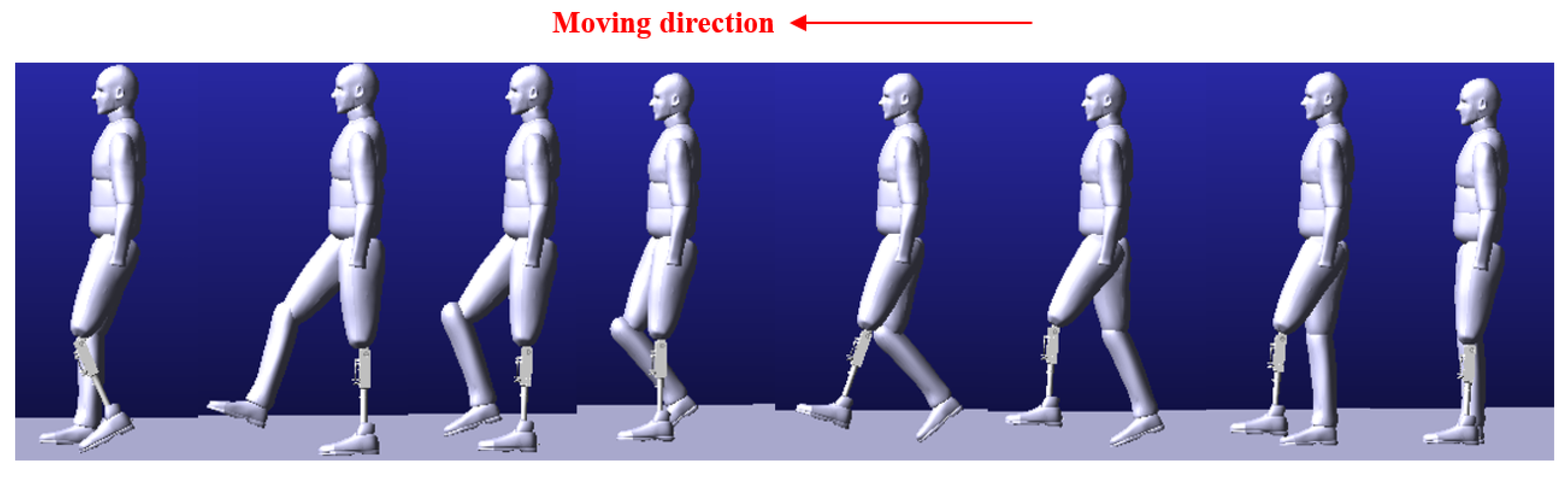
4.7. Human–Machine Hybrid Simulation

For the purpose of the human–machine hybrid approach, the movement data of biological hip and knee joints should be collected by real walking experiments. We used a three-dimensional gait motion capture and training system (GaitWatch) to obtain the lower extremity joint data of the human body whose height is close to that of the model. Three-dimensional gait motion capture and training system (GaitWatch) was used to collect walking data for ten gait cycles, which were used in the double hip joint and right knee joint of the human model. Then, the motion data were added to the motion pair of the two hip joints and right knee joint of the human–machine hybrid model in ADAMS, and the APK was driven by the torque, which was the output of Simulink, that is, the output of the proposed FNN-ANFTSMC-TDE controller.

To further study the application of the adaptive control algorithm in the human–machine hybrid system, a human–machine hybrid model was established in ADAMS. The height of the model is 1.79 m, and the left lower limb is replaced by the APK. To enable the human–machine hybrid virtual model to imitate the walking motion of the human body, it was necessary to input the motion tracking data to the corresponding joints. In addition to the trajectory of the APK controlled by the controller proposed in this paper, the motion trajectory of the other two hip joints and the right knee joint should be directly set in ADAMS. The experimental results are shown in Figure 10 and Figure 11.

It can be concluded from the results in Figure 10 that the gait tracking error of the human–machine hybrid system is more significant than that of the one-leg swing because of various nonlinear and uncertain factors. However, this accuracy is sufficient to ensure humans walk stably. As shown in Figure 11, the dynamic screenshot of a gait cycle is described, and the posture of the prosthetic knee is natural. Gait tracking control is well realized in this paper.

5. Conclusions

In this paper, the design and control method of a variable stiffness actuated APK is proposed. The design of APK is based on previous work on series-elastic actuated robots and is expected to be able to adapt to more complex environments with more flexibility. The control approach is a model-independent control using ANFTSMC and FNN with TDE. To apply this controller to APK, the angular trajectory tracking can be implemented without using an explicit model of the system’s internal dynamics. Numerical simulation validated the effectiveness of this robust adaptive control method. Compared with the existing approach, the proposed scheme has significant improvement in robustness. Simulation results verify that the VSA joint provides the ability to reduce energy consumption while ensuring control accuracy. In future work, to effectively use the energy collection and utilization, we will consider establishing an energy recovery system, collecting the remaining energy during walking, and then rationally distributing and using it. At the same time, benefiting from the theoretical analysis and simulation results, we will also consider how to apply the simulation results to a practical system.

It is worth noting that the scheme proposed in this paper was used to preliminarily verify the controllability and performance of the variable stiffness joint. Meanwhile, the proposed method is currently conformed in the swing phase of APK and the human–machine hybrid virtual model. This work will be the basis for further research. In the future, the gait-based force/position control method will be verified on the prototype of a prosthesis built by the Robot Research Center of Zhongshan institute.

References

1. Zhang, X.; Li, J.; Hu, Z.; Qi, W.; Zhang, L.; Hu, Y.; Su, H.; Ferrigno, G.; Momi, E.D. Novel Design and Lateral Stability Tracking Control of a Four-Wheeled Rollator. Appl. Sci. 2019, 9, 2327. [Google Scholar] [CrossRef] [Green Version]
2. Tucker, M.R.; Olivier, J.; Pagel, A.; Bleuler, H.; Bouri, M.; Lambercy, O.; Millán, J.d.R.; Riener, R.; Vallery, H.; Gassert, R. Control strategies for active lower extremity prosthetics and orthotics: A review. J. NeuroEng. Rehabil. 2015, 12, 1. [Google Scholar] [CrossRef] [Green Version]
3. Li, Z.; Huang, B.; Ajoudani, A.; Yang, C.; Su, C.Y.; Bicchi, A. Asymmetric bimanual control of dual-arm exoskeletons for human-cooperative manipulations. IEEE Trans. Robot. 2017, 34, 264–271. [Google Scholar] [CrossRef]
4. Azimi, V.; Abolfazl Fakoorian, S.; Tien Nguyen, T.; Simon, D. Robust Adaptive Impedance Control With Application to a Transfemoral Prosthesis and Test Robot. J. Dyn. Syst. Meas. Control 2018, 140, 121002. [Google Scholar] [CrossRef] [Green Version]
5. Li, Z.; Huang, B.; Ye, Z.; Deng, M.; Yang, C. Physical Human–Robot Interaction of a Robotic Exoskeleton by Admittance Control. IEEE Trans. Ind. Electron. 2018, 65, 9614–9624. [Google Scholar] [CrossRef] [Green Version]
6. Li, Z.; Yuan, Y.; Luo, L.; Su, W.; Zhao, K.; Xu, C.; Huang, J.; Pi, M. Hybrid brain/muscle signals powered wearable walking exoskeleton enhancing motor ability in climbing stairs activity. IEEE Trans. Med Robot. Bionics 2019, 1, 218–227. [Google Scholar] [CrossRef]
7. Hoover, C.D.; Fulk, G.D.; Fite, K.B. The Design and Initial Experimental Validation of an Active Myoelectric Transfemoral Prosthesis. J. Med. Devices 2012, 6, 011005. [Google Scholar] [CrossRef]
8. Gregg, R.D.; Lenzi, T.; Hargrove, L.J.; Sensinger, J.W. Virtual Constraint Control of a Powered Prosthetic Leg: From Simulation to Experiments With Transfemoral Amputees. IEEE Trans. Robot. 2014, 30, 1455–1471. [Google Scholar] [CrossRef] [Green Version]
9. Li, Z.; Su, C.Y.; Li, G.; Su, H. Fuzzy approximation-based adaptive backstepping control of an exoskeleton for human upper limbs. IEEE Trans. Fuzzy Syst. 2014, 23, 555–566. [Google Scholar] [CrossRef]
10. Sup, F.; Bohara, A.; Goldfarb, M. Design and Control of a Powered Transfemoral Prosthesis. Int. J. Robot. Res. 2008, 27, 263–273. [Google Scholar] [CrossRef] [Green Version]
11. Lawson, B.E.; Mitchell, J.; Truex, D.; Shultz, A.; Ledoux, E.; Goldfarb, M. A Robotic Leg Prosthesis: Design, Control, and Implementation. IEEE Robot. Autom. Mag. 2014, 21, 70–81. [Google Scholar] [CrossRef]
12. Ahn, H.J.; Lee, K.H.; Lee, C.H. Design optimization of a knee joint for an active transfemoral prosthesis for weight reduction. J. Mech. Sci. Technol. 2017, 31, 5905–5913. [Google Scholar] [CrossRef]
13. Martinez-Villalpando, E.C.; Hugh, H. Agonist-antagonist active knee prosthesis: A preliminary study in level-ground walking. J. Rehabil. Res. Dev. 2009, 46, 361–373. [Google Scholar] [CrossRef]
14. Rouse, E.J.; Mooney, L.M.; Herr, H.M. Clutchable series-elastic actuator: Implications for prosthetic knee design. Int. J. Robot. Res. 2014, 33, 1611–1625. [Google Scholar] [CrossRef]
15. Geeroms, J.; Flynn, L.; Jimenez-Fabian, R.; Vanderborght, B.; Lefeber, D. Design and energetic evaluation of a prosthetic knee joint actuator with a lockable parallel spring. Bioinspir. Biomimetics 2017, 12, 026002. [Google Scholar] [CrossRef]
16. Zhang, X.; Li, J.; Fan, K.; Chen, Z.; Hu, Z.; Yu, Y. Neural Approximation Enhanced Predictive Tracking Control of a Novel Designed Four-Wheeled Rollator. Appl. Sci. 2020, 10, 125. [Google Scholar] [CrossRef] [Green Version]
17. Su, H.; Yang, C.; Mdeihly, H.; Rizzo, A.; Ferrigno, G.; De Momi, E. Neural Network Enhanced Robot Tool Identification and Calibration for Bilateral Teleoperation. IEEE Access 2019, 7, 122041–122051. [Google Scholar] [CrossRef]
18. Zhang, X.; Li, J.; Ovur, S.E.; Chen, Z.; Li, X.; Hu, Z.; Hu, Y. Novel Design and Adaptive Fuzzy Control of a Lower-Limb Elderly Rehabilitation. Electronics 2020, 9, 343. [Google Scholar] [CrossRef] [Green Version]
19. Stoeffler, C.; Kumar, S.; Peters, H.; Brüls, O.; Müller, A.; Kirchner, F. Conceptual Design of a Variable Stiffness Mechanism in a Humanoid Ankle using Parallel Redundant Actuation. In Proceedings of the 2018 IEEE-RAS 18th International Conference on Humanoid Robots (Humanoids), Beijing, China, 6–9 November 2018; pp. 462–468. [Google Scholar]
20. Wang, B.; Wang, J.; Wang, S.; Li, J. Parallel Structure of Six Wheel-legged Robot Model Predictive Tracking Control based on Dynamic Model. In Proceedings of the 2019 Chinese Automation Congress (CAC), Hangzhou, China, 22–24 November 2019; pp. 5143–5148. [Google Scholar]
21. Liu, Z.; Lin, W.; Geng, Y.; Yang, P. Intent pattern recognition of lower-limb motion based on mechanical sensors. IEEE/CAA J. Autom. Sin. 2017, 4, 651–660. [Google Scholar] [CrossRef]
22. Peng, F.; Peng, W.; Zhang, C.; Zhong, D. IoT Assisted Kernel Linear Discriminant Analysis Based Gait Phase Detection Algorithm for Walking with Cognitive Tasks. IEEE Access 2019, 7, 68240–68249. [Google Scholar] [CrossRef]
23. Qi, W.; Su, H.; Yang, C.; Ferrigno, G.; De Momi, E.; Aliverti, A. A Fast and Robust Deep Convolutional Neural Networks for Complex Human Activity Recognition Using Smartphone. Sensors 2019, 19, 3731. [Google Scholar] [CrossRef] [Green Version]
24. Su, H.; Qi, W.; Hu, Y.; Sandoval, J.; Zhang, L.; Schmirander, Y.; Chen, G.; Aliverti, A.; Knoll, A.; Ferrigno, G.; et al. Towards Model-Free Tool Dynamic Identification and Calibration Using Multi-Layer Neural Network. Sensors 2019, 19, 3636. [Google Scholar] [CrossRef] [Green Version]
25. Youcef-Toumi, K.; Ito, O. A Time Delay Controller for Systems with Unknown Dynamics. In Proceedings of the 1988 American Control Conference, Atlanta, GA, USA, 15–17 June 1988; pp. 904–913. [Google Scholar]
26. Jin, M.; Lee, J.; Tsagarakis, N.G. Model-Free Robust Adaptive Control of Humanoid Robots with Flexible Joints. IEEE Trans. Ind. Electron. 2017, 64, 1706–1715. [Google Scholar] [CrossRef]
27. Li, Z.; Li, J.; Zhao, S.; Yuan, Y.; Kang, Y.; Chen, C.P. Adaptive neural control of a kinematically redundant exoskeleton robot using brain-machine interfaces. IEEE Trans. Neural Networks Learn. Syst. 2018, 30, 3558–3571. [Google Scholar] [CrossRef]
28. Jin, M.; Lee, J.; Chang, P.H.; Choi, C. Practical Nonsingular Terminal Sliding-Mode Control of Robot Manipulators for High-Accuracy Tracking Control. IEEE Trans. Ind. Electron. 2009, 56, 3593–3601. [Google Scholar]
29. Van, M.; Ge, S.S.; Ren, H. Finite Time Fault Tolerant Control for Robot Manipulators Using Time Delay Estimation and Continuous Nonsingular Fast Terminal Sliding Mode Control. IEEE Trans. Cybern. 2017, 47, 1681–1693. [Google Scholar] [CrossRef]
30. Su, H.; Qi, W.; Yang, C.; Aliverti, A.; Ferrigno, G.; De Momi, E. Deep Neural Network approach in Human-Like Redundancy Optimization for Anthropomorphic Manipulators. IEEE Access 2019, 7, 124207–124216. [Google Scholar] [CrossRef]
31. Su, H.; Ovur, S.E.; Zhou, X.; Qi, W.; Ferrigno, G.; De Momi, E. Depth vision guided hand gesture recognition using electromyographic signals. Adv. Robot. 2020, 1–13. [Google Scholar] [CrossRef]
32. Chang, J.L. Sliding mode control design for mismatched uncertain systems using output feedback. Int. J. Control. Autom. Syst. 2016, 14, 579–586. [Google Scholar] [CrossRef]
33. Wang, Y.; Chen, J.; Zhu, K.; Chen, B.; Wu, H. Time-Delay Control of Cable-Driven Robots with Adaptive Fractional-Order Nonsingular Terminal Sliding Mode. IEEE Access 2018, 6, 54086–54096. [Google Scholar] [CrossRef]
34. Ham, R.V.; Sugar, T.G.; Vanderborght, B.; Hollander, K.W.; Lefeber, D. Compliant actuator designs. IEEE Robot. Autom. Mag. 2009, 16, 81–94. [Google Scholar] [CrossRef]
35. Li, X.; Pan, Y.; Chen, G.; Yu, H. Multi-modal control scheme for rehabilitation robotic exoskeletons. Int. J. Robot. Res. 2017, 36, 759–777. [Google Scholar] [CrossRef]
36. Liang, P.; Yang, C.; Wang, N.; Li, Z.; Li, R.; Burdet, E. Implementation and Test of Human-Operated and Human-Like Adaptive Impedance Controls on Baxter Robot; Advances in Autonomous Robotics Systems; Springer International Publishing: Cham, Switzerland, 2014; pp. 109–119. [Google Scholar]
37. Veneman, J.F.; Ekkelenkamp, R.; Kruidhof, R.; van der Helm, F.C.; van der Kooij, H. A Series Elastic- and Bowden-Cable-Based Actuation System for Use as Torque Actuator in Exoskeleton-Type Robots. Int. J. Robot. Res. 2006, 25, 261–281. [Google Scholar] [CrossRef]
38. Wolf, S.; Hirzinger, G. A new variable stiffness design: Matching requirements of the next robot generation. In Proceedings of the 2008 IEEE International Conference on Robotics and Automation, Pasadena, CA, USA, 19–23 May 2008; pp. 1741–1746. [Google Scholar]
39. Li, Z.; Xu, C.; Wei, Q.; Shi, C.; Su, C.Y. Human-Inspired Control of Dual-Arm Exoskeleton Robots with Force and Impedance Adaptation. IEEE Trans. Syst. Man Cybern. Syst. 2018. [Google Scholar] [CrossRef]
40. Precup, R.E.; Radac, M.B.; Roman, R.C.; Petriu, E.M. Model-free sliding mode control of nonlinear systems: Algorithms and experiments. Inf. Sci. 2017, 381, 176–192. [Google Scholar] [CrossRef]
41. Yang, L.; Yang, J. Nonsingular fast terminal sliding-mode control for nonlinear dynamical systems. Int. J. Robust Nonlinear Control 2011, 21, 1865–1879. [Google Scholar] [CrossRef]
42. Lee, J.; Chang, P.H.; Jin, M. Adaptive Integral Sliding Mode Control With Time-Delay Estimation for Robot Manipulators. IEEE Trans. Ind. Electron. 2017, 64, 6796–6804. [Google Scholar] [CrossRef]
43. Rouhani, E.; Erfanian, A. A Finite-time Adaptive Fuzzy Terminal Sliding Mode Control for Uncertain Nonlinear Systems. Int. J. Control. Autom. Syst. 2018, 16, 1938–1950. [Google Scholar] [CrossRef]
44. Fliess, M.; Join, C. Model-free control. Int. J. Control 2013, 86, 2228–2252. [Google Scholar] [CrossRef] [Green Version]
45. Jin, M.; Lee, J.; Ahn, K.K. Continuous Nonsingular Terminal Sliding-Mode Control of Shape Memory Alloy Actuators Using Time Delay Estimation. IEEE/ASME Trans. Mechatronics 2015, 20, 899–909. [Google Scholar] [CrossRef]
46. Viveiros, C.; Melicio, R.; Igreja, J.; Mendes, V. Performance Assessment of a Wind Turbine Using Benchmark Model: Fuzzy Controllers and Discrete Adaptive LQG. Procedia Technol. 2014, 17, 487–494. [Google Scholar] [CrossRef] [Green Version]
Figure 1. Mechanical structure of APK: (a) the mechanical structure of the VSA joint; (b) virtual prototype; and (c) physical prototype.
Applsci 10 02755 g001
Figure 2. The diagram of a human–machine hybrid system in sagittal plane.
Applsci 10 02755 g002
Figure 3. The schematic diagram of the VSA-Joint.
Applsci 10 02755 g003
Figure 4. Block diagram of FNN-ANFTSMC-TDE.
Applsci 10 02755 g004
Figure 5. Simulation results of comparison among iPD-TDE, FTSMC-TDE, ANFTSMC-TDE, and FNN-ANFTSMC-TDE: (a) trajectory tracking; (b) trajectory error; and (c) control torque.
Applsci 10 02755 g005
Figure 6. Simulation results of comparison among iPD-TDE, FTSMC-TDE, ANFTSMC-TDE, and FNN-ANFTSMC-TDE when τ d ( t = 2 s) occurs: (a) trajectory tracking with τ d ; (b) trajectory error with τ d ; and (c) sliding surface with τ d .
Applsci 10 02755 g006
Figure 7. Simulation results of comparison among FTSMC-TDE, ANFTSMC-TDE, and FNN-ANFTSMC-TDE when τ d 1 ( t = 1.5 s) and τ d 2 ( t = 4 s) occur: (a) trajectory tracking with τ d 1 and τ d 2 ; (b) trajectory error with τ d 1 and τ d 2 ; and (c) control torque with τ d 1 and τ d 2 .
Applsci 10 02755 g007
Figure 8. Simulation results of ITAE among FTSMC-TDE, ANFTSMC-TDE, and FNN-ANFTSMC-TDE under different joint stiffnesses: (a) ITAE without disturbance; and (b) ITAE when τ d 1 and τ d 2 occur.
Applsci 10 02755 g008
Figure 9. Simulation results of ISV among FTSMC-TDE, ANFTSMC-TDE, and FNN-ANFTSMC-TDE under different joint stiffnesses: (a) ISV without disturbance; and (b) ISV when τ d 1 and τ d 2 occur.
Applsci 10 02755 g009aApplsci 10 02755 g009b
Figure 10. Trajectory tracking of the APK in man–machine hybrid model: (a) knee angular tracking; and (b) tracking error.
Applsci 10 02755 g010
Figure 11. A gait cycle dynamic screenshot of the human–machine hybrid model.
Applsci 10 02755 g011