Abstract
Bearing preload significantly affects the running performance of a shaft-bearing system including the fatigue life, wear, and stiffness. Due to the mounting error, the bearing rings are often angularly misaligned. The effects of the combined bearing preload and angular misalignment on the fatigue life of ball bearings and a shaft-bearing system are analyzed in this paper. The contact force distribution of angular contact ball bearings in the shaft-bearing system is investigated based on the system model. The system model includes the bearing model, and the shaft model is verified by comparing with the manufacturer’s manual and the results from other theoretical models, with the difference between the results from the present bearing model and manufacturer manual within 3%. The global optimization method is used to replace the Newton–Raphson algorithm to solve the ball elements’ displacements and friction coefficients, which improves the computation efficiency of the system model. The fatigue life of each bearing is evaluated with the consideration of the two preload methods and two angular misalignment cases. The fatigue life results show that the system life at the optimal angular misalignment is more than 1.5 times that without angular misalignment at the low preload value, and this ratio decreases as the preload value increases. The optimal angular misalignment of both the shaft-bearing system and the misaligned bearing is not always consistent, which depends on the preload value and bearing life. Both the constant-displacement preload and constant-force preload do not cause a significant difference in the highest system life. The different misaligned bearings can lead to different highest system lives as the preload value is low.
1. Introduction
The shaft-bearing system is a key part in mechanical transmissions, in which the rolling element bearing is commonly applied due to its low friction, low wear, and low energy consumption. With the high speed and high precision requirements for rotating machinery, the shaft is usually designed to be supported by multiple rolling element bearings. Many scholars have investigated the dynamic characteristics of the shaft-bearing system [1,2,3], and a comprehensive review on dynamic model development of a shaft-bearing system was also presented [4]. In addition to dynamic analysis, the fatigue life of both the rolling element bearing and shaft system has also attracted much attention. Among various causes that affect the fatigue life of the rolling element bearing, both preload and angular misalignment are two common and important factors.
Many researchers have conducted numerous studies on the fatigue life of the rolling element bearings considering the preload and angular misalignment. Harris [5], as one of first researchers, presented the dependence of the fatigue life of a cylindrical roller bearing having crowned rolling elements on the angular misalignment. Hagiu [6] investigated the relation between the preload and service life for an angular contact ball bearing by theoretical and experimental methods. Hwang and Lee [7] reviewed the three categories of preload technologies and clarified that the determination of proper preload should take the fatigue life, stiffness, and temperature of rolling element bearings into account. Considering the significance of the pressure distribution of roller elements on the fatigue life estimation, Tong et al. [8] extended the 3D elastic contact method to simulate the contact pressure and analyzed the fatigue life of a tapered roller bearing with the consideration of the angular misalignment effect. Yang et al. [9] analyzed the effects of the combined external loads and angular misalignment on the double-row tapered roller bearing, and the results demonstrated that the external load, rotation speed, and angular misalignment had a significant influence on the fatigue life of a double-row tapered roller bearing. Warda et al. [10,11] investigated the effect of the correction parameters of roller generators and angular misalignment on the fatigue life of the radial cylindrical roller bearing, in which the bearing radial clearance and complex loads were both taken into account.
The above research works were mainly limited to a single bearing, and many works investigated the relations among the preload, fatigue life, temperature, and stiffness in a shaft-bearing system. Jiang et al. [12] investigated a variable preload technology for machine tool spindles working at different ranges of rotation speed, and the experimental results showed that the variable preload technology can reduce the temperature rise of the system in the high speed condition compared with the application of constant preload and improved the bearing stiffness at the low speed range. Xu et al. [13] developed an analytical method for determining the optimum preload based on the critical state between the skidding and rolling of ball bearings for different speed ranges, and their results were verified with the help of a spindle bearing experimental setup. Than and Huang [14] investigated the thermal effect of the spindle bearing system during high speed rotations when the preload was applied, and the time-varying thermal effects on the preload and stiffness of bearings was obtained. Zhang et al. [15] investigated the effect of external load and preload on the number of rolling elements in the contact zone based on the a quasi-dynamic model and determined an optimum preload for a simplified bearing-rotor system by taking the bearing fatigue life as the optimization target.
For the shaft-bearing system with high speed and high precision requirements, bearing preload is necessary to increase bearing stiffness and suppress vibration. In addition, the angular misalignment of the rolling bearing due to mounting error is common and unavoidable and would cause considerable variations in ball-raceways’ contact force distribution, which affects the bearing fatigue life. Currently, very few studies have investigated the effects of the combined preload and angular misalignment on the fatigue life of rolling element bearings and the shaft-bearing system at high speed. The fatigue life variation of rolling element bearings and the shaft-bearing system with the combined preload and angular misalignment has not been well understood. In this sense, understanding the fatigue life variation considering the combined preload and angular misalignment is important for proper selection and assembly of rolling bearings in the shaft-bearing system, which can be achieved by analyzing the effects of the combined preload and angular misalignment on the fatigue life of rolling element bearings and the shaft-bearing system.
In this paper, a generic shaft-bearing system model combing the shaft model and the bearing model is introduced. A numerical method is presented to improve the computation efficiency of the system model. The ball-raceway contact forces of angular contact ball bearings (ACBBs) in shaft-bearing systems are evaluated under the complex operation conditions considering both the preload and angular misalignment. Based on the fatigue life theory, the fatigue life of each ACBB is calculated. The effects of the combined preload and angular misalignment on the fatigue life of ACBBs and the shaft-bearing system are discussed. Finally, some useful conclusions are given.
2. Shaft-Bearing System Model
2.1. Quasi-Static Model of Angular Contact Ball Bearing
The scheme diagram of a shaft supported by multiple ACBBs is shown in Figure 1. O-xyz denotes the inertial coordinate system where the z-axis is coincident with the shaft axis, and Ok-xkykzk denotes the local coordinate system for the kth bearing in which the forward direction of the zk-axis is defined as from the small side of the bearing to its big side. Here, the quasi-static bearing model is presented in the bearing local coordinate system. A ball bearing is taken as an example to analyze the interactions between ball elements and raceways.
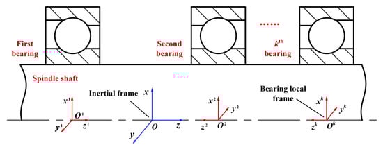
Figure 1.
Geometrical configuration of a shaft-bearing system.
The kinematics of the ball element is shown in Figure 2. Here, the inner ring is assembled with a shaft that rotates at angular speed about the bearing axis while the outer ring is fixed. For a bearing with pitch diameter and ball diameter , one can get the angular speed at which the ball element orbits around the bearing axis and the spinning speed at which the ball element rotates around its own axis as given in Equations (1) and (2), respectively.
where and are the contact angles between the ball and inner/outer raceway. and are equal to and , respectively. is the ball pitch angle.
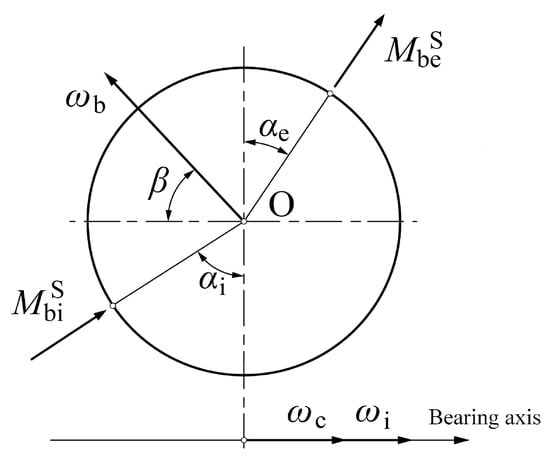
Figure 2.
Kinematic relation of a ball element.
Based on d’Alembert’s inertia force principle, Ding [16] derived the following pitch angle formula as shown in Equation (3).
in which is equal to , and are the friction moments for the ball and inner/outer raceways, respectively, and:
where and are the contact forces between the ball and inner/outer raceway. and are the semi-major axes of the contact ellipses for the ball and inner/outer raceways, respectively. is the second kind of elliptic integral function. and are the ratios of the semi-major axis to the semi-minor axis of the contact ellipses at the ball inner and ball outer raceway contacts, respectively. The detailed derivation of the pitch angle is omitted here and can be found in Ding’s work [16].
The contact angle and contact elastic deformation between the ball element and raceways are shown in Figure 3. When the external loads are applied on the static bearing, the ball center and raceway groove curvature center , are collinear. These three points are no longer collinear due to the centrifugal force of the ball element when the rotating speed is imposed. The ball center will be shifted from to , and the inner raceway groove curvature center moves from to , while the groove curvature center of the outer raceway remains unchanged since the outer ring is fixed.
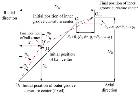
Figure 3.
Positions of ball centers and raceway groove curvature centers.
In Figure 3, , denote the axial and radial distance between the inner and outer raceway groove curvature centers at the jth ball element position and can be written as:
where , , and are the translational displacements of the inner ring along the x-, y-, and z-axis, respectively, and are the angular displacements around the x- and y-axis, respectively. is the bearing initial contact angle. and are the inner and outer raceway groove curvature coefficients, respectively. The radius of the locus of the inner raceway groove curvature centers and the jth ball element azimuth angle are determined by:
where is the ball element number in the bearing. The loaded contact angles and at ball-raceway contacts can be obtained:
The contact elastic deformations and can be given as:
where and are the axial and radial distances between ball center and outer raceway groove curvature center , respectively.
As shown in Figure 4, considering the centrifugal force , gyroscopic moment , contact forces and , and friction forces and , the force and moment equilibrium equations for the jth ball element can be presented as:
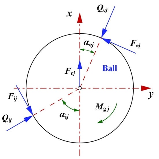
Figure 4.
Forces on the ball element.
Here, an approximate relation between friction forces , and contact forces , , at ball-raceway contacts is applied, as follows:
where is the friction coefficients at ball-raceway contacts.
The centrifugal force and gyroscopic moment for the jth ball element can be written, respectively, as follows:
where is the mass of the ball element and is the mass moment of inertia:
Based on Hertz’s work, the ball-raceway contact forces can be related to the elastic contact deformation presented in Equations (11) and (12).
in which , are the contact stiffness coefficients and can be calculated based on Harris and Kotzalas’ work [17].
The bearing loads applied on the inner ring from the shaft include the translational forces , , and and moments , . The total bearing loads should be balanced by contact forces and friction forces between ball elements and the inner raceway, and the equilibrium relations of the inner ring can be presented as:
in which is the groove curvature radius of the inner raceway.
2.2. Shaft Model
In order to consider shaft flexibility, the finite element method is adopted here, and the shaft is discretized into segments containing nodes using Timoshenko’s beam element, as shown in Figure 5. O-xyz is the inertial coordinate system of the whole shaft-bearing system (mentioned in Section 2.1). The torsional deformation of the shaft is ignored; only the bending and axial deformations are considered. The ith node on beam element has three translational DOFs , , and along the x-, y-, and z-axis, respectively, and two rotational DOFs , around the x- and y-axis, respectively. In the present shaft-bearing system, the bearing inner ring is close fit with the shaft; therefore, the inner ring of the bearing has the same displacements as the shaft node at the bearing mounting position. The displacement vector at the ith node location is:
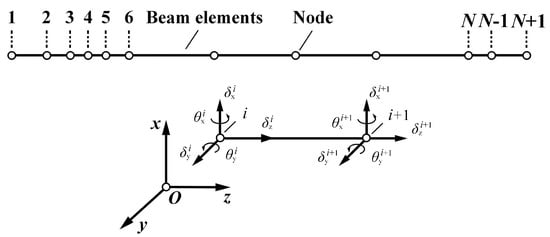
Figure 5.
Finite element model for the shaft.
The corresponding load vector is:
The stiffness matrix for each beam element can be obtained as follows:
where is a parameter including the transverse shear effect of beam, and its detailed expression can be found in [18].
The finite element equilibrium equation of the shaft can be written as:
where is the global stiffness matrix obtained by assembling all the beam element stiffness matrix , is the node displacement vector of the shaft and can be expressed as , and is the load vector applied on the shaft nodes given as . The load vector consists of two parts: one part is attributed to the external loads, and the other part is the supporting loads provided by the ball bearings and also the counter force of the bearing loads calculated in Equation (21). Based on the transformation relation between the bearing local coordinate system and the global inertial coordinate system, the displacements of the bearing inner ring in the bearing local coordinate system can be easily represented by the node displacements of the shaft in the inertial coordinate system at the location where the shaft is supported by the ball bearing. Therefore, the supporting loads applied on the shaft nodes provided by the ball bearings can be expressed as a nonlinear function of the node displacements of the shaft.
2.3. Preload and Angular Misalignment Factors
In the current analysis, the ball bearing is preloaded axially on the outer ring including constant-displacement preload and constant-force preload. The angular misalignment taken into account here is caused by mounting error, and the misaligned inner and outer rings due to mounting error can both lead to angular misalignment. In order to simplify the analysis, the inner ring is assumed to be mounted accurately. The outer ring is misaligned, and its misalignment angle keeps constant when the shaft-bearing is loaded.
Axial preload and angular misalignment can lead to additional deformation in each ball element and cause ball element-raceway contact forces to be redistributed; therefore, they should be included in the calculation of ball element deformation to reflect their effects on the fatigue life. Both the axial preload and angular misalignment affect mainly the axial distance between inner and outer raceway groove curvature centers at the jth ball element position. The translational displacement should be replaced by in Equation (5) to calculate the axial distance when the axial preload is taken into account. The axial displacement is caused by axial preload on the outer ring, which is known when constant-displacement preload is applied and unknown if constant-force preload is applied. When angular misalignment components of the outer ring of the ball bearing, and , are considered, the angular displacements and should be replaced with and in Equation (5), respectively. Then, the axial distance considering axial preload should be rewritten as:
The axial distance considering the angular misalignment is:
3. Numerical Solution and Model Validity
3.1. Numerical Solution of the System Model
By combining the shaft model and quasi-static model of ACBB, the generic shaft-bearing system model is obtained. The unknowns in the system model include the ball orbital speed , spinning speed , pitch angle , axial and radial distances to imply the final position of the ball center, friction coefficients at ball-raceway contacts, inner ring displacements for ACBB, and the node displacements for the shaft. The unknowns are for each ball bearing and for the shaft. Considering that the inner ring displacements of ball bearings are the same as the displacements of shaft nodes where ball bearings are mounted, the total unknowns of the shaft-bearing system model are , and is the number of ACBBs supporting the shaft. Obviously, the shaft-bearing system model is a huge system of equations provided that the shaft is supported by several ACBBs and the number of ball elements for each bearing and of the beam elements for the shaft is large.
It is computationally infeasible to solve all the equations of the shaft-bearing system model together. Hence, a numerical scheme is proposed to solve the system model. The numerical solution process is presented in Figure 6. The shaft-bearing system properties, including material properties, geometrical parameters, operation conditions, load conditions, axial preload, and/or angular misalignment of ball bearing, are taken as the input parameters. The initial guess for the node displacements of the shaft, the spinning speed , orbital speed , and pitch angle of each ball element are also necessary to start the solution. Then, the distances parameters and friction coefficients of all ball elements in the kth ball bearing are solved together by the global optimization method. The new spinning speed , orbital speed , and pitch angle for ball elements are calculated based on Equations (1)–(3). The distances parameters , friction coefficients , speed parameters (,), and pitch angle are solved alternately until the corresponding converge criterion is reached. Once the above calculations for all the ball bearings are finished, the equilibrium equations of the shaft are checked. Since the loads applied on the shaft nodes provided by the ball bearings are a nonlinear function of the node displacements of the shaft, the equilibrium equation of the shaft, Equation (25), is nonlinear as a function of the shaft nodes’ displacements. Based on the first order Taylor expansion of nonlinear equilibrium equations of the shaft, the node displacements on the shaft are updated. The whole calculation process will be continued until the equilibrium equations of the shaft are satisfied. Then, the node displacements of the shaft, ball-raceway contact forces, spinning speed, orbital speed, and pitch angle for each ball element can be obtained. It should be noted that, in the innermost loop of the flowchart, the Newton–Raphson algorithm is not used to solve the equilibrium Equation (13) of all ball elements simultaneously to obtain the distance parameters and friction coefficients for the kth ball bearing, although this method was commonly used in the previously published works. The accuracy of the Newton–Raphson algorithm typically relies on the trial-and-error of initial estimates, and the numerical scheme will be very time-consuming and not be able to converge if the initial chosen solution is far away from the exact solution. In order to overcome this deficiency, the global optimization method is used to calculate the unknowns and of all ball elements simultaneously for the kth ball bearing. In the global optimization method, the sum of the square of 3Z mathematical formulas at the left of the equilibrium equations Equation (13) of all ball elements in the kth ball bearing is the objective function, and the aim is to find the correct and that make the objective function almost zero (global minimum). The scatter search [19] algorithm is used to generate trial points (initial estimates of independent variables and ). The two filter conditions, the distance filter and merit filter [20], are used to examine trial points to ensure that the trial points that do not actually contribute to finding the local minimum of the objective function are excluded. After examination, the correct and of ball elements can be calculated, which make the objective function nearly zero (global minimum). The calculation shows that the global optimization method is very fast and reliable, and the computational efficiency of the system model is improved significantly.
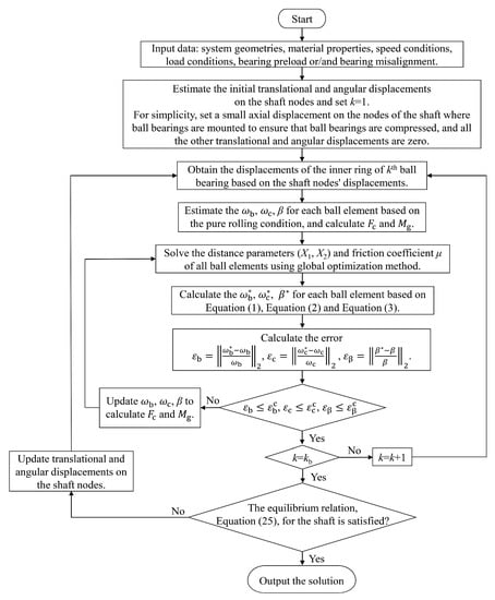
Figure 6.
Flowchart of solving the shaft-bearing system.
3.2. Model Validity
In order to illustrate the validity of the ball bearing model, the contact angle results for the b218 bearing considering different load and speed conditions are compared in Figure 7 with that from Antoine’s work [21]. It can be seen that the contact angle obtained by the present ball bearing model agreed well with the previously published results, and the maximum relative error between them was 16% as the preload was near 8000 N and the bearing speed was 10,000 rpm; However, the error was very small for other running conditions, which validated that the ball bearing model was effective.
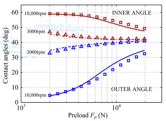
Figure 7.
The comparison of contact angles from Antoine’s model (markers) and from the present bearing model (lines).
Table 1 gives the stiffness comparison of ball bearing NSK 7014A5TYSULP4 between the NSK manual and the calculation results based on the present ball bearing model. The bearing stiffness formulas can be derived from the partial derivatives of the bearing load with respect to bearing displacement based on Equation (21). The detailed calculation process is omitted here, and a similar work can be found in [22,23,24]. It can be seen that the errors between the calculation results and manufacturer data were very small and less than 3%, which indicated that the ball bearing model was very valid.

Table 1.
The bearing stiffness comparison between the numerical calculation results and the NSK manual.
To further validate the effectiveness of the system model, a gear shaft supported by a pair of angular contact ball bearings from Tong’s work [25] was analyzed considering different shaft diameters and bearing arrangements. The bearing displacements and loads are presented in Figure 8 and Figure 9. As shown in Figure 8 and Figure 9, the results calculated by the present system model were very consistent with those from Tong’s model [25], and the difference between the results from the two different models was less than 8%, which verified the system model and the calculation procedure.
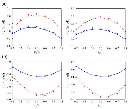
Figure 8.
The comparison of the bearing angular displacements.  ds = 35 mm,
  ds = 40 mm from Tong’s model and
  ds = 35 mm,
  ds = 40 mm from the present system model. (a) Face-to-Face arrangement; (b) Back-to-Back arrangement.
ds = 35 mm, ds = 40 mm from Tong’s model and ds = 35 mm, ds = 40 mm from the present system model. (a) Face-to-Face arrangement; (b) Back-to-Back arrangement.
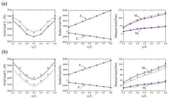
Figure 9.
The comparison of the bearing loads. ds = 35 mm, ds = 40 mm from Tong’s model and ds = 35 mm, ds = 40 mm from the present system model. (a) Face-to-Face arrangement; (b) Back-to-Back arrangement.
ds = 35 mm, ds = 40 mm from Tong’s model and ds = 35 mm, ds = 40 mm from the present system model. (a) Face-to-Face arrangement; (b) Back-to-Back arrangement.
4. Fatigue Life Model
Based on the fatigue life theory proposed by Lunberg and Palmgren [26], the basic reference rating life model of the rolling element bearing, in million revolutions, can be calculated as:
In addition:
in which the subscripts i and e refer to the inner and outer ring. The basic dynamic load rating of the inner and outer rings, , can be calculated as:
where is and the upper sign and the lower sign denote the inner- and outer-raceway contact, respectively. For the current analysis, the equivalent dynamic loads for the rotating inner ring and the fixed outer ring are calculated, respectively, as:
Based on the geometry parameters of the ball bearing, the basic dynamic load rating of the inner and outer rings can be calculated by Equation (30). The contact force distribution in each bearing is solved by the presented system model considering bearing preload and angular misalignment, then the equivalent dynamic loads of the inner and outer rings can be obtained by Equations (31) and (32). The basic reference rating life of ball bearings taking into account different preload and angular misalignment conditions is calculated according to Equations (28) and (29).
5. Results and Discussion
A sample three-bearing shaft system was investigated as shown in Figure 10, and the shaft was supported by three identical 7008C ACBBs. All ball bearings’ inner rings were perfectly fixed to the shaft. The outer ring of front bearing was free to move axially in order to apply preload, and the outer ring of each rear bearing was fixed either ideally or with a small misalignment angle caused by mounting error. The three ball bearings were assembled 32.5 mm, 187.5 mm, and 237.5 mm away from the left end of the shaft, respectively, and named as the front bearing, Rear Bearing 1 and Rear Bearing 2. The geometrical and material parameters for the bearing and shaft are given in Table 2 and Table 3, respectively. The external loads acting on the shaft (radial loads , were 1500 N and 1000 N, respectively; axial load was −1000 N; and moments , were 5000 N·mm and 6000 N·mm, respectively) were applied to the shaft node 110mm away from the left end of the shaft. The shaft rotation speed was 10,000 r/min with a centrifugal force of around 11 N for each ball element. The two axial preload methods, including constant-displacement preload and constant-force preload, were considered, and the preload was applied on the outer ring of the front bearing. The outer ring of either Rear Bearing 1 or Rear Bearing 2 was subjected to angular misalignment caused by mounting error, and only the angular misalignment around the y-axis of the bearing local coordinate system was considered here. For brevity, Case I was used to indicate that Rear Bearing 1 was subjected to angular misalignment, and Case II implied that Rear Bearing 2 was subjected to angular misalignment.
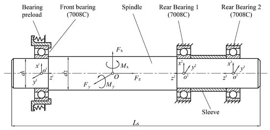
Figure 10.
Shaft-bearing system with three angular contact ball bearings.
Table 2.
The parameters of angular contact ball bearing 7008C.
Table 3.
The parameters of the shaft.
5.1. The Constant-Displacement Preload Condition
Figure 11 shows the nonlinear dependence of the basic reference rating life of all three bearing on the angular misalignment in the constant-displacement preload condition. As can be seen, the fatigue life of each bearing varied significantly with the angular misalignment, and most of them were not the highest when the angular misalignment was zero, except for that of Rear Bearing 2 in the Case II condition. For each misaligned bearing, an optimal angular misalignment existed regardless of the preload value at which the misaligned bearing had the highest fatigue life. The optimal angular misalignment values were different for the two misaligned bearings, −0.8 mrad for Rear Bearing 1 and 0 mrad for Rear Bearing 2, which mainly depended on the contact force distribution of the misaligned bearings [27]. According to SKF [28], the permissible misalignment angle was 1.2 mrad. It could be seen that the fatigue life of all bearings was very low at either 1.2 mrad or −1.2 mrad compared with that within the permissible misalignment angle, as shown in Figure 11; the angular misalignment approaching the permissible misalignment angle could lead to a significant reduction of bearing life.
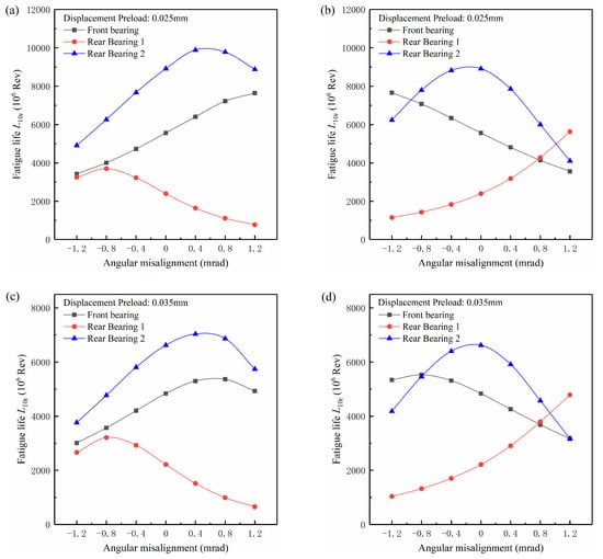
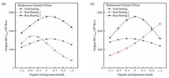
Figure 11.
The variation of bearing life with the angular misalignment in the Case I condition ((a), (c) and (e)) and the Case II condition ((b), (d) and (f)) for constant-displacement preload.
For a shaft-bearing system, the failure of any bearing will cause the system to fail. Due to the dispersion of material properties, the bearing with a high rated life may fail earlier than that with a low rated life, but the probability of this phenomenon decreases significantly as the gap between the high rated life and low rated life increases. In general, the bearing with a low rated life is more likely to fail first compared with the bearing with a high rated life. Without losing generality, it is supposed that the system life is mainly related to the bearing with the lowest rated life. The shaft fatigue life is not taken into account here. In the Case I condition, Rear Bearing 1 was misaligned. When the front bearing was preloaded by an axial displacement of 0.025 mm, the fatigue life of Rear Bearing 1 was always the lowest among the three bearings as the angular misalignment varied from −1.2 mrad to 1.2 mrad, therefore governing the system life. The shaft system had the same optimal angular misalignment, −0.8 mrad, and the same highest fatigue life with Rear Bearing 1. The highest system life was significantly greater than the system life at the angular misalignment of 0 mrad, reaching 1.55 times. As the preload displacement increased to 0.050 mm, the system life depended on the fatigue life of both Rear Bearing 1 and the preloaded front bearing, and the optimal angular misalignment turned to −0.21 mrad. The system optimal angular misalignment was no longer the same as the bearing optimal angular misalignment and approached 0 mrad, which was caused by the significant reduction of the fatigue life of the preloaded front bearing with increasing preload value. The system life at the optimal angular misalignment was only 1.12 times that at the angular misalignment of 0 mrad. The difference between the system life at the optimal angular misalignment and the system life at the angular misalignment of 0 mrad decreased with the increasing constant-displacement preload. In the Case II condition, the system life was mainly related to both the front bearing and Rear Bearing 1 due to the high fatigue life of the misaligned Rear Bearing 2. The optimal angular misalignments of the shaft system were 0.8 mrad, 0.8 mrad, and 0.21 mrad, respectively, as the preload displacement varied from 0.025 mm to 0.050 mm. The optimal angular misalignments of the shaft system for Case I and Case II were nearly opposite each other at the same preload displacement. Such a phenomenon was attributed to the negative optimal angular misalignment in the Case I condition and the positive optimal angular misalignment in the Case II condition causing a similar shaft elastic deformation, therefore producing a similar contact force distribution in Rear Bearing 1. The contact force distribution of Rear Bearing 1 at the preload displacements of 0.025 mm and 0.035 mm is given in Figure 12 to verify this point, and the contact force results at the preload displacement of 0.050 mm were omitted here.
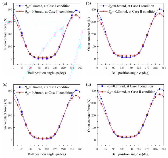
Figure 12.
The contact force distribution in Rear Bearing 1 at the optimal angular misalignment of the shaft-bearing system. The preload displacements are 0.025 mm ((a) and (b)) and 0.035 mm ((c) and (d)), respectively.
In addition, the comparison of the highest system life showed that the Case I condition could lead to a reduction of system life compared with the Case II condition, the reduction amount being from 15% to 1% with the constant-displacement preload varying from 0.025 mm to 0.050 mm. The reduction amount was significant at the low preload displacement and could be ignored at the high preload displacement.
5.2. The Constant-Force Preload Condition
Figure 13 shows the variation of bearing life with the angular misalignment in the constant-force preload condition. In order to analyze the effects of the preload method on the bearing life, the preload force was taken as 500 N, 1000 N, and 1500 N. When the shaft was running without external loads, the preload force of 500 N could cause 0.0355 mm axial displacement of the outer ring of the front bearing, which was very close to 0.035 mm, and the preload force of 1000 N could cause 0.050 mm axial displacement. Therefore, the preload force of 500 N and 1000 N at the constant-force preload could be assumed to be equivalent to the preload displacement of 0.035 mm and 0.050 mm in the constant-displacement preload, respectively. The life comparisons can be made between Figure 11c–f and Figure 13a–d. As can be seen, the two preload methods had a certain effect on the variation of the fatigue life of the preloaded front bearing with the angular misalignment. For the constant-force preload condition, the fatigue life of front bearings was basically linear with angular misalignment, and for the constant-displacement condition, a nonlinear relation could be found. The above difference was mainly due to the outer ring of the front bearing moving slightly with the angular misalignment for the constant-force preload condition, while the outer ring of the front bearing was immovable for the constant-displacement preload condition, which affected the contact force distribution in the front bearing, therefore resulting in different trends of the front bearing life with angular misalignment. With the increasing of the constant-displacement preload, the nonlinear relation between the fatigue life of the front bearing and the angular misalignment became more obvious, as shown in Figure 11. For the constant-force preload condition, the increasing preload force reduced the dependence of the front bearing life on the angular misalignment, and the relation between the front bearing life and the angular misalignment approached a horizontal line at the preload force of 1500 N, as shown in Figure 13. Among the three bearings in the shaft system, the effect of the preload method on the fatigue life of Rear Bearing 1 was the weakest, and the two preload methods only caused a small change in the fatigue life of Rear Bearing 1. From Figure 11c–f and Figure 13a–d, it can be seen that the fatigue life of Rear Bearing 1 was lowest over a wide angular misalignment range, therefore playing a significant role in the system life. Due to the effect of the preload method on the fatigue life of Rear Bearing 1 being very limited, the optimal angular misalignment and highest fatigue life for the shaft system were the same for the two preload methods.
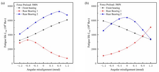
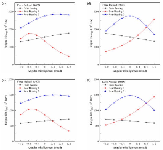
Figure 13.
The variation of the bearing life with the angular misalignment in the Case I condition ((a), (c) and (e)) and in the Case II condition ((b), (d) and (f)) for constant-force preload.
As the preload force reached 1500 N, the system life depended on the fatigue life of both the front bearing and Rear Bearing 1. The optimal angular misalignment for the shaft system was close to 0.4 mrad in the Case I condition and −0.4 mrad in the Case II condition. As mentioned above, the fatigue life of the front bearing varied slowly with angular misalignment, which resulted in very small variation of the system life near the optimal angular misalignment. Therefore, a large range, for example from −0.4 mrad to 0.4 mrad for the Case I condition and from −0.8 mrad to 0.4 mrad for the Case II condition, could be regarded as the optimal angular misalignment range of the shaft system. Such a phenomenon implied that the increasing constant-force preload could weaken the effects of angular misalignment on the system life.
6. Conclusions
In this paper, to analyze the effects on the fatigue life of bearings and the shaft system resulting from the combined preload and angular misalignment induced by inaccurate mounting, a shaft-bearing system with bearing preload and angular misalignment was investigated. By improving the computational efficiency of ball element force analysis, the system model was solved fast and reliably. Comparisons were also made to verify the correctness of the system model and calculation program. Based on the contact force distribution of ball bearings, the fatigue life of each ball bearing was obtained. The results showed that both the preload and angular misalignment had significant effects on the fatigue life of ball bearings and the shaft-bearing system.
An optimal angular misalignment existed for the shaft-bearing system and could prolong the system life. At the low preload value, the system life at the optimal angular misalignment was much higher than that at 0mrad, and such a difference decreased with the increasing preload value. The optimal angular misalignment of the shaft system was not always the same as that of the misaligned bearing, which depended on the preload value and the fatigue life of each bearing. The two preload methods, constant-displacement preload and constant-force preload, had significant effects on the variation of the preloaded bearing life with the angular misalignment, but weak effects on the highest system life. At high constant-force preload, the system life varied very slowly with angular misalignment, and an optimal angular misalignment range existed. The angular misalignment occurring on different bearings could lead to a significant difference of the highest system life when the preload value was low, but the difference could be ignored when the preload value was high.
Author Contributions
Conceptualization, Y.Z. and L.X.; Methodology, Y.Z. and M.Z.; Software, M.Z.; Validation, Y.Z. and M.Z.; Analysis, Y.Z. and Y.W.; Writing—Original Draft Preparation Y.Z., M.Z. and Y.W.; Writing—Review and Editing, Y.Z. and M.Z.; Supervision, Y.Z. and L.X. All authors have read and agreed to the published version of the manuscript.
Funding
This research received no external funding.
Acknowledgments
This work was supported by the Liaoning Provincial Natural Science Foundation of China (Grant Number 20170540739), the Open Fund of Key Laboratory of Vibration and Control of Aero-Propulsion System Ministry of Education, Northeastern University (Grant Number VCAME201802), and the Natural Science Foundation of China (Grant Number U1708255).
Conflicts of Interest
The authors declared no potential conflict of interest with respect to the publication of this article.
Nomenclature
| major semi-axis for ball-raceway contact ellipse, mm | |
| minor semi-axis for ball-raceway contact ellipse, mm | |
| ball diameter, mm | |
| bearing pitch diameter, mm | |
| inner diameter of bearing, mm | |
| outer diameter of bearing, mm | |
| thickness of bearing, mm | |
| groove curvature coefficients of outer raceway | |
| groove curvature coefficients of inner raceway | |
| mass moment of inertia, kg·mm2 | |
| density, kg/m3 | |
| ball mass, kg | |
| number of beam elements | |
| number of balls | |
| initial contact angle, rad | |
| contact angle at ball-outer raceway contact, rad | |
| contact angle at ball-inner raceway contact, rad | |
| ball pitch angle, rad | |
| angular speed of inner ring/shaft around the bearing axis, rad/s | |
| ball orbital speed around the bearing axis, rad/s | |
| ball spinning speed around its own axis, rad/s | |
| friction moment at ball-outer raceway contact due to spinning, N·mm | |
| friction moment at ball-inner raceway contact due to spinning, N·mm | |
| second kind of elliptic integral function | |
| contact force at ball-inner raceway contact, N | |
| contact force at ball-outer raceway contact, N | |
| ball centrifugal force, N | |
| gyroscopic moment, N·mm | |
| friction force at ball-inner raceway contact, N | |
| friction force at ball-outer raceway contact, N | |
| bearing force applied on the inner ring of ball bearing along x-axis of bearing local coordinate system, N | |
| bearing force applied on the inner ring of ball bearing along y-axis of bearing local coordinate system, N | |
| bearing force applied on the inner ring of ball bearing along z-axis of bearing local coordinate system, N | |
| moment applied on the inner ring of ball bearing around x-axis of bearing local coordinate system, N·mm | |
| moment applied on the inner ring of ball bearing around y-axis of bearing local coordinate system, N·mm | |
| external load vector applied on the shaft nodes, N | |
| ball-raceway friction coefficient | |
| initial position of ball center | |
| final position of ball center | |
| outer raceway groove curvature center | |
| initial position of inner raceway groove curvature center | |
| final position of inner raceway groove curvature center | |
| axial distance between ball center and outer raceway groove curvature center , mm | |
| radial distance between ball center and outer raceway groove curvature center , mm | |
| translational displacement of inner ring along x-axis of bearing local coordinate system, mm | |
| translational displacement of inner ring along y-axis of bearing local coordinate system, mm | |
| translational displacement of inner ring along z-axis of bearing local coordinate system, mm | |
| angular displacement of inner ring around x-axis of bearing local coordinate system, rad | |
| angular displacement of inner ring around y-axis of bearing local coordinate system, rad | |
| ball-outer raceway contact deformation, mm | |
| ball-inner raceway contact deformation, mm | |
| rotational speed of inner ring/shaft, rpm | |
| radius of locus of inner raceway groove curvature centers, mm | |
| ball azimuth angle, rad | |
| Poisson’s ratio | |
| deflection coefficient at ball and outer raceway contact, N/mm1.5 | |
| deflection coefficient at ball and inner raceway contact, N/mm1.5 | |
| groove curvature radius of inner raceway, mm | |
| global stiffness matrix of the shaft | |
| stiffness matrix of the beam element | |
| displacement vector of the shaft nodes, mm | |
| modulus of elasticity, GPa | |
| moment of inertia of the shaft section, mm4 | |
| length of beam element, mm | |
| total length of the shaft, mm | |
| number of angular contact ball bearings supporting the shaft | |
| calculation error of ball spinning speed | |
| calculation error of ball orbit speed | |
| calculation error of ball pitch angle | |
| axial displacement caused by constant-displacement preload or constant-force preload, mm | |
| angular misalignment of outer ring of ball bearing around x-axis of bearing local coordinate system, mrad | |
| angular misalignment of outer ring of ball bearing around y-axis of bearing local coordinate system, mrad | |
| basic reference rating life of bearing, in million revolutions | |
| basic reference rating life of inner ring, in million revolutions | |
| basic reference rating life of outer ring, in million revolutions | |
| basic dynamic load rating of inner ring, N | |
| basic dynamic load rating of outer ring, N | |
| equivalent dynamic load for rotating inner ring, N | |
| equivalent dynamic load for fixed outer ring, N |
References
- Jin, Y.; Yang, R.; Lei, H.; Chen, Y.; Zhang, Z. Experiments and Numerical Results for Varying Compliance Contact Resonance in a Rigid Rotor–Ball Bearing System. J. Tribol. 2017, 139, 041103. [Google Scholar] [CrossRef]
- Yang, Y.; Yang, W.; Jiang, D. Simulation and experimental analysis of rolling element bearing fault in rotor-bearing-casing system. Eng. Fail. Anal. 2018, 92, 205–221. [Google Scholar] [CrossRef]
- Wang, H.; Han, Q.; Zhou, D. Nonlinear dynamic modeling of rotor system supported by angular contact ball bearings. Mech. Syst. Signal Process. 2017, 85, 16–40. [Google Scholar] [CrossRef]
- Cao, H.; Niu, L.; Xi, S.; Chen, X. Mechanical model development of rolling bearing-rotor systems: A review. Mech. Syst. Signal Process. 2018, 102, 37–58. [Google Scholar] [CrossRef]
- Harris, T.A. The Effect of Misalignment on the Fatigue Life of Cylindrical Roller Bearings Having Crowned Rolling Members. J. Tribol. 1969, 91, 294–300. [Google Scholar] [CrossRef]
- Hagiu, G.; Gafitanu, M. Preload-service life correlation for ball bearings on machine tool main spindles. Wear 1994, 172, 79–83. [Google Scholar] [CrossRef]
- Hwang, Y.-K.; Lee, C.M. A review on the preload technology of the rolling bearing for the spindle of machine tools. Int. J. Precis. Eng. Manuf. 2010, 11, 491–498. [Google Scholar] [CrossRef]
- Tong, V.-C.; Hong, S.-W. Fatigue life of tapered roller bearing subject to angular misalignment. Proc. Inst. Mech. Eng. Part C J. Mech. Eng. Sci. 2015, 230, 147–158. [Google Scholar] [CrossRef]
- Yang, L.; Xu, T.; Xu, H.; Wu, Y. Mechanical behavior of double-row tapered roller bearing under combined external loads and angular misalignment. Int. J. Mech. Sci. 2018, 142, 561–574. [Google Scholar] [CrossRef]
- Warda, B.; Chudzik, A. Fatigue life prediction of the radial roller bearing with the correction of roller generators. Int. J. Mech. Sci. 2014, 89, 299–310. [Google Scholar] [CrossRef]
- Warda, B.; Chudzik, A. Effect of ring misalignment on the fatigue life of the radial cylindrical roller bearing. Int. J. Mech. Sci. 2016, 111, 1–11. [Google Scholar] [CrossRef]
- Jiang, S.; Mao, H. Investigation of variable optimum preload for a machine tool spindle. Int. J. Mach. Tools Manuf. 2010, 50, 19–28. [Google Scholar] [CrossRef]
- Xu, T.; Xu, G.; Zhang, Q.; Hua, C.; Tan, H.; Zhang, S.; Luo, A. A preload analytical method for ball bearings utilising bearing skidding criterion. Tribol. Int. 2013, 67, 44–50. [Google Scholar] [CrossRef]
- Than, V.-T.; Huang, J.H. Nonlinear thermal effects on high-speed spindle bearings subjected to preload. Tribol. Int. 2015, 96, 361–372. [Google Scholar] [CrossRef]
- Zhang, J.; Fang, B.; Hong, J.; Zhu, Y. Effect of preload on ball-raceway contact state and fatigue life of angular contact ball bearing. Tribol. Int. 2017, 114, 363–372. [Google Scholar] [CrossRef]
- Ding, C. Raceway control assumption and the determination of rolling element attitude angle. Chin. J. Mech. Eng. 2001, 37, 58–61. (In Chinese) [Google Scholar] [CrossRef]
- Harris, T.A.; Kotzalas, M.N. Rolling Bearing Analysis; Taylor & Francis: Boca Raton, FL, USA, 2007. [Google Scholar]
- Logan, D.L. A First Course in the Finite Element Method; Cengage: Boston, MA, USA, 2012. [Google Scholar]
- Glover, F. A Template for Scatter Search and Path Relinking, Lecture Notes in Computer Science 1363; Springer: Berlin/Heidelberg, Germany, 1998. [Google Scholar]
- Ugray, Z.; Lasdon, L.; Plummer, J.; Glover, F.; Kelly, J.; Martí, R. Scatter Search and Local NLP Solvers: A Multistart Framework for Global Optimization. INFORMS J. Comput. 2007, 19, 328–340. [Google Scholar] [CrossRef]
- Antoine, J.-F.; Abba, G.; Molinari, A. A New Proposal for Explicit Angle Calculation in Angular Contact Ball Bearing. J. Mech. Des. 2006, 128, 468–478. [Google Scholar] [CrossRef]
- Zhang, X.; Han, Q.; Peng, Z.-K.; Chu, F. Stability analysis of a rotor–bearing system with time-varying bearing stiffness due to finite number of balls and unbalanced force. J. Sound Vib. 2013, 332, 6768–6784. [Google Scholar] [CrossRef]
- Yang, Z.; Chen, H.; Yu, T. Effects of rolling bearing configuration on stiffness of machine tool spindle. Proc. Inst. Mech. Eng. Part C J. Mech. Eng. Sci. 2017, 232, 775–785. [Google Scholar] [CrossRef]
- Zhang, J.; Fang, B.; Zhu, Y.; Hong, J. A comparative study and stiffness analysis of angular contact ball bearings under different preload mechanisms. Mech. Mach. Theory 2017, 115, 1–17. [Google Scholar] [CrossRef]
- Tong, V.-C.; Hong, S.-W. Study on the running torque of angular contact ball bearings subjected to angular misalignment. Proc. Inst. Mech. Eng. Part J J. Eng. Tribol. 2017, 232, 890–909. [Google Scholar] [CrossRef]
- Lundberg, G.; Palmgren, A. Dynamic capacity of rolling bearings. In Acta Polytechnica, Mechanical Engineering Series I; Royal Swedish Academy of Engineering Sciences: Stockholm, Sweden, 1947; pp. 1–50. [Google Scholar]
- Li, X.; Li, H.; Hong, J.; Zhang, Y. Heat analysis of ball bearing under nonuniform preload based on five degrees of freedom quasi-static model. Proc. Inst. Mech. Eng. Part J J. Eng. Tribol. 2015, 230, 709–728. [Google Scholar] [CrossRef]
- SKF Group. SKF General Catalogue 6000/I EN; SKF Group: Gothenburg, Sweden, 2008. [Google Scholar]
© 2020 by the authors. Licensee MDPI, Basel, Switzerland. This article is an open access article distributed under the terms and conditions of the Creative Commons Attribution (CC BY) license (http://creativecommons.org/licenses/by/4.0/).