A Novel Method for Tool Identification and Wear Condition Assessment Based on Multi-Sensor Data

Abstract

The development of industry 4.0 has put forward higher requirements for modern milling technology. Monitoring the degree of milling tool wear during machine tool processing can improve product quality and reduce production losses. In the machining process of machine tools, many kinds of tools are usually used, and the signal characteristics of various sensors of different tools are different. Therefore, before the tool wear assessment, this paper identified the tool type according to the spindle current data. After the tool type recognition, this paper evaluates the tool wear degree according to the tool force data, vibration data, acoustic emission signal, and other multi-sensor data. Firstly, the Elman neural network and Adaboost algorithm are combined to construct the Elman_Adaboost strong predictor. Then, the variance and mean of seven sensor data were selected as the characteristic quantities to input the strong predictor. Finally, three wear quantities were obtained to measure the wear degree of the tool. The method proposed in this paper is implemented by Matlab, and the validity of this method is verified using the competition data provided by PHM (Prognostics and Health Management) Society. The results show that the average evaluation accuracy of the same tool wear is more than 92%, and that of the similar tool wear is more than 85%.

1. Introduction

HSC (high speed cutting) is one of the representatives of advanced manufacturing technology, which has the advantages of high precision, high speed, and high quality [1,2]. In the milling process, the milling cutter directly contacts the workpiece, and the tool wear will directly cause the surface quality and machining accuracy of the workpiece to decline. Tool breakage will cause chatter, tool breakage and other phenomena, and even cause machine tool damage and production accidents [3,4]. In order to improve the wear resistance of cutting tools, a lot of research has been undertaken [5,6]. According to the statistical research, when the automatic production equipment is equipped with a tool state detection system, the downtime will be reduced by 75%, the utilization rate of machine tools will be increased by at least 50%, and the total production efficiency will be increased by 10%–60% [7]. Therefore, the real-time monitoring of tool wear is of great significance to improve product quality and reduce processing costs [8,9,10].

At present, many achievements have been made in the research of tool wear evaluation. In view of the massive data processing problem under the background of industry 4.0, [11] uses CNN (Convolutional Neural Networks) neural network algorithm to predict and classify the tool wear degree according to the collected cutting force, and proposes a relatively complete processing system—however, the overall evaluation accuracy is low. In the research on tool signal processing. Yongjiao Chi combined tool wear with monitoring signal analysis based on modal analysis, and proposed a new tool wear estimation method, which used ensemble empirical mode decomposition (EEMD) to extract the signal characteristics of the processing process for real-time tool wear assessment [12]. Soham Mehta put forward a method of measuring tool wear directly by using a visual system. This method uses Matrox software to process the gray image obtained by charge coupled device camera and to acquire the tool wear degree [13]. Driven by the monitored big data, Kunpeng Zhu systematically investigates the key issues for tool condition monitoring, such as machining dynamics, intelligent tool wear monitoring and compensation algorithms, heterogeneous big data fusion, and deep learning methods. Under this scheme, it develops the smart tool condition monitoring system that could improve the computer numerical control machining precision and productivity significantly [14]. In the optimization of tool wear condition monitoring system, Xincheng Cao combined derived wavelet frames (DWFs) and CNN. By decomposing the original signal into different bandwidth, different center frequency bands, the reconstructed sub signal is superposed into two-dimensional signal matrix, which matches the structure of two-dimensional CNN, and then the two-dimensional signal matrix is identified by neural network [15]. Zhou Haibo obtained the approximate linear relationship between the logarithm of cutting speed and the logarithm of milling distance based on the experiment of high-speed milling titanium alloy TC4 with cemented carbide tools and constructed the prediction model of tool wear [16]. However, the prediction of tool wear caused by cutting speed is only realized, and the prediction accuracy is too low. In the multi-disciplinary research of multi-sensor fusion technology, due to its versatility and wide application fields, it has attracted more and more interest, and it is also a worthy direction in the research of tool wear [17]. Therefore, in order to solve the problem of tool wear evaluation, this paper proposes a tool wear prediction model based on the multi-sensor Elman_Adaboost strong predictor. Currently AdaBoost is mainly used for classification [18,19,20]. In this paper, the function of AdaBoost is extended to predict. Elman neural network is used as a weak predictor to train Elman neural network to form a strong predictor, and an algorithm of tool wear prediction based on Elman_AdaBoost strong predictor is established to make the system have Elman’s adaptability to time-varying characteristics. In order to verify the effectiveness of the algorithm, this paper uses the data provided by the PHM society in the data competition held in 2010 to test and verify the algorithm.

In addition, the process of machine tool processing usually needs to use a variety of tools, so the process of tool replacement, the cutting force of different tools, vibration signals, acoustic emission signals, and other sensor signals are different. Therefore, before evaluating tool wear, it is necessary to identify the type of tool currently in use. Aiming at the problem of tool type identification, this paper presents a tool identification method based on spindle current.

The rest of this paper is organized as follows. In Section 2, the framework and algorithm of tool wear prediction system are introduced. The tool recognition scheme based on spindle current proposed in this paper is described in Section 3. In Section 4, the tool wear prediction based on Elman_AdaBoost model is introduced and the results are analyzed. Finally, Section 5 is the summary of the paper.

2. System Framework and Platform Construction

2.1. System Framework

The framework of tool wear evaluation system based on spindle current and multi-sensor data is shown in Figure 1. Firstly, this method analyzes the working state of the machine tool through the spindle current, and determines the current tool type, so as to prepare for the subsequent prediction of tool wear state. Secondly, the separation tool is used to properly process the collected signals and extract the mean value, variance, and other characteristics of the signals. Finally, according to the extracted feature information, the wear degree is predicted by the neural network method.

2.2. Platform Construction

Tool state detection methods are divided into direct and indirect methods. The direct method can identify the blade appearance, surface quality or geometric shape changes, and it can generally only be carried out when not cutting. It has two obvious disadvantages: first, is the requirement of shutdown detection and occupied production hours; secondly, it is impossible to detect the tool in the process of sudden damage, so that its application is limited. The indirect measurement method is to use the effect of the state of tool wear or about to be damaged on different working parameters to measure the parameters reflecting the degree of various effects of tool wear and damage, which can be detected during cutting without affecting the cutting process [21]. Therefore, referring to the wear data of milling cutters from PHM society, this paper proposes to use an indirect method to build a multi-sensor platform by collecting three-axis force data, three-axis vibration data, and acoustic emission signals.

Since the tool must be detected quickly and the acquisition frequency of the sensor is required to be high, the sensor adopts three-axis force sensor 1303M-160, three-axis vibration sensor CT100SLC and acoustic emission sensor ae144sa40-BNC. These three sensors are used to collect the force, vibration frequency, and acoustic emission signal of the tool, which are respectively installed on the workbench and spindle of the machining center. All the signals sent by the sensors are amplified and filtered, then fed back through the rate adjustment, and finally entered into the computer for data acquisition. In addition, the acoustic emission signals of tool breakage are mostly in the frequency range 80–400 KHZ, and the signal acquisition frequency range of AE sensor AE144SA40-BNC is 50 to 500 KHZ. Since the data acquisition speed of the general upper computer is slow, in order to meet the higher sampling frequency, this paper uses NI-PCI-MIO-16E-1 data acquisition card with the maximum sampling rate of 1.25 MHZ to send data. The signal from the motor current sensor of the spindle can be input into the computer without further processing.

3. Tool Identification

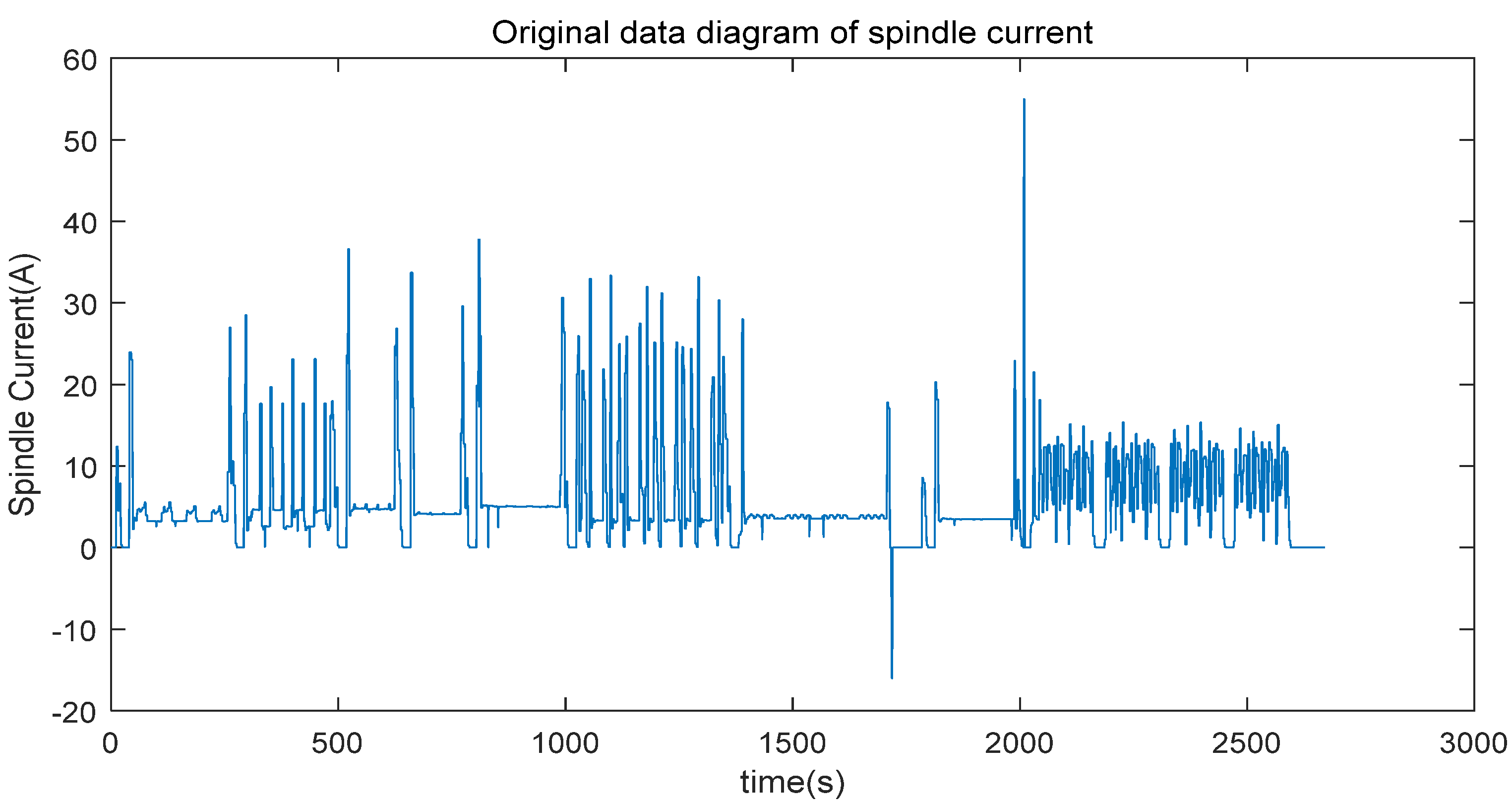
In the process of machine tool processing, we need to use a variety of tools, as there is a process of tool replacement. The cutting force, vibration signal, and acoustic emission signal of different cutting tools are different. Therefore, it is necessary to identify the types of tools currently used in order to further predict the wear of current tools. When processing the machine tool, the tool processing sequence is known, and the current tool can be accurately identified by detecting the spindle current. When the spindle current is 0 and maintained for a period of time, it means that the machine tool stops working, and the tool is changed during this period. In the actual machining process, the spindle current data is affected by the starting current and the braking current, and the fluctuation is relatively large. Therefore, it is necessary to preprocess the spindle current data. This paper takes the spindle current data of a process (nine knives in total) as an example, and the original data is shown in Figure 2, where the horizontal axis is the sampling time, and the vertical axis is the spindle current.

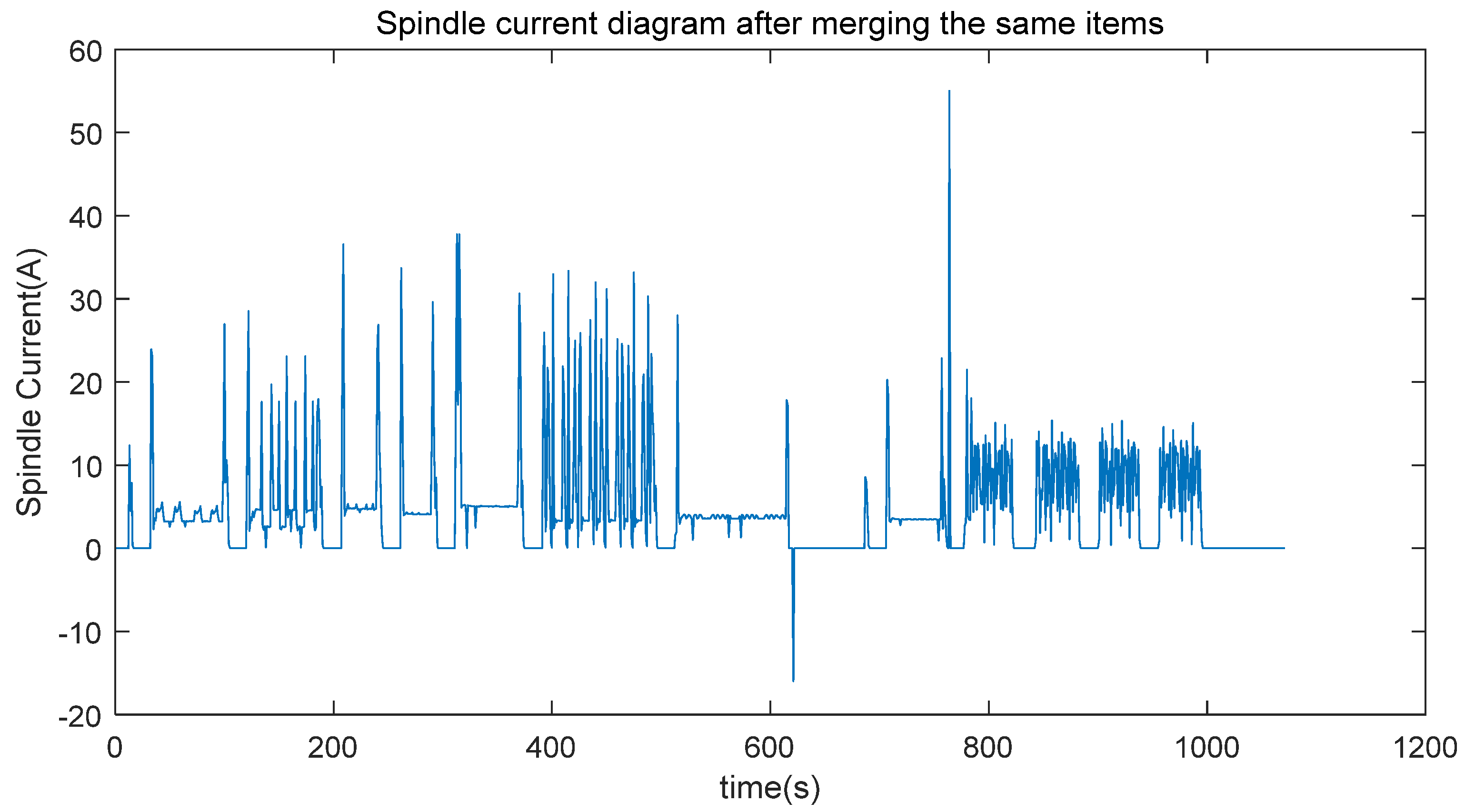
The amount of original data is large, and the adjacent data is mostly repetitive data, so the amount of data can be reduced by removing the adjacent same data while retaining the original data characteristics, so as to reduce the computational complexity. The spindle current data with the adjacent same current data removed is shown in Figure 3.

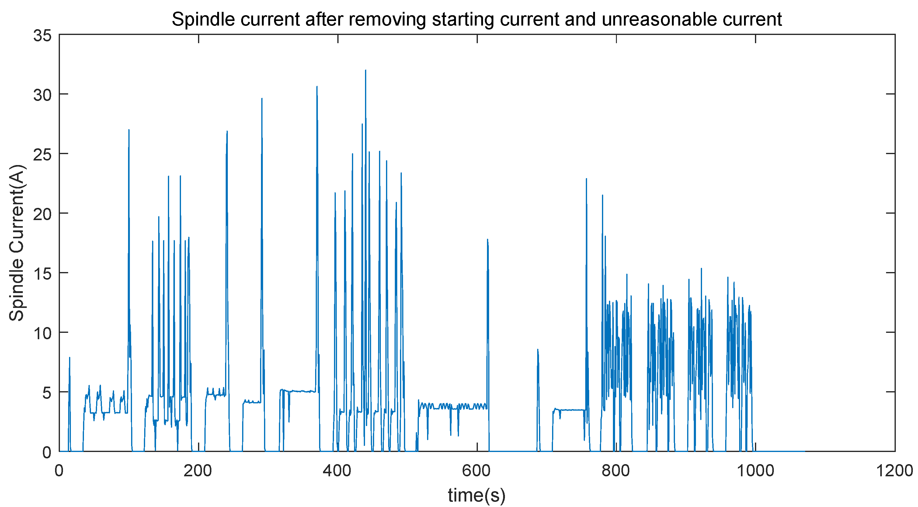
As can be seen from Figure 3, the processed current data volume is about half of the original data volume, but its waveform is basically consistent with Figure 2. When the spindle starts to rotate, there will be a large starting current, which will affect the tool recognition. The starting current can be filtered by detecting whether the machine tool is currently in a tool change state and then setting the current threshold. It can be seen from the original data that there are two maximum jumping points in the current value, which can be filtered by setting the current threshold. Finally, the data after filtering the starting current and the jump current of the main shaft can be obtained as shown in Figure 4.

It can be seen from Figure 3 that when the current value is 0, the spindle is in a stalled state, but there will be some jumping noise current during the spindle stalled process. It is known that nine kinds of tools are used in this process. In this paper, the use time of each tool is set as the threshold value to filter the fluctuation current when the tool stops running, and then judge and eliminate the spindle brake current by judging whether the spindle stops running. The data is as shown in Figure 5.

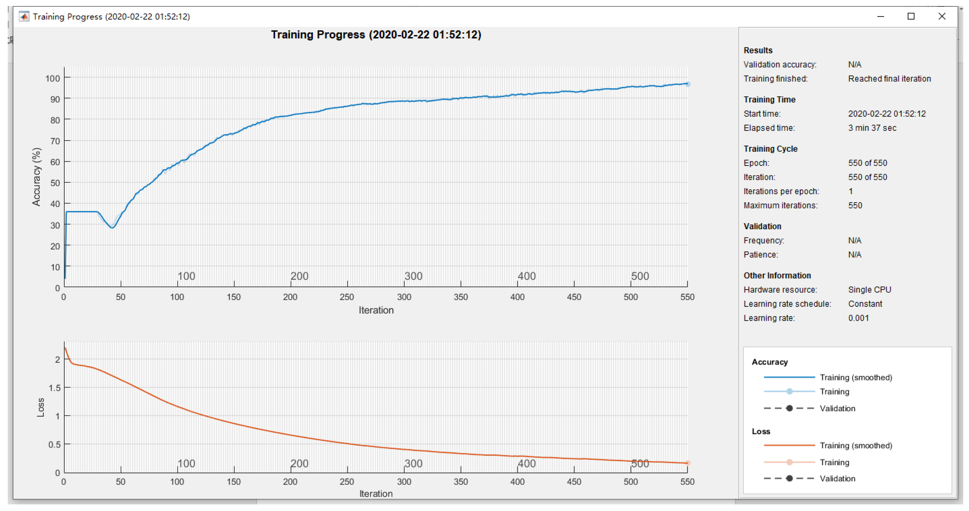
It can be seen from Figure 5 that the spindle current data of the tool changes obviously with the working time of the tool and has obvious characteristics in the time domain. Therefore, this paper adopts LSTM (Long Short-Term Memory) algorithm to build a tool recognition model and takes the processed current data as the input of the system to train the system. When the tool is to be identified, it is only necessary to use the current spindle current signal as the system input, and the output is the tool sequence of the tool currently being processed. Since this paper uses a basic LSTM neural network, it will not be discussed here. Figure 6 shows the training process of LSTM tool recognition network.

4. Tool Wear Assessment

4.1. Elman and Adaboost

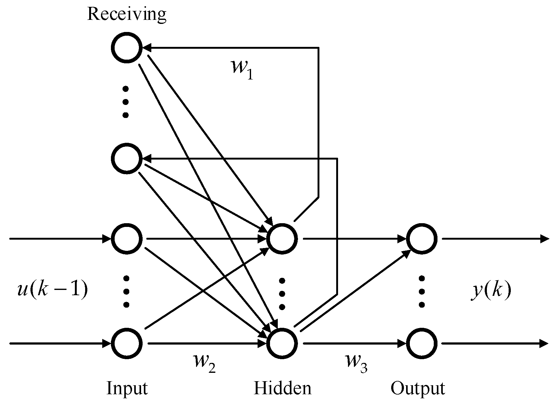
Elman neural network is a typical dynamic recurrent neural network [22]. As shown in Figure 7, on the basis of the BP neural network, a support layer is added on the hidden layer. The receiving layer has output delay and storage for the hidden layer. The role, and the receiving layer then applies the output to the input of the hidden layer, making it sensitive to historical data, increasing the network’s ability to process dynamic information.

The Elman network nonlinear state space expression is:

$$y(k)=g(w_3·x(k)),$$

(1)

$$x(k)=f(w_1·x_c(k)+w_2·(u(k-1))),$$

(2)

$$x_c(k)=x(k-1),$$

(3)

where $y$ is the $m$-dimensional output node vector;$x$ is the $n$-dimensional intermediate layer node unit vector; $u$ is the $r$-dimensional input vector; $x_c$ is the $n$-dimensional feedback state vector; $w^3$ is the connection weight from the middle layer to the input layer; $w^2$ is the connection weight from the input layer to the middle layer; $w^1$ is the connection weight from the receiving layer to the middle layer; $g(*)$ is the transfer function of the output neuron, which is a linear combination of the output of the middle layer; $f(*)$ is the transfer function of the middle layer neurons, and the $S$ function is often used.

Adaboost is an iterative algorithm whose idea is to combine the outputs of several “weak” classifiers to produce an effective classification [23]. The main steps are as follows: firstly, the weak learning algorithm and the sample space $(x,y)$ are given, and the training data of group $m$ are found from the sample space. The weight of each group of training data is $1/m$. Then, the weak learning algorithm is used to perform iterative operation $T$ times. After each operation, the weight distribution of the training data is updated according to the classification results. For the training individuals who fail in classification, a large weight is given, and the training individuals are paid more attention to in the next iteration operation.

The algorithm steps are as follows:

(1)

Data selection and network initialization. Select a group of training data randomly from the sample space, initialize the distribution weight $D_t(i)=1/m$ of the test data, determine the neural network structure according to the dimension of sample input and output, and initialize the BP neural network weight and threshold.

(2)

Weak classifier prediction. When the t th weak classifier is trained, the BP neural network is trained with the training data and the training data output is predicted to obtain the prediction error $e_t$ of the prediction sequence $g(t)$. The calculation formula of $e_t$ is as follows:

$$e_t={\displaystyle \sum _i{D}_i(i)},i=1,2,\cdots m(g(t)\ne y),$$

(4)

where $g(t)$ is the prediction classification result and $y$ is the expected classification result.

(3)

Calculate the weight of the predicted sequence. According to the prediction error $e_t$ of the prediction sequence $g(t)$, the weight $a_t$ of the sequence is calculated. The calculation formula of $a_t$ is as follows:

$$a_t=\frac{1}{2}\ln [(1-e_t)/e_t].$$

(5)

(4)

Weight adjustment of test data. Adjust the weight of the next round of training samples according to the prediction sequence weight $a_t$, and the adjustment formula is:

$$D_{t+1}(i)=\frac{D_t(i)}{B_t}\ast \exp [-a_t·y_i·g_t(x_i)],i=1,2,\cdots m,$$

(6)

where $B_t$ is the normalization factor. The purpose is to make the sum of distribution weights equal to 1 when the weight proportion is constant.

(5)

Construct strong prediction function. After training $T$ round, the weak prediction function $f(g_t,a_t)$ of $T$ group is obtained, and the strong classification function $h(x)$ is obtained by combining the weak prediction function $f(g_t,a_t)$ of $T$ group.

$$h(x)=sign[{\displaystyle \sum _{t=1}^T{a}_t·}f(g_t,a_t)],t=1,2,\cdots T.$$

(7)

4.2. Feature Selection

This paper uses Elman algorithm for each weak classifier in Adaboost and combines Adaboost and Elman algorithms to make it more adaptive. In order to verify the effectiveness of the algorithm, this paper uses the data provided by PHM Society in the data competition held in 2010.

The data included 315 cases (progressive wear) for three categories of cutters. The seven data collected are: X-axis force data, Y-axis force data, z-axis force data, X-axis vibration data, Y-axis vibration data, z-axis vibration data, AE-RMS (Root of Mean Square of Acoustic Emission), the data acquisition frequency is up to 50 khz, and the data of various wear conditions are comprehensive and rich, with high authenticity. Take the X-axis force data, X-axis vibration data, and AE-RMS of tool 1 as examples, compare the wear degree 1 with the wear degree 315, and the results are shown in Figure 8:

It can be seen from Figure 8 that the “amplitude” and “degree of oscillation” of the data collected by the sensor increase significantly with the deepening of tool wear. Therefore, this paper uses the mean and variance of the data collected by the sensor in a time as the data characteristics. The variation curve of variance and mean value of seven sensor data with the degree of tool wear is shown in Figure 9, where the x-axis indicates that the wear degree of the tool is gradually deepened from 1 to 315—which is abstract data—so there is no unit and the y-axis indicates the value after normalizing the variance and average value to the [−1,1] interval.

It can be seen from Figure 9 that with the deepening of tool wear, the data of mean value and variance value are basically in an increasing state, and the variance is more obvious. PHM also provides three wear quantities (flute1, flute2, flute3) to characterize the wear degree. Figure 10 shows the change curve of tool 1 wear with wear degree—hereinafter referred to as wear curve.

Based on the wear curves of the three tools, this paper sets the range of tool wear in three stages to determine the current wear status of the tools as shown in

Table 1. Three tool wear thresholds.

Cutting Tool	Early	Middle	Late
First	Flute1 < 87	Flute1∈(87,110)	Flute1 > 110
	and	or	and
	Flute2 < 93	Flute2∈(93,110)	Flute2 > 110
	and	or	and
	Flute3 < 93	Flute3∈(93,120)	Flute3 > 120
Second	Flute1 < 65	Flute1∈(65,105)	Flute1 > 105
	and	or	and
	Flute2 < 65	Flute2∈(65,105)	Flute2 > 105
	and	or	and
	Flute3 < 65	Flute3∈(65,105)	Flute3 > 105
Third	Flute1 < 87	Flute1∈(87,134)	Flute1 > 134
	and	or	and
	Flute2 < 97	Flute2∈(97,134)	Flute2 > 134
	and	or	and
	Flute3 < 83	Flute3∈(83,139)	Flute3 > 139

.

4.3. Algorithm Implementation

In this paper, the wear of the tool is evaluated by building an Elman-Adanoost neural network system. The mean value and variance of the original tool sensor data were input into the neural network as characteristic signals. The training output results were set by setting the threshold value, that is, the three states corresponding to the wear degree: the early wear state: [1,0], the middle wear state: [0,1,0], and the late wear state: [0,0,1]. The evaluation result classification procedure is shown as follows:

(1)

Set thresholds to classify evaluation results, the specific algorithm is shown in Algorithm 1.

Algorithm 1 Classification algorithm

Input: Characteristics of the variable, input_train

Output: Wear cycle, output_train

input_train = data_1(:,1:14);

output1_train = data_1 (:,15:17);

for i = 1:315

if output1_train (i,1) < 87 && output1_train (i,2) < 93 && output1_train (i,3) < 93

output_train(i,:) = [1,0,0];

elseif output1_train (i,1) > 110 && output1_train (i,2) > 110 && output1_train (i,3) > 120

output_train(i,:) = [0,0,1];

else

output_train(i,:) = [0,1,0];

end

end

(2)

Construct and train the neural network and normalize the input data, the specific algorithm is shown in Algorithm 2.

Algorithm 2 Training algorithm

Input: Characteristics of the variable, input_train

for i=1:K

[inputn,inputps]=mapminmax(input_train);

threshold=[−1,1; −1,1; −1,1; −1,1; −1,1; −1,1; −1,1; −1,1; −1,1; −1,1; −1,1; −1,1; −1,1; −1,1;]

net=newelm(threshold,[20,3],{‘tansig’,’purelin’});

net.trainparam.epochs=500;

net. trainparam.show=20;

net. trainparam.goal=0.0001;

net=init(net);

net=tarin(net,inputn,output_train);

test_simu1=sim(net,inputn);

inputn_test=mapminmax(‘apply’,input_test,inputps);

test_simu(1,i)={sim(net,input_test)};

(3)

Adaboost algorithm code implementation (at value adjustment, D value adjustment), the specific algorithm is shown in Algorithm 3.

Algorithm 3 Adaboost algorithm

Input: Characteristics of the variable, input_train

for j=1:nn

kk1(j)=find(test_simu1(:,j) == max(test_simu1(:,j)));

kk2(j)=find(output_train(:,j) == max(output_train (:,j)));

if kk1(j) ~= kk2(j)

Error(i)= Error(i)+D(i,j);

count_num(i)= Count_num(i)+1;

gy(j) = −1 * max(test_simu1(:,j))/sum(test_simu1(:,j));

else

gy(j) = 1 * max(test_simu1(:,j))/sum(test_simu1(:,j));

end

end

if error(i) ~= 0

at(i) = 0.5*log((1-error(i))/error(i));

else

at(i)=3;

end

for j=1:nn

D(i+1,j)=D(i,j)*exp(-at(i)*gy(j));

end

Dsum=sum(D(i+1,:));

D(i+1,:)=D(i+1,:)/Dsum;

After the forecast is completed, we can make a reasonable assessment of the result. If the predicted result differs too much from the previously predicted amount of wear, we collect the signal again and then predict the degree of wear again. If the error is still too large, we judge whether the cutter has broken or the device to be processed is wrong and give an alarm to remind the construction personnel. If the difference between this result and the previously predicted wear conforms to the wear curve, the current result is reasonable.

After the training is completed, the tool wear degree evaluation system has been successfully constructed. After collecting various types of data for feature processing, it is used as the input of the system, and the output is the predicted degree of tool wear, which is the estimated tool state.

4.4. Result Analysis

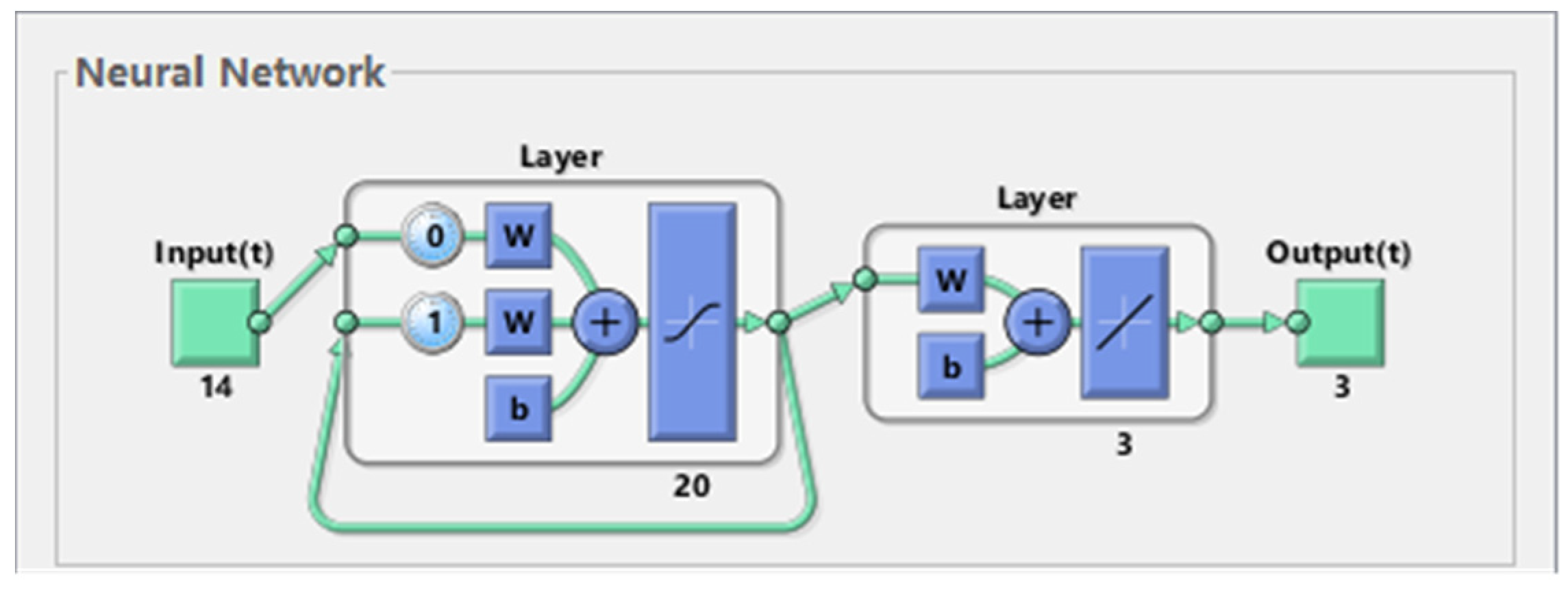
The related principles of Elman_AdaBoost have been introduced. Combined with the above data analysis, each knife contains 315 sets of data, each set of data contains 14 inputs and 3 outputs. In this paper, according to the ratio of 7:3, 215 sets of data were randomly selected as training data and 100 sets of data were used as test data to test the Elman_AdaBoost model. In combination with AdaBoost algorithm, 10 Elman weak classifiers are set up. Each Elman weak classifier is an Elman neural network. The network design structure is as follows:

(1)

Input layer design: In pattern recognition, the number of input layer nodes is equal to the number of features of training samples; that is, 14 feature values of input samples are taken as the input of the network, and the number of input nodes is 14.

(2)

Output layer design: The output node is the three wear states of the tool, that is, the output node is 3.

(3)

Hidden layer design: The number of hidden layer nodes is calculated preliminarily according to $k=\sqrt{a+b}+c,c\in [1,10]$ and then the final number of hidden layer nodes is determined by repeated experiments. After repeated experiments, the number of hidden layers is determined to be 20.

(4)

Bearing layer design: According to the principle of Elman neural network, the number of receiving layers should be equal to the number of hidden layers, so the receiving layer is 20.

The final Elman network model structure is shown in Figure 11, which is a ‘7-20-20-3’ structure. This paper sets the maximum number of iterations to 500 with an expected error of 0.0001.

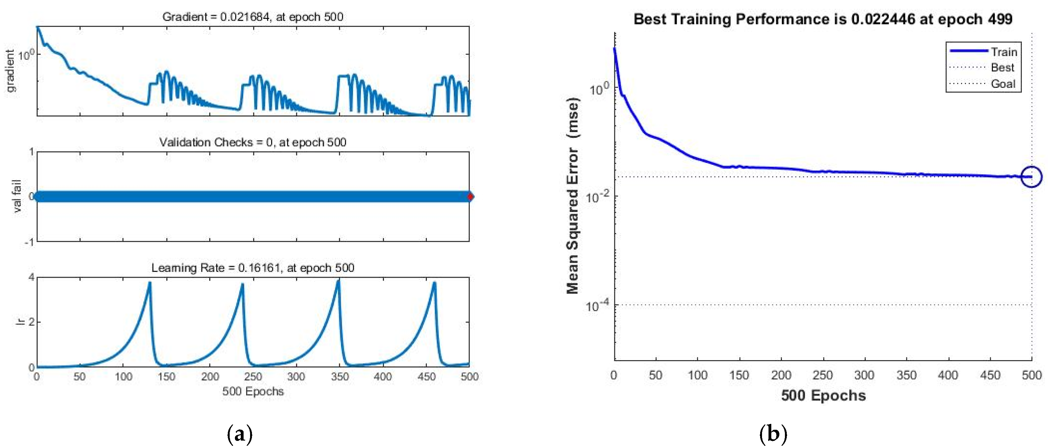
Taking an Elman network as an example, the training process information is shown in Figure 12a, which shows the gradient value, generalization ability and learning rate of the neural network changing with the number of iterations, and the training target error is shown in Figure 12b.

This paper uses the first knife as an example to test the nonlinear fitting and classification performance of the Elman_Adaboost model. according to the ratio of 7:3, 215 sets of data were randomly selected as training data and 100 sets of data were used as test data. We get three inputs for any set of inputs, and compare them with the actual output. The error results are shown in Figure 13.

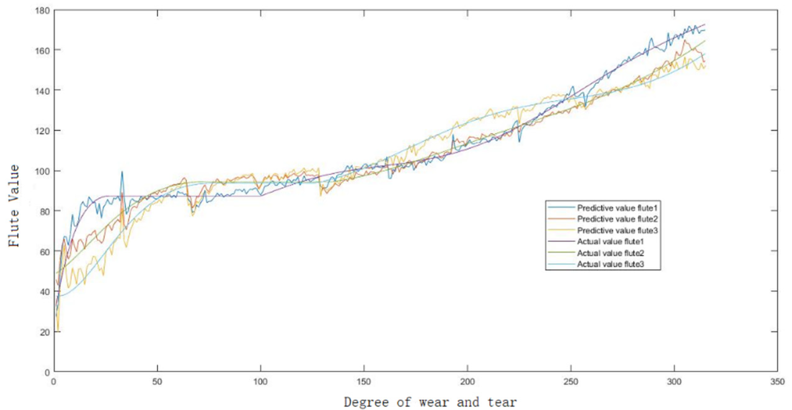
Based on this model, 100 groups of prediction data of three knives were classified into wear period. The results obtained are shown in

Table 2. Wear accuracy prediction results of three tools.

Cutting Tool	Early	Middle	Late
First	0.8333	0.9623	0.9512
Second	0.8643	0.9697	0.9241
Third	0.9529	0.9773	0.9526

and Figure 14.

According to the results, the classification accuracy of this model is still high. Considering the commonness of tool wear in engineering practice, this paper cross-verified the classification of three tool wear periods. Taking the 315 sets of data of the first tool as the training data, and the 315 sets of data of the second tool and the third tool as the test data, the classification accuracy was obtained, as shown in

Table 3. Classification accuracy.

Cutting Tool	Early	Middle	Late
Second	0.8696	0.9200	0.9483
Third	0.9527	0.8824	0.9035

. It can be seen that the accuracy of this model is still relatively high.

5. Conclusions and Prospects

In the process of production and processing, the accurate prediction of tool life and timely replacement of broken tools can reduce production costs and improve the quality of processed products. Since the data characteristics of different tools are different, it is necessary to identify the current tool types before the tool wear prediction. Aiming at the problem of tool type identification, this paper proposes a tool type identification method based on the spindle current of the machine tool, which mainly contributes to the simplified processing of the spindle current data, which can greatly reduce the amount of data while retaining the characteristics of the current data. In addition, this paper extends the function of AdaBoost to predict tool wear. The tool wear prediction method based on Elman_Adaboost strong predictor can be applied to the milling tool wear data provided by PHM Society. The results show that the precision of the same tool wear evaluation can reach more than 92%, while for similar tools, the accuracy can reach more than 85%. The tool wear evaluation method proposed in this paper is very suitable for workpieces that need to be processed with a variety of tools. It can monitor the tool wear in real time and avoid the damage of workpieces caused by tool breakage or excessive wear or even the production accidents caused by the damage of machine tools. At the same time, it can avoid the machine stop caused by the excessive wear of the cutting tool, so as to improve the utilization rate of the machine tool and the overall production efficiency.

Elman_Adaboost is a neural network. Neural network is a system of multi-input comprehensive fitting output, the final fitting effect depends on the input data, so the processing of the input data is particularly important. In the practical production application, the data collected by the sensor is noisy, which requires good filtering and denoising. For the sensor data denoising under the actual working condition, it will be a direction of our future work. In addition, for tool wear detection, the input data model is also a time series data. RNN (Recurrent Neural Network) network is very suitable for studying neural network with time series data. At present, the most popular RNN Network–LSTM network should have a good effect on tool wear prediction. According to the method proposed in this paper, the LSTM_AdaBoost deep neural network model can be established for further study.

References

1. Xie, G.R.; Xie, W.A. Research on Tool Materials for High-Speed Cutting. Appl. Mech. Mater. 2014, 644–650, 4792–4794. [Google Scholar] [CrossRef]
2. Rahman, M.; Wang, Z.G.; Wong, Y.S. A Review on High-Speed Machining of Titanium Alloys. JSME Int. J. Ser. C Mech. Syst. Mach. Elem. Manuf. 2005, 49, 11–20. [Google Scholar] [CrossRef] [Green Version]
3. Linke, B.S. Review on Grinding Tool Wear with Regard to Sustainability. J. Manuf. Sci. Eng. 2015, 137. [Google Scholar] [CrossRef]
4. Han, Z.; Jin, H.; Fu, H. Cutting force prediction models of metal machining processes: A review. In Proceedings of the 2015 International Conference on Estimation, Detection and Information Fusion (ICEDIF), Harbin, China, 10–11 January 2015; pp. 323–328. [Google Scholar]
5. Fernández, D.; Sandá, A.; Bengoetxea, I. Cryogenic milling: Study of the effect of CO2 cooling on tool wear when machining Inconel 718, grade EA1N steel and Gamma TiAl. Lubricants 2019, 7, 10. [Google Scholar] [CrossRef] [Green Version]
6. Li, X.B.; Zheng, J.M.; Li, Y.; Kong, L.F.; Shi, W.C.; Guo, B. Investigation of chip deformation and breaking with a staggered teeth BTA tool in deep hole drilling. Metals 2019, 9, 46. [Google Scholar] [CrossRef] [Green Version]
7. Siddhpura, A.; Paurobally, R. A review of flank wear prediction methods for tool condition monitoring in a turning process. Int. J. Adv. Manuf. Technol. 2013, 65, 371–393. [Google Scholar] [CrossRef]
8. Da Silva, R.B.; Vieira, J.M.; Cardoso, R.N.; Carvalho, H.C.; Costa, E.S.; Machado, A.R.; Ávila, R.F. De Tool wear analysis in milling of medium carbon steel with coated cemented carbide inserts using different machining lubrication/cooling systems. Wear 2011, 271, 2459–2465. [Google Scholar] [CrossRef]
9. Choudhury, S.K.; Kishore, K.K. Tool wear measurement in turning using force ratio. Int. J. Mach. Tools Manuf. 2000, 40, 899–909. [Google Scholar] [CrossRef]
10. Hernández González, L.; Seid Ahmed, Y.; Pérez Rodríguez, R.; Zambrano Robledo, P.; Guerrero Mata, M. Selection of Machining Parameters Using a Correlative Study of Cutting Tool Wear in High-Speed Turning of AISI 1045 Steel. J. Manuf. Mater. Process. 2018, 2, 66. [Google Scholar] [CrossRef] [Green Version]
11. Terrazas, G.; Martínez-Arellano, G.; Benardos, P.; Ratchev, S. Online Tool Wear Classification during Dry Machining Using Real Time Cutting Force Measurements and a CNN Approach. J. Manuf. Mater. Process. 2018, 2, 72. [Google Scholar] [CrossRef] [Green Version]
12. Chi, Y.; Dai, W.; Lu, Z.; Wang, M.; Zhao, Y. Real-time estimation for cutting toolwear based on modal analysis of monitored signals. Appl. Sci. 2018, 8, 708. [Google Scholar] [CrossRef] [Green Version]
13. Mehta, S.; Singh, R.A.; Mohata, Y.; Kiran, M.B. Measurement and Analysis of Tool Wear Using Vision System. In Proceedings of the 2019 IEEE 6th International Conference on Industrial Engineering and Applications (ICIEA), Tokyo, Japan, 12–15 April 2019; pp. 45–49. [Google Scholar]
14. Zhu, K.; Li, G.; Zhang, Y. Big Data Oriented Smart Tool Condition Monitoring System. IEEE Trans. Ind. Inform. 2020, 16, 4007–4016. [Google Scholar] [CrossRef]
15. Cao, X.; Chen, B.; Yao, B.; Zhuang, S. An intelligent milling toolwear monitoring methodology based on convolutional neural network with derived wavelet frames coefficient. Appl. Sci. 2019, 9, 3912. [Google Scholar] [CrossRef] [Green Version]
16. Haibo, Z.; Jingjing, Z.; Han, Y.; Sumin, Z. Research on Tool Wear Mechanism and Forecast Method of Titanium Alloy High Speed Milling. Tool Eng. 2014, 3, 18–22. [Google Scholar]
17. Khaleghi, B.; Khamis, A.; Karray, F.O.; Razavi, S.N. Multisensor data fusion: A review of the state-of-the-art. Inf. Fusion 2013, 14, 28–44. [Google Scholar] [CrossRef]
18. Lee, H.; Park, S.H.; Yoo, J.H.; Jung, S.H.; Huh, J.H. Face recognition at a distance for a stand-alone access control system. Sensors 2020, 20, 785. [Google Scholar] [CrossRef] [PubMed] [Green Version]
19. Lu, H.; Gao, H.; Ye, M.; Yan, K.; Wang, X. A Hybrid Ensemble Algorithm Combining AdaBoost and Genetic Algorithm for Cancer Classification with Gene Expression Data. In Proceedings of the 2018 9th International Conference on Information Technology in Medicine and Education (ITME), Hangzhou, China, 19–21 October 2018; pp. 15–19. [Google Scholar]
20. Ferreira, J.M.; Pires, I.M.; Marques, G.; Garcia, N.M.; Zdravevski, E.; Lameski, P.; Flórez-Revuelta, F.; Spinsante, S. Identification of Daily Activites and Environments Based on the AdaBoost Method Using Mobile Device Data: A Systematic Review. Electronics 2020, 9, 192. [Google Scholar] [CrossRef] [Green Version]
21. Liang, Q.; Zhang, D.; Wu, W.; Zou, K. Methods and research for multi-component cutting force sensing devices and approaches in machining. Sensors 2016, 16, 1926. [Google Scholar] [CrossRef] [PubMed] [Green Version]
22. Yongchun, L. Application of Elman Neural Network in Short-Term Load Forecasting. 2010 Int. Conf. Artif. Intell. Comput. Intell. 2010, 2, 141–144. [Google Scholar]
23. de Santos, S.G.T.C.; de Barros, R.S.M. Online AdaBoost-based methods for multiclass problems. Artif. Intell. Rev. 2020, 53, 1293–1322. [Google Scholar] [CrossRef]
Figure 1. System chart.
Applsci 10 02746 g001
Figure 2. Original data of spindle current.
Applsci 10 02746 g002
Figure 3. Spindle current graph after removing adjacent identical data.
Applsci 10 02746 g003
Figure 4. Spindle current graph after starting current and trip current are removed.
Applsci 10 02746 g004
Figure 5. Spindle current graph after eliminating the jump current when stopped operation.
Applsci 10 02746 g005
Figure 6. Long Short-Term Memory (LSTM) tool recognition network training process.
Applsci 10 02746 g006
Figure 7. Elman neural network structure.
Applsci 10 02746 g007
Figure 8. (a1) The force of X axis when wear degree is 1. (a2) The force of X axis when wear degree is 315. (b1) The vibration of X axis when wear degree is 1. (b2) The vibration of X axis when wear degree is 315. (c1) The Root of Mean Square of Acoustic Emission (AE-RMS) when wear degree is 1. (c2) The AE-RMS when wear degree is 315.
Applsci 10 02746 g008
Figure 9. The characteristic value changes with the degree of wear. (a) Mean value curve. (b) Variance value curve.
Applsci 10 02746 g009
Figure 10. Flute value of tool 1.
Applsci 10 02746 g010
Figure 11. Elman_Adaboost network model structure.
Applsci 10 02746 g011
Figure 12. (a) Elman network training process; (b) Elman network training target error.
Applsci 10 02746 g012
Figure 13. Predictive and actual output results (a) flute1; (b) flute2; (c) flute3.
Applsci 10 02746 g013
Figure 14. Flute value comparison chart.
Applsci 10 02746 g014