Article

Some Applications of a Field Programmable Gate Array Based Time-Domain Spectrometer for NMR Relaxation and NMR Cryoporometry

by
J. Beau W. Webber
Lab-Tools Ltd., Marlowe Innovation Centre, Marlowe Way, Ramsgate CT12 6FA, UK
Appl. Sci. 2020, 10(8), 2714; https://doi.org/10.3390/app10082714
Submission received: 16 February 2020 / Revised: 17 March 2020 / Accepted: 4 April 2020 / Published: 15 April 2020
(This article belongs to the Special Issue Applications of Low Field Magnetic Resonance)

Abstract

:

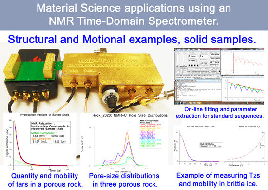
Featured Application

This compact but precision highly stable NMR time-domain relaxation spectrometer is most useful for quantitative material science measurements of both the mass and the mobility/dynamics/stiffness/viscosity/rigidity of hydrocarbons and polymers, both in the bulk and in sub-nano-meter and upward sized pores. It is highly useful for studying the properties of hydrocarbons in pores in applications such as recovered porous rock samples from oil reservoirs, and in fired biochar porous carbon samples, to give just two examples. In addition, applicable to both these fields of study is the ability to make NMR Cryoporometric measurements of pore-size distributions in porous materials, for sub-nano- to over micrometer sized pores.

Abstract

NMR Relaxation (NMRR) is an extremely useful quantitative technique for material science, particularly for studying polymers and porous materials. NMR Cryoporometry (NMRC) is a powerful technique for the measurement of pore-size distributions and total porosities. This paper discusses the use, capabilities and application of a newly available compact NMR time-domain relaxation spectrometer, the Lab-Tools Mk3 NMR Relaxometer & Cryoporometer [Lab-Tools (nano-science), Ramsgate, Kent, UK (2019)]. Being Field Programmable Gate Array based means that it is unusually compact, which makes it particularly suitable for the lab bench-top, in the field and also mobile use. Its use with a variable-temperature NMR probe such as the Lab-Tools Peltier thermo-electrically cooled variable-temperature (V-T) probe is also discussed. This enables the NMRC measurement of pore-size distributions in porous materials, from sub-nano- to over 1 micron sized pores. These techniques are suitable for a wide range of porous materials and also polymers. This instrument comes with a Graphical User Interface (GUI) for control, which also enables both online and offline analysis of the measured data. This makes it is easy to use for material science studies both in the field and in university, research institute, company and even school laboratories. The Peltier cooling gives the precision temperature control and smoothness needed by NMR Cryoporometry, particularly near the probe liquid bulk melting point. Results from example NMR Relaxation and NMR Cryoporometric measurements are given.
PACS:
J0101; 07.57.Pt; 07.50.Ek; 07.05.-t; 07.05.Fb; 07.05.Hd; 84.30.-r; 84.30.Le; 84.30.Sk; 85.40.Bh

Graphical Abstract

1. Introduction

NMR Relaxation (NMRR) is an extremely useful quantitative technique for material science, particularly for studying polymers and porous materials [1,2,3,4,5,6,7,8,9,10,11,12,13]. The measurement of NMR relaxation amplitudes and decay times enables the measurement of both the mass and qualities which are variously described as mobility, dynamics, stiffness, viscosity or rigidity, for hydrocarbons and polymers, both in the bulk and in pores, Section 4.
NMR relaxation can be used directly to measure micron-sized pore-sizes [11,14,15,16], provided one knows the surface relaxation properties of the porous material [12,17]—often termed NMR Relaxometry. NMR Relaxometry is of limited use for nano-metric sized pores. Alternatively, NMR Cryoporometry (NMRC) [10,18,19,20] is a powerful technique for the measurement of nano-metric pore-size distributions and total porosities, based on the lowered melting temperature of liquids in the pores—the Gibbs–Thomson effect [18,21,22,23], Section 3.2.
This paper discusses the use and application of the Lab-Tools Mk3 precision compact NMR time-domain spectrometer for both NMRR, Section 3.1 and Section 4, and NMRC, Section 3.2 and Section 5.
This NMR spectrometer is based on a Field Programmable Gate Array (FPGA). Other examples of FPGA based instruments appear in the literature, for instance [24,25,26], but do not appear to be such rather compact and yet complete and easy to use NMR time-domain spectrometers. This instrument is an NMR time-domain spectrometer that auto-tunes and is immediately ready for research measurements, under control of a Graphical User Interface (GUI). Data fitting and parameter extraction is performed online during the measurements, and can also be performed offline using the same Graphical User Interface or another copy elsewhere.
A particular feature of this spectrometer is that it is fast recovery and so can measure NMR Relaxation both in the bulk and in sub-nano-meter and upward sized pores, for materials that may be liquid, gel, waxy, tarry … [13], and an example is given of it measuring T 2 s in brittle ice (and hence the mobility of the ice molecules), see Figure 1 and Figure 2.
This is highly useful for studying the properties of hydrocarbons in both recovered porous rock samples from oil reservoirs, and in fired biochar porous carbon samples, for example [27].
A more detailed discussion of NMR Relaxation, and specific application examples, are given in Section 4.
Some applications of the Lab-Tools Peltier thermo-electrically cooled variable–temperature (V–T) probe [28,29] are also discussed, Section 2.1, which enables this spectrometer to make NMRC measurements of pore-size distributions in porous materials on the unusually wide pore scale range of sub 1 nm to over one micron [18]. Specific application examples are discussed in detail, Section 5.
All of these techniques are suitable for a wide range of polymers [18,20] and porous materials [18], including porous glass [30,31], zeolites [32], cement [33], clays [18], rock [27,34], wood [35], and biochar and other porous carbons [18,27,36,37]. In polymers, crystalline/amorphous ratios may be measured. By swelling rubbers and polymers by adding liquids to them, cross-link density and nano- to micro-porous properties of the polymer may be obtained [18,20,38]. In biochar, progressive changes to the quantity and mobility of hydrocarbons, as well as changes in pore-blocking, as a function of preparation temperature, have been demonstrated [27].
All these measurement techniques can be implemented using this recently developed highly compact Spectrometer, based on a Field Programmable Gate array (FPGA) module and custom surface mount low-noise NMR receiver and NMR linear transmitter. This instrument has a high proportion of the R.F. circuitry in a digital form, implemented as firmware in the FPGA, which aids long-term stability. The FPGA module is credit-card sized, and the NMR receiver and NMR transmitter are each even smaller. Complete with a Graphical User Interface (GUI) for control and online and offline analysis, this instrument has been found to be particularly suitable for material science studies.

2. Apparatus

A recently released time-domain NMR relaxation spectrometer [MK3 NMR Spectrometer, Lab-Tools Ltd. (nano-science), Ramsgate, Kent, UK, 2019] [39] and associated Peltier thermo-electrically cooled variable-temperature NMR probe [Mk3 NMR Cryoporometer, Lab-Tools, Ramsgate, Kent, UK] [40], Figure 3, were used to conduct a number of experiments, to evaluate their suitability for material-science experiments.
This spectrometer is built around a credit-card sized Field Programmable Gate Array Red Pitaya module [41] for the digital RF, with custom firmware, C and array processing AplX programs added, and with attached custom surface mount low-noise receiver and linear transmitter.
The signal-to-noise (S/N) appears to be good, see Figure 4. A number of important parameters of the NMR spectrometer were evaluated, as part of the process to determine what experiments might be feasible, see Section 6.

2.1. Temperature Measurement and Control

There are many NMR material science experiments which are far more informative if carried out as a function of temperature. In particular, highly useful NMR T 1 and T 2 minima measurements may then be made, which provide additional information on the motional dynamics in the sample. NMR Cryoporometry also ideally needs very well controlled wide-range temperature ramps (typically from ~100 K to ~350 K). The temperature measurement needs to reflect as true a temperature measurement of the sample as possible, and this apparatus appears to give a precision better than 10 mK [28,29]. To aid this precision, “sample” and “control” copper-constantan thermocouples were used, the control thermocouple offering a faster thermal response time for dynamic control purposes, while the sample thermocouple offers longer term precision, being in very close contact with the sample.
Two different 0C thermocouple junction references have been used in this work:
  • Referenced to a cell of distilled water maintained half frozen (Omega IceCell Model TRCIII), with a third thermocouple attached to a thermal mass in a Dewar provided a short-term temperature reference to help reduce the effect of the temperature cycling in the IceCell.
  • Electronic diode junction 0C references have in recent years improved greatly, and these are under evaluation. They have the advantage of no temperature cycling.
These thermal EMFs were measured and averaged using a USB interfaced 5 channel, 24 bit Digital Volt Meter (DVM, Lab-Tools, Ramsgate, Kent, UK). During each measurement of NMR signal amplitude, the DVM measurements were further averaged. Thermal EMFs were converted to temperature using a 18 segment quadratic piece-wise polynomial algorithm, with segments contiguous in amplitude and gradient. The agreement with the original NIST thermocouple data are believed to be good to better than 1 mK [42].
The Peltier cooling offers extreme uniformity of warming rate needed by NMR Cryoporometry, particularly near the probe liquid bulk melting point, as well as the ability to have temperature ramps that last over days. NMRC measurement of pore diameters in excess of 1 micron were measured, with acceptable repeatability at 1 micron pore diameter.

3. Key Time-Domain NMR Methods

3.1. Nuclear Magnetic Resonance Relaxation (NMRR) for Material Science

NMRR is an extremely useful quantitative technique for material science, particularly applicable to polymers and porous materials. A powerful RF pulse (a π /2 pulse) at the NMR resonant frequency may be used to tip the equilibrium nuclear magnetization of certain nuclei such as hydrogen into the transverse plane. There it precesses at the resonant RF frequency, generating an exceedingly small RF signal that may be amplified and detected.
The initial amplitude of the NMR signal—the Free Induction Decay (FID)—gives a robust quantitative measure of the amount of material in the sample; to obtain a mass calibrated measurement, it is necessary to also make measurements on one or more calibration samples of known weight that ideally should be similar to the expected liquid, polymer or hydrocarbon. The amplitude of the FID decays at a rate at least partly determined by the dipole–dipole interactions between the nuclei—dipolar broadening—the adjacent nuclei alter the local magnetic field at a given nucleus, resulting in a short, often Gaussian-like T 2 decay. A short transverse or dipolar decay time of around 10 μ s is characteristic for a very rigid material like ice. If there is motion of the nuclei, this can cause an averaging of this effect, so that the decay can become slower, and can then tend to be approximately an exponential. This is typical for say a tar, with T 2 s perhaps between 20 μ s to 100 μ s. However, as T 2 gets longer due to motional narrowing, the FID decay time is then often limited by local field variation such as the homogeneity of the magnet, or sometimes by inhomogeneities in the sample (which may be porous), and the FID decays at a rate characterised as T 2 *. This is then typical of a soft material such as a polymer or say a candle wax.
This is not the end of the story, however, as the dephased magnetisation can often then be re-focussed by applying a chain of re-focussing NMR pulses, such as the Car–Purcell–Meiboom–Gill (CPMG) sequence, to obtain a chain of NMR echoes, whose peak amplitudes then trace out the true T 2 decay. These longer true T 2 times are then typical of the above polymers or candle wax, and are often around a few milli-seconds, or can be as long as seconds, typical of a mobile liquid. Organic molecules frequently exhibit reptation, which often result in a non- or multi- exponential signal decay. The decays may also be multi-component when both crystalline and amorphous components are present in a polymer.
Finally, we need to consider the time for the magnetisation to re-equilibrate with the “lattice” (the longitudinal decay time T 1 ). T 1 is often long (many seconds) for rigid materials but reduces and becomes equal to the true T 2 time for a mobile liquid like water. It can thus be seen that the NMR FID, T 2 * and true T 2 may give information on the sample that for different applications is variously characterised as mobility, dynamics, stiffness, viscosity or rigidity. These are highly useful parameters, rapidly providing data on the physical state of the sample as a function of local condition and sample temperature [1,2,3].

NMRR for Determining Mass and Mobility of Hydrocarbons in Porous Materials

Many porous materials, such as recovered porous rocks, or fired carbons such as biochar, contain hydrocarbons in the pores. As well as the hydrocarbon mass, the dynamical information may also be obtained as above from the NMR decay. For hydrocarbons that are fairly rigid, like tars or some polymers, the FID decays rapidly, and information on the mobility may be obtained directly from the T 2 of the FID, which may be multi-component [27], and also see Section 4. Other samples may also contain more mobile components such as light oils that then need an NMR pulse sequence chain such as the Carr–Purcell–Meiboom–Gill (CPMG) sequence to recover the dynamical information, often multi-component.

3.2. NMR Cryoporometry

3.2.1. NMRC History

Originating in 1993 at the University of Kent, NMR Cryoporometry (NMRC) [43] is now an important method for determining pore sizes in porous media.
Josiah Willward Gibbs, James Thomson, his brother WilliamThomson (later Lord Kelvin), and J. J. Thomson were the pioneers of the theory behind phase transitions for confined materials. They applied experiment, thermodynamics and generalised dynamics to produce equations that well describe the phase-change behaviour of liquids in confined geometry [44,45,46,47]. The Gibbs–Thomson equation is the constant pressure version of the Gibbs Equations [21,22,23], whereas the Kelvin equation [46] is the constant temperature version.

3.2.2. NMRC Theory

A development of the Gibbs–Thomson equation has been discussed [18,48,49] that relates these phase changes so that the pore area a p and volume v p are related to the melting point depression
Δ T m = T m T m ( x ) a p v p · σ s l T m cos ( φ ) Δ H f ρ s k d σ s l T m x Δ H f ρ s
For many purposes, this may be simplified so that the pore diameter x {Å} is related to a melting point depression {K}by
Δ T m = k G T / x
where we are grouping all the thermodynamic terms into a single constant, k G T {K.Å}, the Gibbs– Thomson coefficient—usually established by an experiment.
It is important to note that k G T includes a term dependent on pore geometry, as does the Kelvin equation. k d is the geometry term, and is equal to four for a spherical liquid-crystalline interface (conventionally assumed for cylindrical pores). T m is the bulk melting point and the other terms are thermodynamic and density terms [49,50].
The measurement of the pore volume vs. size distributions is facilitated by differentiating and re-mapping the melting curve data using the Rahman–Strange transformation:
d v d x = k G T x 2 · d v d T .
In Figure 5, the Gibbs–Thomson Coefficients k G T are calculated from the slopes of the plotted lines of melting point depression vs. inverse nominal pore diameter [50].

3.2.3. NMRC Protocol

The protocol of an NMR Cryoporometry experiment involves absorbing a liquid into pores; freezing the liquid, and then warming the sample. The NMR echo amplitude is monitored, so as to determine the amount of liquid that has melted as a function of temperature. This gives a measure of the pore volume vs. melting temperature, and hence, via the Gibbs–Thomson equation, the pore size distribution.
The NMR measurement required is very simple, just a [ π / 2 τ π τ Echo] NMR sequence, with the echo at an NMR 2 τ measuring time of typically 500 μ s to 20 ms, so as to avoid any signal from solid ice. The amplitude of the NMR Echo is recorded as a function of temperature. The Echo is polynomial fitted, and the polynomial solved to determine the peak amplitude. We can then apply the Gibbs–Thomson equation and the Rahman–Strange transformation to obtain the pore volume distributions, as a function of pore diameter.
A recent calibration is frequently employed, as appropriate to water in Sol-Gel silica, at an NMR 2 τ measuring time of 2 ms [50]:
k G T = 580 K . Å

4. NMR Relaxation Results Obtained Using the Spectrometer and Peltier Cooled Probe

4.1. Nuclear Magnetic Resonance Relaxation for Determining Mass and Mobility of Hydrocarbons in Porous Materials

A sample of Barnett shale was measured by NMR Relaxation (NMRR) to obtain an estimate of the quantity and mobility of the hydrocarbons in the pores. Measuring tarry materials in rock pores is not an easy measurement for NMR spectrometers, as the rock material gives a fast decay (extremely broad-line, in spectroscopic terms), due to the dipole–dipole interactions with the rock, and the quantities are small—the total sample is only a couple of 10s of milli-gram, and the organic components resolved are in the 10 s to 100 s of micrograms.
Figure 6 shows a two component fit to hydrocarbons in the porous rock sample. Any residual signal from an empty probe has been subtracted. Both components are exponentials that are not immediately visible to the eye; however, if the longer exponential component is subtracted from the measured data, and the resultant plotted logarithmically, Figure 7, a flat baseline is obtained, with a straight-line residual at shorter times. This appears to be very convincing evidence for a double exponential decay for the FIDS for the hydrocarbons in these pores, which provides important information regarding the mobility and dynamical processes in these samples.
In the logarithmic plot, the linearity of the baseline and the fitted short-component, following subtraction of the baseline, are also convincing evidence for the linearity of the NMR receiver and the overall quality of the measured time-domain data, including good signal-to-noise.

4.2. Bulk Ice T 2 Measurement

Using the Peltier cooled variable-temperature probe, the Free Induction Decays (FIDs) for bulk brittle ice were measured, from below −20 C to −2 C. As expected, a Gaussian curve was the preferred fit for all the data sets; the automated fitting routine with initial linearised fit, followed by a full nonlinear fit, was used to extract the amplitudes and relaxation times as before.
Four example measurements at −20 C, −15 C, −10 C and −5 C are shown in Figure 1. These have all been Boltzmann corrected, to take into account the amplitude changes as a function of temperature [51].
It requires a fairly fast recovery NMR spectrometer to measure these FIDs in brittle ice. This linear NMR transmitter does not have the power of the Lab-Tools digital NMR transmitter (still at the proto-type stage), but can still generate an RF B 1 of about 1 mT in a 5 mm OD NMR sample tube (just under a 6 μ s π / 2 NMR pulse). These brittle ice FIDs were measured using the variable-temperature (NMR Cryoporometric) probe, with a 3 mm OD NMR sample. Due to the constraints of a probe optimised for Cryoporometry, this generates a lower RF B 1 of about 0.7 mT (about a 9 μ s π / 2 NMR pulse).
Measuring the Ice FIDs, from the middle of the NMR pulse (necessary to correctly fit a Gaussian), the first 4.5 μ s are occupied by the NMR transmit pulse, and about the next 3 μ s are the probe ring-down and receiver recovery. Thus, with the decimation set to full band-width, and the integral count set to 2, so as to reduce ringing from the decimation filter, then the recovered signal is fully usable at 7.5 μ s from the centre of the pulse. This recovery performance is achieved because the probe is designed deliberately to be broadband, with about a 1 MHz bandwidth. This also has the advantage of making the tuning of the probe insensitive to sample changes, such as the freezing or melting of a liquid sample, or very wide probe temperature changes.
The measured Gaussian T 2 s were plotted as a function of temperature, and a polynomial curve fitted to them, Figure 2.

5. NMR Cryoporometric Results Obtained Using the Spectrometer and Peltier Cooled Probe

The NMR Cryoporometry measurements were performed on a purpose built NMR Scanning Cryoporometer based on the above spectrometer, with Mk3 Peltier thermo-electrically cooled probe.

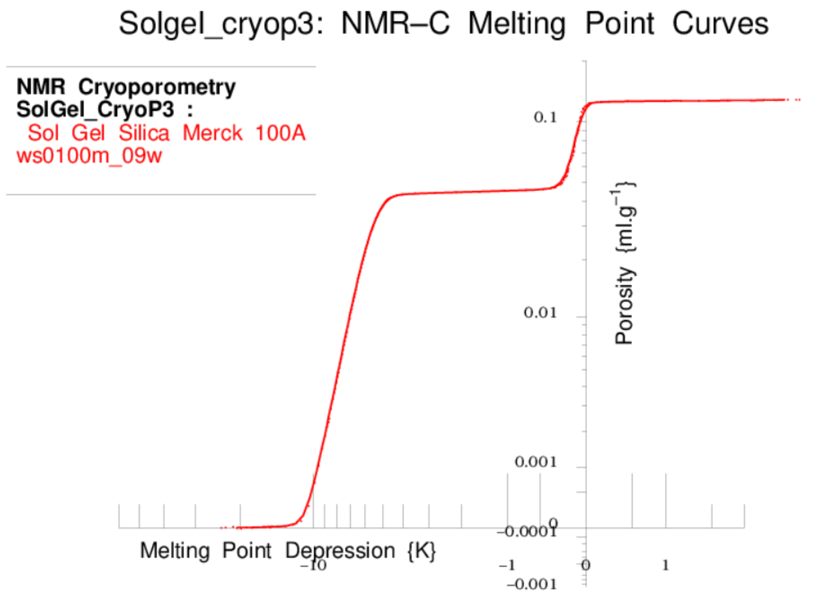
5.1. NMR Cryoporometric Measurement on a Sol-Gel Silica

A Sol-Gel silica of nominal pore diameter of 100 Å (as determined by gas adsorption) was measured using the NMR Cryoporometer, with distilled water as the probe liquid. The samples were prepared in 3 mm glass NMR tubes, and dried at 120 °C overnight. The small diameter of the tubes assists with the sample all being iso-thermal. Weighing was performed so that the masses of all the dry solid and added liquid were known.
For this set of results, a recent calibration was employed, as appropriate to water at an NMR 2 τ measuring time of 2 ms [50]:
k G T = 580 K . Å
At low temperatures (Figure 8), the water is all frozen, and at a 2 τ measuring time of 2 ms gives a negligible signal, due to the short T 2 of the brittle ice. Between about −10 °C and −5 °C, the liquid in the pores melts, to then give a plateau between about −5 °C to −1 °C, followed by another rise in signal amplitude near 0 °C as the bulk liquid around the grains melts. This final plateau gives a pore–volume calibration to the whole measurement, as the mass of this liquid has been measured.
The signal-to noise was excellent, as can be seen on the following melting curve, Figure 9, for 23 mg of water over-filling 21 mg of sol-gel silica. The measurement points are mostly hidden under the fitted red curve, as can be seen using a bi-symmetric log plot [52]. These plots are helpful in determining that at the lowest temperature all the liquid has frozen, so as to obtain an accurate NMRC pore-size distribution, particularly at low pore-size values. The resultant pore-size distribution is shown in Figure 10.

5.2. NMR Cryoporometric Measurements on Three Porous Rocks

Pore-size distribution data have been measured on three porous rocks using this Cryoporometer, on a Sandstone, Carbonate and Barnett Shale porous rock, Figure 11. The data show reasonable agreement between repeated runs, particularly considering that the pore-size distributions are, as per the Rahman–Strange transformation, the differential of the measured melting point curves. It should be noted that, while sandstone pore-size distribution data are obtainable by other techniques, such as Relaxometry, private discussion has indicated that NMR Cryoporometry is perhaps one of the most robust techniques for small pore data in carbonate and shale samples.

5.3. NMR Cryoporometric Measurements on Four Biochar Samples with Different Processing

Some data were measured on four biochar samples using the prototype of this Cryoporometer [37]. The biochar was derived from oilseed rape (OSR) and mixed softwood pellets (SWP) containing 5:95 pine:spruce, from the United Kingdom Biochar Research Centre (UKBRC) Edinburgh. It was pyrolyzed in a pilot-scale rotary kiln unit, at 550 °C and 700 °C, Figure 12.

6. Measured Instrument Parameters and Capabilities

A number of important parameters of the NMR spectrometer were also evaluated, as part of the above measurement process:
  • System signal-to-noise: The controlling Graphical User Interface (GUI) configures the NMR data capture to start before the first NMR pulse, and this signal provides both a data base-line and uncontaminated signal that the instrument uses to measure the base noise-level, for each trace. A typical signal at the demodulated receiver output is shown in Figure 4. Measured noise levels appear to be around 1 mV RMS (for a typical 0.5 V signal) so a Signal-to-Noise (S/N) of about 500 for a typical 25 mg water sample in the 3 mm probe), for a signal filter setting of 250 kHz and 5 point integral filter (suitable for a typical NMR Free Induction Decay (FID) and Echo experiment with a liquid)—thus, an RMS noise level, single shot, equivalent to about 50 μ g for water. When conducting NMR Cryoporometric experiments, a slow warming ramp is needed so that all the sample is as isothermal as possible, and thus averaging times of 100 to 300 s per captured point were commonly employed. The NMR echo is fitted with a polynomial, and the polynomial solved to obtain a peak amplitude. This gave RMS noise levels for the averaged NMR Cryoporometric signal of around 50 to 100 μ V, so an S/N of about 5000 to 10,000 for typical 3 mm samples containing about 25 mg of water. This gives a very useful dynamic range to the resultant pore-size distributions, see Figure 9, the data for which appears to indicate the RMS sensitivity in a typical NMRC measurement to be around 15 nl of porosity. This is particularly important for low porosity samples.
  • NMR RF Pulse Power: For this spectrometer, the linear RF transmitter amplifier delivers a π /2 pulse into the supplied room-temperature NMR probe (5 mm OD standard NMR tube) of about 6 μ s, while, for the NMR Cryoporometric probe with a 3 mm OD NMR sample, it is about 9 μ s.
  • Recovery time after the NMR Pulse: The time from the middle of the RF pulse to the first usable signal is a key feature for spectrometers when measuring more rigid materials such as solid polymers, waxes, tars, etc. With the receiver set to full bandwidth and 2 point integration (to suppress filter ringing), the system appears to recover pleasingly quickly, even for the Cryoporometric probe, with an overall time from the centre of the NMR pulse being no greater than 7 or 8 μ s. This enabled the measurement of FIDs from materials as rigid as bulk ice, see Section 4.2.
  • Portability: A significant feature of this Field Programmable Gate Array (FPGA) based equipment is its compactness, which might make it suitable for use in the field or even for mobile use. As such applications are still to be evaluated, these measurements having been conducted on the laboratory bench-top. For mobile use, more compact non-mains power supplies will be needed.

7. Conclusions and Suggestions

This spectrometer [39] is a highly versatile instrument and is very convenient for a range of uses for material science. Since much of the RF analysis is digital, it exhibits excellent long term stability, which is particularly important for NMR cryoporometry. The addition of the Peltier thermo-electrically cooled probe makes it very applicable to NMR experiments that require the sample temperature to be changed, including the measurement of NMR Cryoporometric pore-size distributions [40]. This variable-temperature probe is particularly appropriate to long duration experiments, which may sometimes last for days.

7.1. Diffusion and Controlled Magnetic Field Gradient Experiments

An important step forward in the range of experiments that could be carried out would be adding the ability to measure diffusion and pore connectivity by a number of techniques. This can be done most simply with little extra complexity by making measurements in the fringe field of a permanent or superconducting magnet [53,54]. However, adding the ability to modify the magnetic gradient in the sample using constant current gradients or gradient pulses [51,55,56,57] or sine-waves [58] are also powerful techniques. While the pulse techniques may significantly increase the apparatus complexity, the stability of this spectrometer should act as a suitable platform on which to make these additions.

7.2. Portability

Clearly, while the pictured 24 MHz magnet (Figure 3) is carriable, this does not make for a particularly portable system. An important future step for this time-domain NMR system could be the addition of a single-sided NMR magnet—“NMR Mouse” [59], so as to make a completely human-portable NMR system that could be taken to samples in the field and used in a freely un-tethered mobile fashion.

8. Patents

Webber, Patent No.: US 9,810,750 B2, Nov 7th2017. Nuclear Magnetic Resonance Probes. Application No.: 14/316,409 Filed: 26 Jun. 2014. John Beausire Wyatt Webber. Ramsgate (GB).

Funding

This research received no external funding, and the Mk3 NMR spectrometer and variable-temperature probe has been developed using Lab-Tools’ resources.

Acknowledgments

The Xilinx firmware in the Red Pitaye FPGA module for the pulsed NMR spectrometer was developed and written by Pavel Demin, Louvain-la-Neuve, Belgium [60].

Conflicts of Interest

The author declares no conflict of interest.

Abbreviations

The following abbreviations are used in this manuscript:
NMRNuclear Magnetic Resonance
NMRRNuclear Magnetic Resonance Relaxation
NMRCNuclear Magnetic Resonance Cryoporometry
FIDFree Induction Decay
CPMGCarr–Purcell–Meiboom–Gill (NMR sequence)
T 1 Longitudinal Relaxation time—Time for NMR spins to equilibrate with the lattice
T 2 Transverse Relaxation time—Time for NMR spins to inter-equilibrate with each other
T 1 ρ T1 in the Rotating Frame
k G T Gibbs–Thomson coefficient
V-TVariable-Temperature
RFRadio Frequency
EMFElectro-Motive-Force—voltage
CPUCentral Processing Unit
ADCAnalogue to Digital Convertor
DACDigital to Analogue Convertor
DVMDigital Volt Meter
FPGAField Programmable Gate Array
ODOutside Diameter
3DThree-Dimensional
Mk3Mark 3
NIST(USA) National Institute of Science and Technology
MDPIMultidisciplinary Digital Publishing Institute
DOAJDirectory of Open Access Journals

References

  1. Abragam, A. The Principles of Nuclear Magnetism; Clarendon Press: Oxford, UK, 1961; Available online: https://books.google.co.uk/books/about/The_Principles_of_Nuclear_Magnetism.html?id=9M8U_JK7K54C (accessed on 14 April 2020).
  2. Denise Besghini, M.M.; Simonutti, R. Time Domain NMR in Polymer Science: From the Laboratory to the Industry. Appl. Sci. 2019, 9, 1801. [Google Scholar] [CrossRef] [Green Version]
  3. Fabian Vaca Chavez, K.S. Time-Domain NMR Observation of Entangled Polymer Dynamics: Universal Behavior of Flexible Homopolymers and Applicability of the Tube Model. Macromolecules 2011, 44, 1549–1559. [Google Scholar] [CrossRef]
  4. Todt, H.; Guthausen, G.; Burk, W.; Schmalbein, D.; Kamlowski, A. Water/moisture and fat analysis by time-domain NMR. Food Chem. 2006, 96, 436–440. [Google Scholar] [CrossRef]
  5. Brownstein, K.; Tarr, C. Importance of classical diffusion in NMR studies of water in biological cells. Phys. Rev. A. 1979, 19, 2446–2453. [Google Scholar] [CrossRef]
  6. Gladden, L. Nuclear-magnetic-resonance studies of porous-media. Chem. Eng. Res. Des. 1993, 71, 657–674. [Google Scholar]
  7. Callaghan, P.; Godefroy, S.; Ryland, B. Diffusion-relaxation correlation in simple pore structures. J. Magn. Reson. 2003, 162, 320–327. [Google Scholar] [CrossRef]
  8. Fantazzini, P.; Brown, R.; Borgia, G. Bone tissue and porous media: Common features and differences studied by NMR relaxation. Magn. Reson. Imaging 2003, 21, 227–234. [Google Scholar] [CrossRef]
  9. Kimmich, R.; Fatkullin, N.; Mattea, C.; Fischer, E. Polymer chain dynamics under nanoscopic confinements. Magn. Reson. Imaging 2005, 23, 191–196. [Google Scholar] [CrossRef]
  10. Hansen, E.; Fonnum, G.; Weng, E. Pore morphology of porous polymer particles probed by NMR relaxometry and NMR cryoporometry. J. Phys. Chem. 2005, 109, 24295–24303. [Google Scholar] [CrossRef]
  11. McDonald, P.J.; Mitchell, J.; Mulheron, M.; Aptaker, P.S.; Korb, J.P.; Monteilhet, L. Two-dimensional correlation relaxometry studies of cement pastes performed using a new one-sided NMR magnet. Cem. Concr. Res. 2007, 37, 303–309. [Google Scholar] [CrossRef]
  12. D’Agostino, C.; Mitchell, J.; Mantle, M.D.; Gladden, L.F. Interpretation of NMR Relaxation as a Tool for Characterising the Adsorption Strength of Liquids inside Porous Materials. Chemistry 2014, 20, 13009–13015. [Google Scholar] [CrossRef] [PubMed] [Green Version]
  13. Webber, J.B.W. Biological, Medical and Nano Structured materials—NMR done Simply. Arch. Biomed. Eng. Biotechnol. 2019, 1. [Google Scholar] [CrossRef] [Green Version]
  14. Prado, P.; Balcom, B.; Beyea, S.; Bremner, T.; Armstrong, R.; Pishe, R.; Gratten-Bellew, P. Spatially resolved relaxometry and pore size distribution by single-point MRI methods: Porous media calorimetry. J. Phys. D Appl. Phys. 1998, 31, 2040–2050. [Google Scholar] [CrossRef]
  15. Friedemann, K.; Schoenfelder, W.; Stallmach, F.; Kaerger, J. NMR relaxometry during internal curing of Portland cements by lightweight aggregates. Mater. Struct. 2008, 41, 1647–1655. [Google Scholar] [CrossRef]
  16. Schoenfelder, W.; Glaeser, H.R.; Mitreiter, I.; Stallmach, F. Two-dimensional NMR relaxometry study of pore space characteristics of carbonate rocks from a Permian aquifer. J. Appl. Geophys. 2008, 65, 21–29. [Google Scholar] [CrossRef]
  17. Strange, J.; Mitchell, J.; Webber, J. Pore surface exploration by NMR. Magn. Reson. Imaging 2003, 21, 221–226. [Google Scholar] [CrossRef] [Green Version]
  18. Mitchell, J.; Webber, J.; Strange, J. Nuclear magnetic resonance cryoporometry. Phys. Rep. 2008, 461, 1–36. [Google Scholar] [CrossRef] [Green Version]
  19. Petrov, O.V.; Furo, I. NMR cryoporometry: Principles, applications and potential. Prog. Nucl. Magn. Res. Spectrosc. 2009, 54, 97–122. [Google Scholar] [CrossRef]
  20. Rottreau, T.J.; Parkes, G.E.; Schirru, M.; Harries, J.L.; Mesa, M.G.; Topham, P.D.; Evans, R. NMR Cryoporometry of Polymers: Cross-linking, Porosity and the Importance of Probe Liquid. Colloids Surf. A Physicochem. Eng. Asp. 2019, 575, 256–263. [Google Scholar] [CrossRef]
  21. Gibbs, J. Collected Works; Longmans, Green and Co.: New York, NY, USA, 1928. [Google Scholar]
  22. Gibbs, J. The Scientific Papers of J. Willward Gibbs; New Dover ed.; Volume 1: Thermodynamics; Dover Publications, Inc., Constable and Co.: New York, NY, USA; London, UK, 1906. [Google Scholar]
  23. Gibbs, J. On the equilibrium of hetrogeneous substances. Trans. Conn. Acad. 1878, 96, 441–458. [Google Scholar]
  24. Belmonte, S.B.; Sarthour, R.S.; Oliveira, I.S.; Guimaes, A.P. A field-programmable gate-array-based high-resolution pulse programmer. Meas. Sci. Technol. 2003, 14, N1. [Google Scholar] [CrossRef]
  25. Hemnani, P.; Rajarajan, A.; Joshi, G.; Ravindranath, S. FPGA Based RF Pulse Generator for NQR/NMR Spectrometer. Procedia Comput. Sci. 2016, 93, 161–168. [Google Scholar] [CrossRef]
  26. Takeda, K. A highly integrated FPGA-based nuclear magnetic resonance spectrometer. Rev. Sci. Instrum. 2007, 78, 033103. [Google Scholar] [CrossRef] [PubMed]
  27. Webber, J.B.W.; Corbett, P.; Semple, K.T.; Ogbonnaya, U.; Teel, W.S.; Masiello, C.A.; Fisher, Q.J.; Valenza, J.J., II; Song, Y.Q.; Hu, Q. An NMR study of porous rock and biochar containing organic material. Microporous Mesoporous Mater. 2013, 178, 94–98. [Google Scholar] [CrossRef]
  28. Webber, J.B.W. Thermostatted NMR Probe. EU Patent EP2818885, 26 June 2014. [Google Scholar]
  29. Webber, J.B.W. Nuclear Magnetic Resonance Probes. U.S. Patent 9,810,750 B2, 7 November 2017. [Google Scholar]
  30. Webber, J.; Strange, J.; Dore, J. An evaluation of NMR cryoporometry, density measurement and neutron scattering methods of pore characterisation. Magn. Reson. Imaging 2001, 19, 395–399. [Google Scholar] [CrossRef] [Green Version]
  31. Webber, J.B.W. Accessible Catalyst Pore Volumes, for Water and Organic Liquids, as probed by NMR Cryoporometry. Diffusion-fundamentals.org 2014, 22, 1–8. [Google Scholar]
  32. Andreev, A.S.; Beau Webber, P.S. Advanced NMR for Industrial Applications: Structure, Porosity, and Acidity; Characterization of Catalytic Materials through a Facile Approach to Probe OH Groups; Total Research and Technology Feluy (TRTF), Lab-Tools Ltd.: Ramsgate, UK, 2019. [Google Scholar]
  33. Boguszynska, J.; Tritt-Goc, J. H-1 NMR cryoporometry study of the melting behavior of water in white cement. Z. Naturforsch. Sect. A J. Phys. Sci. 2004, 59, 550–558. [Google Scholar] [CrossRef]
  34. Fleury, M.; Fabre, R.; Webber, J.W. Comparison of Pore Size Distribution by NMR Relaxation and NMR Cryoporometry in Shales. In Proceedings of the International Symposium of the Society of Core Analysts, St. John’s, NL, Canada, 16–21 August 2015. [Google Scholar]
  35. Ankathi, S.K.; Zhou, W.; Webber, J.B.; Patil, R.; Chaudhari, U.; Shonnard, D. Synergistic Effects between Hydrolysis Time and Microporous Structure in Poplar. ACS Sustain. Chem. Eng. 2019, 7, 12920–12929. [Google Scholar] [CrossRef]
  36. Aditya Rawal, S.D.J.; Webber, J.B.W. Mineral-Biochar Composites: Molecular Structure and Porosity. Environ. Sci. Technol. 2016, 50, 7706–7714. [Google Scholar] [CrossRef] [Green Version]
  37. Wong, J.; Webber, J.; Ogbonnaya, U. Characteristics of biochar porosity by NMR and study of ammonium ion adsorption. J. Anal. Appl. Pyrolysis 2019, 143, 104687. [Google Scholar] [CrossRef]
  38. Strange, J.; Webber, J. Characterization of Porous Solids by NMR. In Proceedings of the 12th Specialized Colloque Ampere, Corfu, Greece, 10–15 September 1995. [Google Scholar]
  39. Webber, J.B.W. Lab-Tools Mk3 NMR Relaxometer, Lab-Tools (Nano-Science); Ramsgate: Kent, UK, 2019. [Google Scholar]
  40. Webber, J.B.W. Lab-Tools Mk3 NMR Cryoporometer, Lab-Tools (Nano-Science); Ramsgate: Kent, UK, 2019. [Google Scholar]
  41. Red Pitaya FPGA Module. Available online: www.redpitaya.com (accessed on 16 February 2019).
  42. Meyer, C.W.; Garrity, K.M. Updated uncertainty budgets for NIST thermocouple calibrations. In Proceedings of the AIP Conference Proceedings, Physical Measurement Laboratory/Sensor Science Division, Thermodynamic Metrology Group, Los Angeles, CA, USA, 19–23 March 2012; p. 1552. [Google Scholar] [CrossRef] [Green Version]
  43. Strange, J.H.; Rahman, M.; Smith, E.G. Characterization of Porous Solids By Nmr. Phys. Rev. Lett. 1993, 71, 3589–3591. [Google Scholar] [CrossRef] [PubMed]
  44. Thomson, J. On Crystallization and Liquefaction, as influenced by Stresses tending to change form in the Crystals. Proc. R. Soc. 1862, xi, 473–481. [Google Scholar]
  45. Thomson, J. Theoretical Considerations on the Effect of Pressure in Lowering the Freezing Point of Water. Trans. R. Soc. 1849, xvi, 575–580. [Google Scholar] [CrossRef] [Green Version]
  46. Thomson, W. On the Equilibrium of Vapour at a Curved Surface of Liquid. Philos. Mag. 1871, 42, 448–452. [Google Scholar] [CrossRef]
  47. Thomson, J. Application of dynamics to Physics and Chemistry; Macmillan & Co: London, UK, 1888. [Google Scholar]
  48. Webber, J. A generalisation of the thermoporisimetry Gibbs–Thomson equation for arbitrary pore geometry. Magn. Reson. Imaging 2003, 21, 428. [Google Scholar] [CrossRef]
  49. Webber, J. The dimensional term in the Gibbs–Thomson equation, describing the behaviour of liquids in porous media, is being investigated by NMR relaxation, novel protocol NMR cryoporometry, neutron scattering and ab initio QM-MD simulation. Magn. Reson. Imaging 2006, 25, 589–590. [Google Scholar] [CrossRef]
  50. Webber, J.B.W. Studies of nano-structured liquids in confined geometry and at surfaces. Prog. Nucl. Magn. Res. Spectrosc. 2010, 56, 78–93. [Google Scholar] [CrossRef] [Green Version]
  51. Webber, J.B.W. The Characterisation of Porous Media. Ph.D. Thesis, Physics, University of Kent, Canterbury, UK, 2000. [Google Scholar]
  52. Webber, J.B.W. A bi-symmetric log transformation for wide-range data. Meas. Sci. Technol. 2013, 24, 027001. [Google Scholar] [CrossRef] [Green Version]
  53. Carlton, K.J.; Halse, M.R.; Strange, J.H. Diffusion-weighted imaging of bacteria colonies in the STRAFI plane. J. Magn. Reson. 2000, 143, 24–29. [Google Scholar] [CrossRef]
  54. Zielinski, L.; Sen, P. Restricted diffusion in grossly inhomogeneous fields. J. Magn. Reson. 2003, 164, 145–153. [Google Scholar] [CrossRef]
  55. Mitzithras, A.; Strange, J.H. Diffusion of Fluids In Confined Geometry. Magn. Reson. Imaging 1994, 12, 261–263. [Google Scholar] [CrossRef]
  56. Kimmich, R.; Zavada, T.; Stapf, S. NMR experiments on molecular dynamics in nanoporous media: Evidence for Levy walk statistics. In Dynamics in Small Confining Systems III; Drake, J., Klafter, J., Kopelman, R., Eds.; Materials Research Society: Warrendale, PA, USA, 1997; Volume 464, pp. 313–324. [Google Scholar]
  57. Kimmich, R.; Fatkullin, N.; Fischer, E.; Mattea, C.; Beginn, U. Reptation in artificial tubes and the corset effect of confined polymer dynamics. In Dynamics in Small Confining Systems-2003; Fourkas, J.T., Levitz, P., Urbakh, M., Wahl, K.J., Eds.; Materials Research Society: Warrendale, PA, USA, 2004; Volume 790, pp. 107–118. [Google Scholar]
  58. Mallett, M.J.D.; Strange, J.H. Diffusion measurements using oscillating gradients. Appl. Magn. Reson. 1997, 12, 193–198. [Google Scholar] [CrossRef]
  59. Eidmann, G.; Savelsberg, R.; Blümler, P.; Blümich, B. The NMR MOUSE, a Mobile Universal Surface Explorer. J. Magn. Reson. 1996, 122, 104–109. [Google Scholar] [CrossRef]
  60. Webber, J.B.W.; Demin, P. Credit-card sized field and benchtop NMR relaxometers using field programmable gate arrays. Magn. Reson. Imaging 2019, 56, 45–51. [Google Scholar] [CrossRef] [PubMed]
Figure 1. The measured Free Induction Decays in brittle ice are fitted reasonably well by Gaussian curves for all measurements except at −20 C.
Applsci 10 02714 g001
Figure 2. A polynomial curve fitted to the measured Gaussian T 2 s for brittle ice.
Applsci 10 02714 g002
Figure 3. The spectrometer, with Peltier thermo-electrically cooled variable-temperature probe, and 24 MHz (protons) 0.5T magnet, with all-in-one control computer with Graphical User Interface.
Applsci 10 02714 g003
Figure 4. Single-shot capture of 119 mg of hexadecane at 24 MHz, in a simple room-temperature probe with a 5 mm OD standard NMR sample tube (point integration 5).
Applsci 10 02714 g004
Figure 5. NMR Cryoporometric Melting Point Depressions, for different pore geometries: Sol-Gel (spherical), SBA-15 (hexagonal) and MCM-41 (hexagonal), plotted against inverse pore diameter, as determined by gas adsorption [50]; This figure was published in Progress in NMR Spectroscopy, 56, 1, J. Beau .W. Webber, Studies of nano-structured liquids in confined geometry and at surfaces, Page 80, Figure 6, Copyright Elsevier (2010).
Applsci 10 02714 g005
Figure 6. A two component exponential fit to hydrocarbons in a Barnett Shale porous rock sample. Measured data: red dots. The longer, more mobile fitted component is the green line, and the shorter, more rigid fitted component is the orange line. Their sum is the blue line.
Applsci 10 02714 g006
Figure 7. The longer fitted exponential component has been subtracted from the measured data, and the resultant (red line, blue dots) plotted logarithmically and fitted with a straight line (green), to confirm the presence of a double exponential decay.
Applsci 10 02714 g007
Figure 8. The NMR echo amplitude is monitored as a function of temperature to give the pore volume vs. melting temperature.
Applsci 10 02714 g008
Figure 9. Bi-symmetric log plot of the melting curve, exploring the low level signal amplitude.
Applsci 10 02714 g009
Figure 10. Applying the Gibbs–Thomson equation and the Rahman–Strange transformation, we obtain the pore size distribution.
Applsci 10 02714 g010
Figure 11. Repeated NMR Cryoporometric measurements on Sandstone, Carbonate, and Barnett Shale porous rocks.
Applsci 10 02714 g011
Figure 12. NMR Cryoporometric measurements on four Biochar samples with different processing.
Applsci 10 02714 g012

