NURBS-Enhanced Meshfree Method with an Integration Subtraction Technique for Complex Topology

Abstract

In this paper, we present an integration subtraction technique to model holes interactively in a predesigned domain for adaptive problems. This technique involves two approaches, the normal subtraction technique and the moving subtraction technique. In the basic normal subtraction technique, the predesigned domain can be meshed using any methods as an initial integration background cell for meshfree analysis. Holes are described using closed non-uniform rational B-spline (NURBS) curves to preserve the exact computer-aided design (CAD) geometry and are meshed alone using the homotopic method, so they can easily be subtracted from the predesigned domain with no refinement. On the other hand, when the hole size is varying, the moving subtraction technique, in which only the changing part between the new and old boundaries needs to be integrated and subtracted, is more efficient. Compared with the standard radial point interpolation method (RPIM) and finite element method (FEM) in three linear elastic examples with different holes, the excellent accuracy and good efficiency of the proposed method are demonstrated, and its feasibility in complex topology problems is verified.

1. Introduction

As isogeometric analysis (IGA) has offered the possibility of integrating methods for analysis and computer-aided design (CAD) into a single, unified process, the time taken from design to analysis is greatly reduced [1]. IGA has been a topic of great interest in the area of recently developed technology in computational mechanics. When non-uniform rational B-spline (NURBS) has been used to describe complex geometry precisely and interactively in analysis, more physically accurate results and greater convenience in solving adaptive problems have been obtained.

In conventional isogeometric analysis, as proposed by Hughes, NURBS is used to integrate both of geometric and analysis information in one model [2], which leads to various advantages over the standard finite element method (FEM) [3,4,5,6,7]. However, the need for tensor product meshes has been a limitation in the analysis of arbitrary complex topology. To increase the efficiency of generating tensor product meshes for arbitrary complex topology, many methods have been developed, such as trimmed surfaces, patching operations, subdivision surfaces, and skeleton partitions [8,9,10,11]. In addition, other kinds of NURBS-enhanced FEM methods have been developed [12,13] at the same time. Furthermore, many other spline methods are promoted to overcome the drawback of tensor product requirement of NURBS, i.e., T-splines, PHT-splines, LHB-splines, etc. [14,15,16]. However, once the shape boundary or topology of an analysis domain is changed, the complicated mesh process needs to be performed again, and the global stiffness matrix needs to be partially corrected both in value and in size. These measurements are still somewhat tedious and time consuming in interactive design, topology optimization, crack growth, and other adaptive problems.

As the tensor product mesh has been a limitation in conventional isogeometric analysis, combinations of various meshfree methods and IGA have been developed by many researchers and applied successfully in many fields [17,18,19,20]. In meshfree methods, the domain of a problem is represented, ideally, only by a set of arbitrarily distributed nodes. The first meshfree method is invented by Gingold [21] and Lucy [22] for astrophysical problems without boundaries which is known as smooth particle hydrodynamics (SPH). To overcome the consistency and stability problem in SPH, reproducing kernel particle method (RKPM) and element free galerkin (EFG) are developed by Liu [23] and Belytschko [24]. As for the advantage of fast convergence ability and simplicity, radial basis function (RBF) is introduced to solve partial differential equations (PDEs) by Kansa in 1991 [25]. When a problem is solved in PDEs of integrated weak form in meshfree method, background cells or similar subdomains are always needed to achieve a consecutive integration. Triangular background cells, which can be easily created automatically for complicated domains, are sufficient for numerical integration operations in meshfree methods [26]. With the advantage of no special requirement for the mesh quality in meshfree methods, the mesh process in the integration region becomes easier. However, once the structure topology is changed, remeshing work for the new integration region or refinement along the inner boundary is needed. As new nodes and elements are added and the unnecessary ones are deleted in the process of refinement, the global stiffness matrix still needs to be partially corrected both in value and in size.

An attractive and competitive way to solve this problem is to couple a boundary element method (BEM) with IGA. A recent framework of the combination is proposed by Simpson [27], in which the NURBS functions were used to approximate the unknown fields in BEM. This IGABEM method circumvents the need to discretize the domain, as required by the IGAFEM [28]. However, the requirement for so-called fundamental solutions has been a limit for its application [29]. The scaled boundary finite element method (SBEM), introduced by Wolf and Song [30], shares the advantages of FEM and the BEM. Like in the FEM, no fundamental solution is required and like in the BEM, the spatial dimension is reduced by one, which would greatly decrease the freedom of degree. Furthermore, with the combination of IGA and SBEM, applications to problems in complex geometry have been made by Li [31] and Klinkel [32]. Moreover, some three dimension problems with singular [33] or nonsingular [34] boundary element method have also been investigated. The SBEM still requires a subdomain (having the same role as an element in the finite element method) to satisfy the scaling requirement (i.e., the whole boundary is directly visible from a point) in the discretization process [35], which is still a challenge work in the adaptive problems for complex two dimension domain and even three dimension domain.

The method we present here is the application of an integration subtraction technique to the meshfree method. The meshfree radial point interpolation method (RPIM) is chosen for its quick implementation. In the integration subtraction technique, the predesigned domain can be meshed as an initial integration background cell using one of many methods, while the awaiting designed hole is meshed using a homotopic method (such as the discretization idea in the scaled boundary method [32]) and subtracted from the initial integration background (short for RSUB), as illustrated in Figure 1. Unlike the scaling requirement in SBEM, there are no limitations for the shape of hole, which means convex and concave holes are all available, as the concave part would be cancelled out in the circle subtract integration process of the hole. Therefore, when the problems are expanded from two dimension to three dimension, the mesh for holes can still be easily generated, and no local refinement is needed with this homotopic meshing strategy. With this subtraction technique, the trimming curve used in CAD models to describe arbitrary topology can be directly applied in analysis procedures. As the integration of the new hole is calculated, the relevant part of the stiffness matrix can be directly subtracted from the global one to construct the new stiffness matrix with no change in size. Then, if the hole is changing, a more efficient moving subtraction technique (short for RMOV) is developed in which only the changing integration part between the old and new boundaries of the hole needs to be recalculated and subtracted. This will be discussed in detail later in Section 3.2.5.

This paper is organized as follows. Section 2 provides the basic theory about the NURBS and RPIM meshfree methods. In Section 3, the NURBS-enhanced meshfree method and the integration subtraction technique are introduced. Section 4 provides numerical examples. In Section 5, final conclusions are presented.

2. Basic Theory for the NURBS and RPIM Meshfree Methods

2.1. NURBS

The ability of NURBS curves to efficiently describe arbitrary free-form shapes and all kinds of conic sections exactly has made NURBS the basis for all standard geometric exchange formats, e.g., Initial Graphics Exchange Specification (IGES) and Standard for the Exchange of Product Model Data (STEP) [36]. NURBS is the general form of the B-spline and is actually a linear combination of B-spline basis functions. B-Spline basic functions are defined over a parametric domain that is constructed by a so-called knot vector. A knot vector $U$ is defined as:

$$U=\{u_0,u_1,\dots ,u_{n+p+1}\}$$

(1)

where all the $u_i$ are nondecreasing real numbers called knots, n + 1 is the number of B-spline functions, and p is the polynomial degree of the B-spline. In more detail, the knot vector $U$ should be [37]:

$$U=\{\underset{p+1}{\underbrace{a,\cdots ,a}},u_{p+1},\cdots ,u_n,\underset{p+1}{\underbrace{b,\cdots ,b}}\}$$

(2)

where $a$ and $b$ are real numbers. Then, the B-spline curve $C(u)$ is defined by parameter $u$ between $a$ and $b$ as follows:

$$C(u)={\displaystyle \sum _{i=0}^n{N}_{i,p}(u)}{P}_i\hspace{1em}a\le u\le b$$

(3)

where $P_i$ are control points to determine the shape of the curve and $N_{i,p}(u)$ is the ith B-spline basic function of degree p, which is constructed by recurrence algorithms:

$$\begin{array}{l}{N}_{i,0}(u)=\left\{\begin{array}{l}1\hspace{1em}if\hspace{1em}{u}_i\le u<u_{i+1}\\ 0\hspace{1em}\mathrm{o}\mathrm{t}\mathrm{h}\mathrm{e}\mathrm{r}\mathrm{w}\mathrm{i}\mathrm{s}\mathrm{e}\end{array}\right.\\ N_{i,p}(u)=\frac{u-u_i}{u_{i+p}-u_i}{N}_{i,p-1}(u)+\frac{u_{i+p+1}-u}{u_{i+p+1}-u_{i+1}}{N}_{i+1,p-1}(u)\end{array}$$

(4)

The B-spline function $N_{i,p}(u)$ has many important properties:

1.

Nonnegativity: $N_{i,p}(u)\ge 0$

2.

Partition of unity: ${\displaystyle {\sum }_{i=0}^n{N}_{i,p}(u)}=1,\forall u$

3.

Local support: $N_{i,p}(u)=0$ if u is outside the interval given by $[u_i,u_{i+p+1})$

4.

Differentiability: $N_{i,p}(u)$ is at least p-k times continuously differentiable at the knot of multiplicity k

An example of a B-spline basic function and control points to describe the arbitrary hole in Figure 1 with a polynomial degree of p = 3 is illustrated below in Figure 2.

NURBS is the generalized form of a B-spline with the B-spline basic functions multiplied by their corresponding weights:

$$C(u)=\frac{{\displaystyle \sum _{i=0}^n{N}_{i,p}(u)}{\omega }_i{P}_i}{{\displaystyle \sum _{i=0}^n{N}_{i,p}(u)}{\omega }_i}\hspace{1em}a\le u\le b$$

(5)

Thus, with the tensor-production method, NURBS surfaces with two normalized parameters are defined as:

$$S(u)=\frac{{\displaystyle \sum _{i=0}^n{\displaystyle \sum _{j=0}^m{N}_{i,p}(u)N_{j,q}(v)}{\omega }_{i,j}{P}_{i,j}}}{{\displaystyle \sum _{i=0}^n{\displaystyle \sum _{j=0}^m{N}_{i,p}(u)N_{j,q}(v)}{\omega }_{i,j}}}\hspace{1em}0\le u,v\le 1$$

(6)

where $N_{i,p}(u)$ and $N_{j,q}(v)$ are B-spline basic functions defined separately with parameters u and v, ${\omega }_{i,j}$ are the weights, and $P_{i,j}$ is the control point that constructs the bidirectional net.

2.2. RPIM Meshfree Method

Meshfree methods are developed to eliminate several key drawbacks of the finite element method [38]:

1.

It is time consuming to generate a quality mesh in an arbitrary geometry with the desired accuracy.

2.

It is difficult to construct approximations with an arbitrary order of continuity, making PDEs with higher-order differentiation or problems with discontinuities difficult to solve.

3.

Performing h- or p-adaptive refinement is tedious.

4.

The finite element method is ineffective in dealing with mesh entanglement-related difficulties (such as those in large deformation and fragment-impact problems).

As shown in Figure 3, the approximation function of unknowns in the meshfree method is constructed by scattered nodes, which are called field nodes. Thus, the information for approximation has been separated from the integration cells, which means that the mesh quality associated with approximation has been weakened, thereby giving us more freedom in discretizing the material domain.

The RPIM approximation basic function is constructed by the radial basis function and point interpolation method on each field node within the supported domain. The known function values vector $U_s$ of inner nodes in the supported domain can be expressed as [26]

$$U_s=R_{0}a+P_{m}b$$

(7)

where $R_0$ is the radial basis matrix, $P_m$ is the polynomial matrix, and $a$ and $b$ form the coefficient vector, which needs to be calculated. The polynomial term must satisfy the following conditional positive-definite constraint [39]:

$$P_{m}a=0$$

(8)

Combining the above equations and rewriting them in matrix form, we have

$${\tilde{U}}_s=\left\{\begin{array}{l}{U}_s\\ 0\end{array}\right\}=\underset{G}{\underbrace{\left[\begin{array}{cc}{R}_0& P_m\\ P_m& 0\end{array}\right]}}\left\{\begin{array}{l}a\\ b\end{array}\right\}=G{a}_0$$

(9)

Then, the function values of other unknown points (red triangles in Figure 3) in the supported domain can be approximated by

$$u(x)=R(x)a+P(x)b=\left\{\begin{array}{cc}R(x)& P(x)\end{array}\right\}{G}^{-1}{\tilde{U}}_s=\Phi (x){\tilde{U}}_s$$

(10)

where $\Phi (x)$ is the shape function of the RPIM, which represents each node’s contribution to the unknown points in the supported domain.

The effects of different radial basis functions and shape parameters have been discussed in [26]. Here, in this presentation, the multiquadric radial basis function (MQ-RBF) is chosen for static elastic problems with shape parameters $q=1.03$ and ${\alpha }_c=3.0$. The MQ-RBF $R(x,y)$ is defined by

$$R(x,y)={(r_i^2+{({\alpha }_c{d}_c)}^2)}^q,r_i^2={(x-x_i)}^2+{(y-y_i)}^2$$

(11)

where $d_c$ is the average distance between field nodes and $r_i$ is the distance between the calculating point and the ith node.

For a general 2D linear elastic problem in domain $\mathrm{\Omega }$, the static governing equation and boundary constraints can be described as:

$$\left\{\begin{array}{lll}{L}^T\sigma +b=0& \mathrm{in}& \mathrm{\Omega }\\ t=\overline{t}& \mathrm{in}& {\mathsf{\Gamma }}_t\\ u=\overline{u}& \mathrm{in}& {\mathsf{\Gamma }}_u\end{array}\right.$$

(12)

where $L^T$ is the gradient operator, which in 2D problems is generally defined as

$$L^T=\left(\begin{array}{ccc}\frac{\partial }{\partial x}& 0& \frac{\partial }{\partial y}\\ 0& \frac{\partial }{\partial y}& \frac{\partial }{\partial x}\end{array}\right)$$

(13)

where $\sigma$ is stress, $b$ is body force, $t$ and $u$ are the traction vector and the displacement, respectively, $\overline{t}$ is the traction on the natural boundary ${\mathsf{\Gamma }}_t$, and $\overline{u}$ is the displacement on the essential boundary ${\mathsf{\Gamma }}_u$.

The general weak form for this problem is given by

$${{\displaystyle \underset{\mathrm{\Omega }}{\mathsf{\int }}(L\delta u)}}^T(DLu)d\mathrm{\Omega }-{\displaystyle \underset{\mathrm{\Omega }}{\mathsf{\int }}\delta u^T}bd\mathrm{\Omega }-{\displaystyle \underset{{\mathsf{\Gamma }}_t}{\mathsf{\int }}\delta u^T\overline{t}d\mathsf{\Gamma }=0}$$

(14)

where $D$ is the material constant matrix.

Assuming $u_d$ is the displacement of nodes in the support domain, $u^h$ and $\mathsf{\epsilon }$ are the unknown displacement and strain of the integration point, respectively, which satisfy:

$$\mathsf{\epsilon }=L{u}^h=L\Phi u_d=B_d{u}_d$$

(15)

After being integrated on the background meshes and assembled with all the field nodes, the weak form with no body force would become:

$$\begin{array}{l}{\displaystyle \underset{\mathrm{\Omega }}{\mathsf{\int }}\delta u_d^T}{B}_d^{T}D{B}_d{u}_{d}d\mathrm{\Omega }=\delta U^{T}KU\\ {\displaystyle \underset{{\mathsf{\Gamma }}_t}{\mathsf{\int }}\delta u^T\overline{t}d\mathsf{\Gamma }}={\displaystyle \underset{{\mathsf{\Gamma }}_t}{\mathsf{\int }}\delta u^T\Phi f_{t}d\mathsf{\Gamma }}=\delta U^{T}F\end{array}$$

(16)

It follows from the Kronecker $\delta$ function property of the RPIM that boundary constraints can be directly applied to the field nodes. Then, Equation (16) can be rewritten as

$$KU=F$$

(17)

which is the final discretization equation shaped by the meshfree RPIM. When the linear equation in Equation (17) is solved, the displacement $U$ of all field nodes will be gained, and the stress $\sigma$ can be recovered from:

$$\sigma =D\mathsf{\epsilon }=D{B}_d{u}_d$$

(18)

3. NURBS-Enhanced Meshfree Method with the Integration Subtraction Technique

3.1. NURBS-Enhanced Meshfree Method

In the NURBS-enhanced meshfree method, NURBS is used to describe the shape of the boundary and construct the background integration meshes as the foundation. As a result of the low requirement for integration mesh quality in the meshfree method, hybrid triangle elements can be chosen to accomplish an easy mesh for complex topology within the boundaries, as in Figure 4a. The integration elements and quadrature points are shown in Figure 4b. The integration points for the interior elements are generated with standard Gaussian quadrature rules. For the boundary elements, NURBS mapping quadrature rules for curved elements, such as the rules for high-order curved elements and NEFEM [13], are used. Even if the hybrid triangle mesh is relatively easy to implement, it is still time consuming to reconstruct the meshes and the stiffness matrix when the inner boundary is changed or a new hole is added. An alternative way to obtain the new stiffness matrix is to partially correct by refinement, but the measurement involved in deleting extra elements, repairing the gaps, reconstructing elements along the new boundary and redistributing nodes in the refinement region is relatively complex, as shown in Figure 5. Therefore, we recommend a subtraction technique in the integration process to avoid the complex measurement required for dealing with the nodes and elements in the refinement process, as illustrated in Figure 1.

3.2. Integration Subtraction Technique

In the integration subtraction technique, several steps are followed.

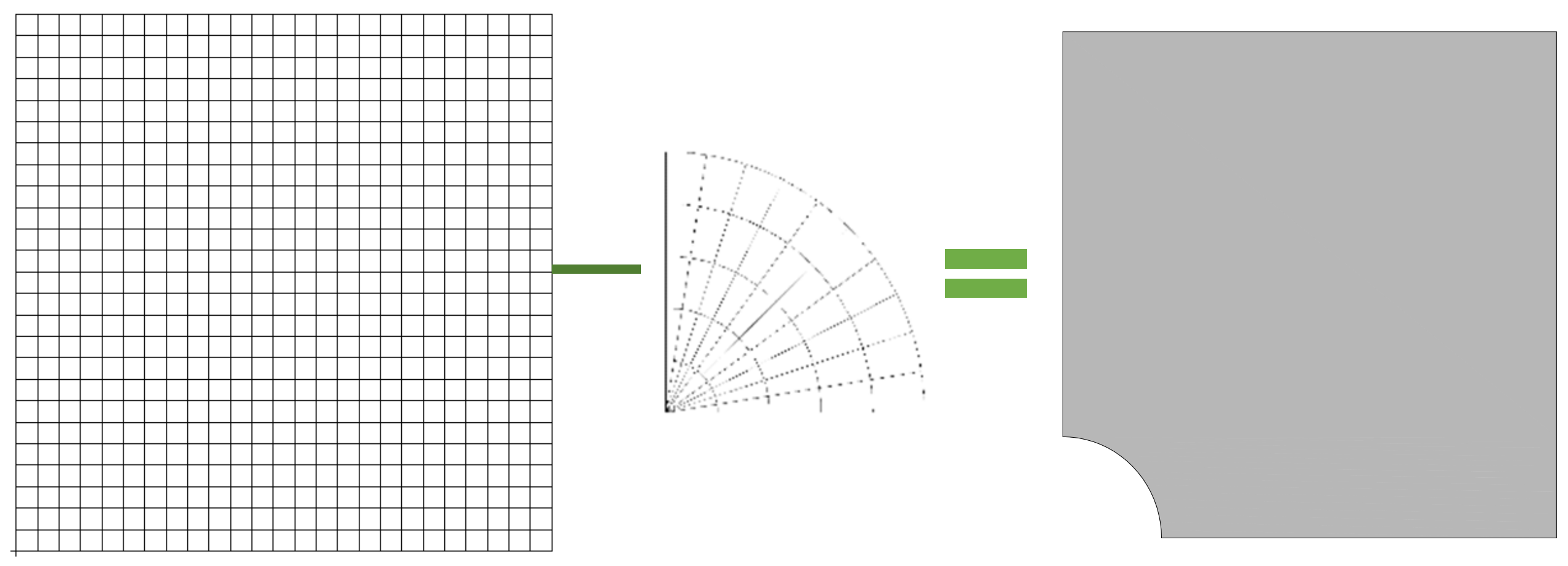
3.2.1. Meshing for a Predesigned Simply Connected Domain

Meshing for an arbitrary simply connected domain is relatively easy. Hybrid triangles are acceptable, while paver triangles with higher quality are still easy to apply, or a more convenient homotopic mesh method can be used, as illustrated in Figure 6.

Homotopic meshing in 2D means the process of mapping the boundary curve $C_1(u)$ to the inner curve $C_2(u)$. Both $C_1(u)$ and $C_2(u)$ are closed NURBS curves, and the arrows in Figure 6c show the circumferential direction of $C_2(u)$. Then, the physical locations of any points $P$ within $C_1(u)$ can be expressed as a function of the circumferential parameter u and radial parameter v by:

$$P=(1-\eta (v))C_1(u)+\eta (v)C_2(u),\hspace{1em}0\le u,v\le 1$$

(19)

If $\eta (v)=v$ and $C_2(u)$ collapses to a point, the homotopic mesh will be the same as the discretization idea in the scaled boundary method. What should be emphasized here is that the curve $C_2(u)$ should be completely within the curve $C_1(u)$. Otherwise, there will be elements (red slashed region in Figure 6d) outside the predesigned domain without field nodes to shape the approximation RPIM basic function. However, a point style $C_2(u)$ does not always exist for a nonconvex domain to ensure that all the elements are located inside the predesigned domain. However, there are still many other ways to accomplish the mesh for an arbitrary simply connected predesigned topology.

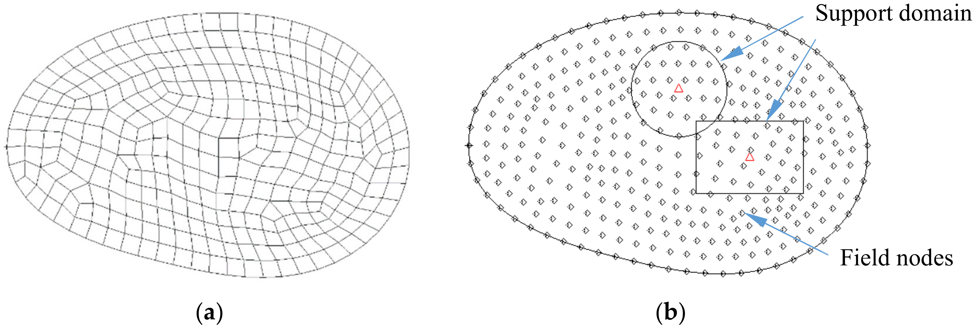
3.2.2. Deploying the Field Nodes

In conventional FEM or meshfree methods, field nodes are only deployed in the material domain within the boundaries. In the proposed method, field nodes are deployed all through the predesigned domain, including the region with holes. This is because the integration of the hole mesh requires the support of field nodes inside the hole.

To deploy the field nodes conveniently, nodes are first settled within a uniform interval in a region larger than the predesigned one. Then, the nodes outside the predesigned domain (blue in Figure 7) are removed using Gauss’ flux theorem, the 2D form of which is

$${\displaystyle \underset{\mathsf{\Gamma }}{\mathsf{\int }}\frac{\stackrel{\rightharpoonup }{R}}{R^2}·d\stackrel{\rightharpoonup }{\Gamma }}=\left\{\begin{array}{cc} 0,& \mathrm{o}\mathrm{u}\mathrm{t}\mathrm{s}\mathrm{i}\mathrm{d}\mathrm{e}\\ 2\pi ,& \mathrm{i}\mathrm{n}\mathrm{s}\mathrm{i}\mathrm{d}\mathrm{e}\end{array}\right.$$

(20)

where R is the Euclidean distance between the field node and the point on the boundary. Zero is just an ideal number to reach in the numerical solution, therefore we define any node with a result less than $\pi$ to be outside. Finally, the remaining nodes are deployed along the boundary of the predesigned domain, as shown in Figure 7, in which purple labels of “12” means the fixed boundary condition in X and Y directions.

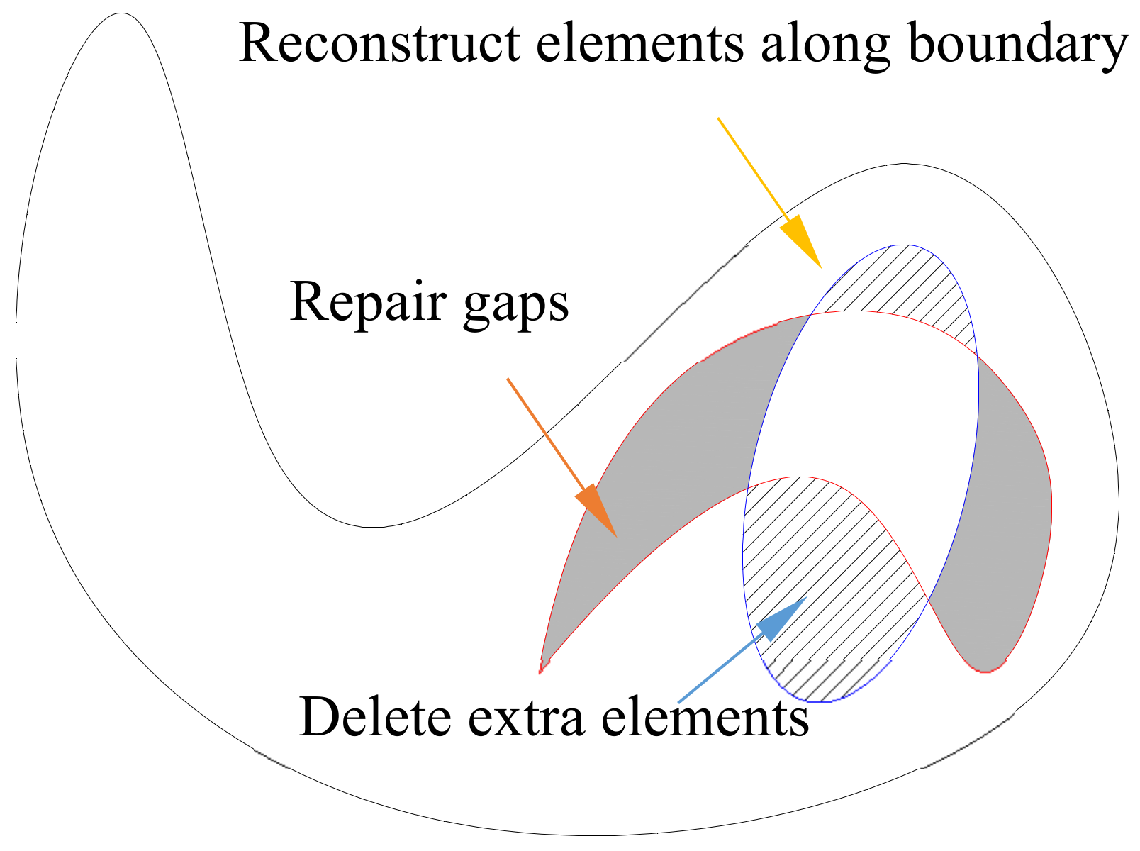
3.2.3. Meshing Homotopically for the Holes

Generally, the point-style homotopic mesh is available for holes of most shapes, unless they are too close to the boundary of the predesigned domain and are nonconvex, which would generate integration meshes outside the predesigned domain. With a point-style homotopic mesh, the integration of a hole can be executed in the parameter domain.

In the point-style homotopic mesh, the hole boundary $C_1(u)$ and reference point $C_2(u)$ are defined as:

$$\begin{array}{l}{C}_1(u)=(x,y)=(f(u),g(u))\\ C_2(u)=(x_0,y_0)\end{array}$$

(21)

Thus, the mapping relationship between physical domain $\mathrm{\Omega }=x\times y$ and parameter domain $\Delta =u\times v$ would be:

$$\left\{\begin{array}{c}x\left(u,v\right)=v\left(f\left(u\right)-x_0\right)+x_0\\ y\left(u,v\right)=v\left(g\left(u\right)-y_0\right)+y_0\end{array}\right.$$

(22)

Then, the hole can be easily meshed in the parameter domain with $n$ numbers in the circumferential direction $u$ and $m$ numbers in the radial direction $v$.

3.2.4. Numerical Integration and Normal Subtraction Technique

The integration on the physical domain for any function $F\left(x,y\right)$ can be transferred to the parameter domain in the form of

$$\begin{array}{ll}{\displaystyle \underset{\mathrm{\Omega }}{\mathsf{\int }\mathsf{\int }}F\left(x,y\right)}dxdy& ={\displaystyle \underset{\Delta }{\mathsf{\int }\mathsf{\int }}F\left[x\left(u,v\right),y\left(u,v\right)\right]}\left|\begin{array}{cc}\frac{\partial x}{\partial u}& \frac{\partial x}{\partial v}\\ \frac{\partial y}{\partial u}& \frac{\partial y}{\partial v}\end{array}\right|dudv\\ \hspace{1em}& ={\displaystyle \underset{\Delta }{\mathsf{\int }\mathsf{\int }}F\left[x\left(u,v\right),y\left(u,v\right)\right]}\cdot v\left[f^{\prime }\left(u\right)g\left(u\right)-f\left(u\right)g^{\prime }\left(u\right)\right]dudv\end{array}$$

(23)

Equation (23) is numerically integrated by standard Gaussian quadrature methods at each element. As the displacement on the Gaussian quadrature point can be expressed by the displacement of local supported field nodes in the RPIM interpolation, the stiffness matrix for a predesigned domain and h holes will be constructed on all the field nodes within the predesigned domain, as illustrated in Figure 7.

In a general 2D linear elastic problem, the stiffness of the jth element in the ith hole can be integrated over the parameter domain $\Delta =u\times v$ by

$$K_j={\displaystyle \sum _{k=1}^{n_g}{w}_k{F}_k\left|J_k\right|}$$

(24)

where $n_g$ is the total number of Gaussian quadrature points in an element, $w_k$ is the Gaussian integral weight of the kth point, and $F_k$ is the stiffness function expressed here as

$$F_k=B_k^{T}D{B}_k$$

(25)

where $B_k$ is the strain matrix and $D$ is the material constant matrix. In addition, $\left|J_k\right|$ in Equation (25) is the area integral Jacobian matrix

$$\left|J_k\right|=v_k\left[f^{\prime }\left(u_k\right)g\left(u_k\right)-f\left(u_k\right)g^{\prime }\left(u_k\right)\right]\frac{{(du)}_j}{2}\frac{{(dv)}_j}{2}$$

(26)

where ${(du)}_j$ and ${(dv)}_j$ are the circumferential and radial lengths, respectively, of the jth element in the parameter domain. As a hole can be easily meshed in the parameter domain with $n$ numbers in the circumferential direction and $m$ numbers in the radial direction, the stiffness matrix of the jth element can be obtained by summing

$$K_i={\displaystyle \sum _{j=1}^{n\times m}{K}_j}$$

(27)

Assuming that the stiffness matrix of the predesigned domain is $K_0$, the total stiffness matrix can be constructed by the integration subtraction technique as follows.

$$(K_0-{\displaystyle \sum _{i=1}^h{K}_i})U=F$$

(28)

Then, the displacement of all the field nodes in Figure 7 is calculated as in the above equation. Even if holes are added or changed, as in Figure 5, no extra field nodes need to be added or deleted.

3.2.5. Moving Subtraction Technique for a Varying Hole

A hole is said to be varying if the control points of the hole are moving and overlapping regions still exist between the new and the old holes. In this case, the moving subtraction technique is more efficient than the normal subtraction technique. However, if no overlapping regions exist, as in faraway translation, implementing the deletion of old holes and the addition of new holes using previous normal subtraction techniques is more practical.

In the moving subtraction technique, when a hole varies from $C_1(u)$ to $C_2(u)$, only the region between $C_1(u)$ and $C_2(u)$ needs to be integrated, as shown in Figure 8. This is mathematically equivalent to the direct operation of deleting hole ${\mathrm{\Omega }}_{C1}$ and adding hole ${\mathrm{\Omega }}_{C2}$ in Equation (29), but with less region to be integrated.

$${\mathrm{\Omega }}_{C2}-{\mathrm{\Omega }}_{C1}={\mathrm{\Omega }}_{(C2-C1)}$$

(29)

As the homotopic mesh is conveniently applied between $C_1(u)$ and $C_2(u)$, as shown with the lines in Figure 8, the new global stiffness matrix can be easily obtained by adding the changing part of $K_{(C2-C1)}$.

4. Numerical Examples

In this section, three linear elasticity examples are presented to investigate the applicability of the proposed integration subtraction technique in a complex domain. The first example of the classic problem of a plate with a circular hole is used to discuss the convergence and efficiency of the presented method. The other two examples of bubbles with two holes are used to verify the feasibility of the complex topology of the normal subtraction technique and the moving subtraction technique.

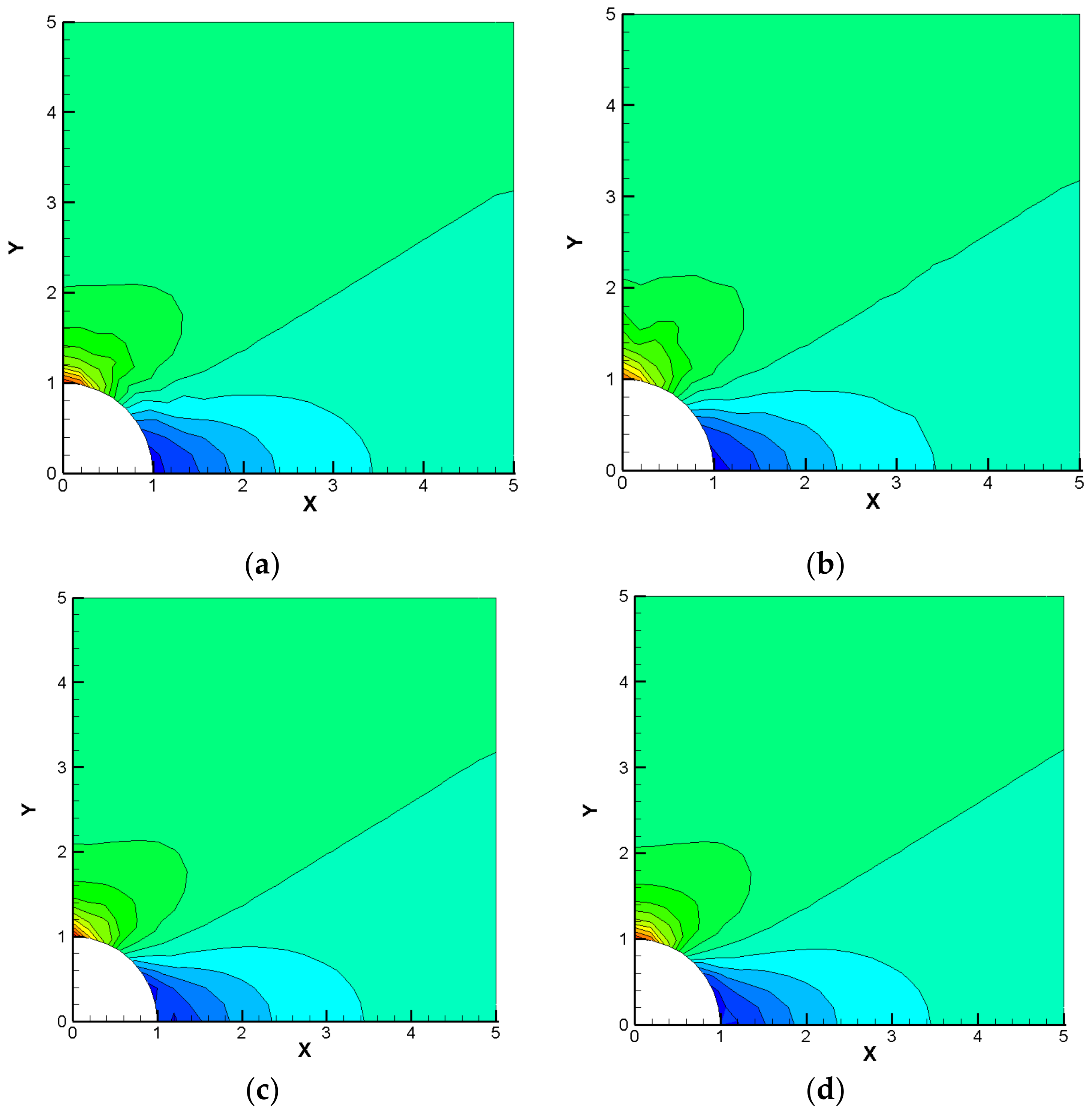
4.1. Infinite Plate with a Circular Hole

The first example is an infinite plate with a circular hole in the center, subjected to a unidirectional tensile load of p = 1.0 in the x-direction, as shown in Figure 9a. Due to symmetry, only one quadrant of the plate is modeled in Figure 9b. The geometry and material properties are as follows: length $L=5$, hole radius $a=1$, Young’s modulus $E={10}^3$, Poisson’s ratio $v=0.3$. The symmetry conditions $u_x=0$ along CD and $u_y=0$ along AB are imposed on the left and bottom edges, respectively. Traction boundary conditions given by the exact solution are imposed on the right (x = 5) and top (y = 5) edges.

The exact stress solution for this problem is:

$${\sigma }_{xx}(x,y)=1-\frac{a^2}{r^2}\left\{\frac{3}{2}\mathrm{c}\mathrm{o}\mathrm{s}2\theta +\mathrm{c}\mathrm{o}\mathrm{s}4\theta \right\}+\frac{3a^4}{2r^4}\mathrm{c}\mathrm{o}\mathrm{s}4\theta$$

(30)

$${\sigma }_{yy}(x,y)=-\frac{a^2}{r^2}\left\{\frac{1}{2}\mathrm{c}\mathrm{o}\mathrm{s}2\theta -\mathrm{c}\mathrm{o}\mathrm{s}4\theta \right\}-\frac{3a^4}{2r^4}\mathrm{c}\mathrm{o}\mathrm{s}4\theta$$

(31)

$${\sigma }_{xy}(x,y)=-\frac{a^2}{r^2}\left\{\frac{1}{2}\mathrm{s}\mathrm{i}\mathrm{n}2\theta +\mathrm{s}\mathrm{i}\mathrm{n}4\theta \right\}+\frac{3a^4}{2r^4}\mathrm{s}\mathrm{i}\mathrm{n}4\theta$$

(32)

On the other hand, a plane stress case is discussed here, for which the exact displacement is:

$$u_x=\frac{p}{4\eta }\left\{\frac{k+1}{2}r\mathrm{c}\mathrm{o}\mathrm{s}\theta +\frac{a^2}{r}\left[\left(1+k\right)\mathrm{c}\mathrm{o}\mathrm{s}\theta +\mathrm{c}\mathrm{o}\mathrm{s}3\theta \right]-\frac{a^4}{r^3}\mathrm{c}\mathrm{o}\mathrm{s}3\theta \right\}$$

(33)

$$u_y=\frac{p}{4\eta }\left\{\frac{k-3}{2}r\mathrm{s}\mathrm{i}\mathrm{n}\theta +\frac{a^2}{r}\left[\left(1-k\right)\mathrm{s}\mathrm{i}\mathrm{n}\theta +\mathrm{s}\mathrm{i}\mathrm{n}3\theta \right]-\frac{a^4}{r^3}\mathrm{s}\mathrm{i}\mathrm{n}3\theta \right\}$$

(34)

where the parameters $\eta$ and $k$ are given by

$$\eta =\frac{E}{2\left(1+v\right)}, k=\frac{3-v}{1+v}$$

(35)

Convergence and efficiency are first compared in the three tested methods, which are the presented integration subtraction method, the traditional RPIM meshfree method, and the bilinear isoparametric FEM, denoted hereafter as RSUB, RPIM and FEM, respectively. In the traditional meshfree RPIM, the mesh is the same as in the FEM, in which the nodes and elements are treated as field nodes and background cells, respectively.

The discretization of RSUB using integration meshes and the subtraction process is shown in Figure 10, while the discretization of RPIM and FEM is shown in Figure 11. A node interval of $h=0.2$ is used for illustration.

The errors in displacement and energy are evaluated by

$$E^{disp}=\sqrt{\frac{{\displaystyle {\sum }_{I=1}^n{(u_I^q-u_I^e)}^T(u_I^q-u_I^e)}}{{\displaystyle {\sum }_{I=1}^n{\left(u_I^e\right)}^T{u}_I^e}}}$$

(36)

$$E^{neg}=\sqrt{\frac{{\displaystyle \underset{\Omega }{\int }{({\epsilon }^h-{\epsilon }^e)}^{T}D({\epsilon }^h-{\epsilon }^e)}}{{\displaystyle \underset{\Omega }{\int }{({\epsilon }^e)}^{T}D{\epsilon }^e}}}$$

(37)

where the superscript e denotes the exact solutions, while the superscript q denotes the numerical solutions. The five different node intervals h = 0.25, 0.2, 0.125, 0.1, and 0.0625 are investigated.

In Figure 12, the two meshfree methods, RPIM and RSUB, demonstrate higher accuracy than FEM in displacement and energy, with RSUB appearing to be the most accurate among the three tested methods. The better accuracy of RSUB with coarse mesh may be obtained by the duplicate integration for subtraction, which may be able to improve the result around the boundary of hole. When the node interval gets smaller, this advantage in precision of RSUB becomes less significant and converges to RPIM. In addition to having greater displacement accuracy, RPIM has higher convergence rates. Moreover, the presented RSUB method achieves extremely high accuracy on a rough mesh. However, with respect to energy, the convergence processes of RPIM and RSUB are not good, although their accuracy is better than that of FEM. It has been shown by Liu and Gu [40] that a purely MQ-RBF cannot always ensure to exactly reproduce a linear field function. This could be one of the major reasons for the poor h-convergence in using MQ-RBF for field variable interpolations.

As a result of the shortcomings of the MQ-RBF, its energy efficiency is still not satisfactory. However, with regard to displacement, the meshfree methods, RPIM and RSUB, achieve better efficiency than FEM, as shown in Figure 13. While RSUB seems to be a little more time consuming than RPIM, the duplicate integration in the hole region for subtraction yields greater accuracy. Thus, RSUB is actually more efficient than RPIM.

Figure 14 shows the ${\sigma }_{xx}$ distribution of this example, recovered in the same method that was illustrated in the mesh with node interval $h=0.2$. Obvious oscillations can be observed in the results of FEM and RPIM. In contrast, the proposed RSUB method results in a smooth stress field and no spurious oscillations present. This is compatible with the previous super accuracy property of RSUB.

4.2. Bubble with Arbitrary Holes

As the problem of a single circular hole dug in the predesigned domain of a rectangle has been verified above, we now propose another example of an arbitrary domain: a bubble with arbitrary holes. In FEM, this bubble is discretized with an edge length of 0.03 with paver quad4 meshes, as illustrated in Figure 15. The material properties and constraints are as follows: Young’s modulus $E={10}^3$, Poisson’s ratio $v=0.3$, the left and right side of the bubble are fixed in X and Y directions (shown with purple labels “12” in Figure 15), and a single force of 1.0 is applied to the upper side. As for the presented method, the predesigned domain and holes are all discretized in a point-style homotopic mesh, with $n$ numbers in the circumferential direction and $m$ numbers in the radial direction, as marked in Figure 16. Field nodes are deployed at a uniform interval of 0.04 within the predesigned domain with the same nodes as FEM along the boundary, as shown in Figure 16c.

In the presented RSUB method, the displacement and stress of the example are solved in the stiffness matrix constructed on the field nodes, as in Figure 16c. Then, the displacement and stress in the y-direction are compared for FEM, RPIM and RSUB, as shown in Figure 17. In addition, the detailed results of the displacement of nodes on the upper side of the boundary are listed in Figure 18 at the cusp where the force is loaded.

Comparing the solutions of displacement and stress in Figure 17 and Figure 18, it is obvious that the RSUB results are consistent with those of RPIM and FEM. However, little oscillation is found near the boundary of the right-side irregular hole in the stress results of RSUB. The reason would be that the difference between the displacement of field nodes inner and outer the hole is too great. While in the stress recovery process, both of inner and outer field nodes are needed. In addition, stress is only accurately solved at the Gaussian interpolation point, so oscillation may appear in the recovery result on the boundary of hole.

4.3. Bubble with Varied Holes

The bubble with varied holes is considered here to verify the feasibility of the moving integration subtraction technique. Unlike the previous bubble, the hole with a complex boundary on the right side is changed from a red hole to a blue one in Figure 19b. Nevertheless, the essential boundary and natural boundary with a single traction force remain the same. There is no need to adjust the field nodes. The discretization in FEM and the mesh between varied holes (shown with a shadow line) are illustrated in Figure 19, in which purple labels of “12” means the fixed boundary condition in X and Y directions.

The moving subtraction technique, which has been discussed in Section 3.2.5, is called RMOV for brevity. The shadow line in Figure 19b shows the discretization in the circumferential direction. The material property and constraints, the parameters of the point-style homotopic meshes of the circle hole, and the outer boundary remain unchanged. Then, the results of displacement and stress in the y-direction are compared among the four methods of FEM, RPIM, RSUB, and RMOV in Figure 20. The detailed displacement in the y-direction near the force is plotted in Figure 21.

Comparing the solution of displacement and stress given by the four methods in Figure 20 and Figure 21, it can be seen that the result of RMOV is consistent with those of the other three methods. Therefore, RMOV is more efficient in dealing with hole-varying problems than RSUB, as RMOV requires less integration than RSUB. On the other hand, RMOV causes less oscillation than RSUB near a hole boundary with a complex shape in the stress field. Therefore, RMOV is more suitable for addressing hole-varying problems.

5. Conclusions

A NURBS-enhanced meshfree method with an integration subtraction technique is developed to model holes interactively in a predesigned domain for adaptive problems. With this method, the integration domain with complex topology can be easily and exactly described by its boundaries. By combining this method with the homotopic mesh method, any holes can be directly dug out from the predesigned domain with no refinement. In addition, a more efficient moving subtraction method is expanded to speed up hole-varying problems, in which only the region between the new and old holes boundaries must be integrated. The major discoveries arising from the comparison among FEM, RPIM, RSUB, and RMOV are as follows:

1.

Both RPIM and RSUB are more accurate than FEM and show higher convergence in displacement but do not have good enough energy convergence.

2.

The proposed RSUB method achieves superior accuracy on a coarse mesh and a smoother stress result with a regular hole.

3.

The duplicated integration of holes for subtraction yields improvements in precision, making RSUB more efficient than the original RPIM.

4.

The results of both the proposed RSUB method and RMOV in displacement and stress are in good agreement with those of FEM and RPIM but cause little oscillation in the stress field near the boundary of the irregular hole, with RMOV causing less than RSUB.

In conclusion, the proposed integration subtraction technique not only provides a convenient mesh for complex topology but also demonstrates excellent accuracy and good efficiency. Unfortunately, its performance in energy convergence is not good, and little oscillation around an irregular hole appears in the method. Other integration methods, such as nodal integration, may improve the performance in the area of energy convergence and greatly decrease the computation cost. Moreover, a new stress recovery method can be developed to eliminate the oscillation. These are the two major aspects of planned future work to perfect the proposed method.

References

1. Nguyen, V.P.; Anitescu, C.; Bordas, S.P.A.; Rabczuk, T. Isogeometric analysis: An overview and computer implementation aspects. Math. Comput. Simul. 2015, 117, 89–116. [Google Scholar] [CrossRef] [Green Version]
2. Hughes, T.J.R.; Cottrell, J.A.; Bazilevs, Y. Isogeometric analysis: CAD, finite elements, NURBS, exact geometry and mesh refinement. Comput. Methods Appl. Mech. Eng. 2005, 194, 4135–4195. [Google Scholar] [CrossRef] [Green Version]
3. Cottrell, J.A.; Hughes, T.J.R.; Reali, A. Studies of refinement and continuity in isogeometric structural analysis. Comput. Methods Appl. Mech. Eng. 2007, 196, 4160–4183. [Google Scholar] [CrossRef]
4. Bazilevs, Y.; Calo, V.M.; Cottrell, J.A.; Hughes, T.J.R.; Reali, A.; Scovazzi, G. Variational multiscale residual-based turbulence modeling for large eddy simulation of incompressible flows. Comput. Methods Appl. Mech. Eng. 2007, 197, 173–201. [Google Scholar] [CrossRef]
5. Bazilevs, Y.; Calo, V.M.; Zhang, Y.; Hughes, T.J.R. Isogeometric fluid–structure interaction analysis with applications to arterial blood flow. Comput. Mech. 2006, 38, 310–322. [Google Scholar] [CrossRef]
6. Lipton, S.; Evans, J.A.; Bazilevs, Y.; Elguedj, T.; Hughes, T.J.R. Robustness of isogeometric structural discretizations under severe mesh distortion. Comput. Methods Appl. Mech. Eng. 2010, 199, 357–373. [Google Scholar] [CrossRef]
7. Hughes, T.J.R.; Reali, A.; Sangalli, G. Efficient quadrature for NURBS-based isogeometric analysis. Comput. Methods Appl. Mech. Eng. 2010, 199, 301–313. [Google Scholar] [CrossRef]
8. Kim, H.-J.; Seo, Y.-D.; Youn, S.-K. Isogeometric analysis with trimming technique for problems of arbitrary complex topology. Comput. Methods Appl. Mech. Eng. 2010, 199, 2796–2812. [Google Scholar] [CrossRef]
9. Kim, H.-J.; Seo, Y.-D.; Youn, S.-K. Isogeometric analysis for trimmed CAD surfaces. Comput. Methods Appl. Mech. Eng. 2009, 198, 2982–2995. [Google Scholar] [CrossRef]
10. Xu, J.; Chen, F.; Deng, J. Two-dimensional domain decomposition based on skeleton computation for parameterization and isogeometric analysis. Comput. Methods Appl. Mech. Eng. 2015, 284, 541–555. [Google Scholar] [CrossRef]
11. Xu, G.; Li, M.; Mourrain, B.; Rabczuk, T.; Xua, J.; Bordas, S.P.A. Constructing IGA-suitable planar parameterization from complex CAD boundary by domain partition and global/local optimization. Comput. Methods Appl. Mech. Eng. 2018, 328, 175–200. [Google Scholar] [CrossRef] [Green Version]
12. Hamrani, A.; Habib, S.H.; Belaidi, I. CS-IGA: A new cell-based smoothed isogeometric analysis for 2D computational mechanics problems. Comput. Methods Appl. Mech. Eng. 2017, 315, 671–690. [Google Scholar] [CrossRef]
13. Sevilla, R.; Fernández-Méndez, S.; Huerta, A. NURBS-enhanced finite flement method (NEFEM). Arch. Comput. Methods Eng. 2008, 76, 56–83. [Google Scholar] [CrossRef] [Green Version]
14. Bazilevs, Y.; Calo, V.M.; Cottrell, J.A.; Evans, J.A.; Hughes, T.J.R.; Lipton, S.; Scott, M.A.; Sederberg, T.W. Isogeometric analysis using T-splines. Comput. Methods Appl. Mech. Eng. 2010, 199, 229–263. [Google Scholar] [CrossRef] [Green Version]
15. Dörfel, M.R.; Jüttler, B.; Simeon, B. Adaptive isogeometric analysis by local h-refinement with T-splines. Comput. Methods Appl. Mech. Eng. 2010, 199, 264–275. [Google Scholar] [CrossRef] [Green Version]
16. Javier, V.; Felipe, C.; Hoang, X.; Nguyen, E.A. Application of PHT-splines in bending and vibration analysis of cracked Kirchhoff–Love plates. Comput. Methods Appl. Mech. Eng. 2020, 361, 112754. [Google Scholar] [CrossRef]
17. Valizadeh, N.; Bazilevs, Y.; Chen, J.S.; Rabczuk, T. A coupled IGA–meshfree discretization of arbitrary order of accuracy and without global geometry parameterization. Comput. Methods Appl. Mech. Eng. 2015, 293, 20–37. [Google Scholar] [CrossRef]
18. Thai, C.H.; Nguyen, T.N.; Rabczuk, T.; Nguyen-Xuan, H. An improved moving kriging meshfree method for plate analysis using a refined plate theory. Comput Struct. 2016, 176, 34–49. [Google Scholar] [CrossRef]
19. Greco, F.; Coox, L.; Maurin, F.; Desmet, W. NURBS-enhanced maximum-entropy schemes. Comput. Methods Appl. Mech. Eng. 2017, 317, 580–597. [Google Scholar] [CrossRef]
20. Zhang, H.; Wang, D. An isogeometric enriched quasi-convex meshfree formulation with application to material interface modeling. Eng. Anal. Bound. Elem. 2015, 60, 37–50. [Google Scholar] [CrossRef]
21. Gingold, R.A.; Monaghan, J.J. Smoothed Particle Hydrodynamics—Theory and Application to Non-Spherical Stars. Mon. Not. R. Astron. Soc. 1977, 181, 375–389. [Google Scholar] [CrossRef]
22. Lucy, L.B. A numerical approach to the testing of the fission hypothesis. Astron. J. 1977, 82, 1013–1024. [Google Scholar] [CrossRef]
23. Liu, M.B.L.G.R. Smoothed Particle Hydrodyndmics a Mesh Free Particle Method; World Scientific Publishing Co., Pte. Ltd.: Singapore, 2003. [Google Scholar]
24. Belytschko, T.; Lu, Y.Y.; Gu, L. Element-free Galerkin methods. Int. J. Numer. Meth. Eng. 1994, 37, 229–256. [Google Scholar] [CrossRef]
25. Kansa, E.J. Multiquadrics—A scattered data approximation scheme with applications to computational fluid-dynamics-I surface approximations and partial derivative estimates. Comput. Math. Appl. 1990, 19, 127–145. [Google Scholar] [CrossRef] [Green Version]
26. Liu, G.R. Meshfree Methods: Moving Beyond the Finite Element Method; CRC Press: Boca Raton, FL, USA, 2010. [Google Scholar]
27. Simpson, R.N.; Bordas, S.P.A.; Trevelyan, J.; Rabczuk, T. A two-dimensional isogeometric boundary element method for elastostatic analysis. Comput. Methods Appl. Mech. Eng. 2012, 209–212, 87–100. [Google Scholar] [CrossRef]
28. Natarajana, S.; Wang, J.; Song, C.; Birk, C. Isogeometric analysis enhanced by the scaled boundary finite element method. Comput. Struct. 2015, 283, 733–762. [Google Scholar] [CrossRef]
29. Katsikadelis, J.T. Boundary Elements: Theory and Applications; Elsevier: Amsterdam, The Netherlands, 2002. [Google Scholar]
30. Song, C.; Wolf, J.P. The scaled boundary finite-element method—Alias consistent infinitesimal finite-element cell method—For elastodynamics. Comput. Methods Appl. Mech. Eng. 1997, 147, 329–355. [Google Scholar] [CrossRef]
31. Liu, J.; Li, J.; Li, P.; Lin, G.; Xu, T.; Chen, L. New application of the isogeometric boundary representations methodology with SBFEM to seepage problems in complex domains. Comput. Fluids 2018, 174, 241–255. [Google Scholar] [CrossRef]
32. Chasapi, M.; Klinkel, S. A scaled boundary isogeometric formulation for the elasto-plastic analysis of solids in boundary representation. Comput. Methods Appl. Mech. Eng. 2018, 333, 475–496. [Google Scholar] [CrossRef]
33. Gu, J.; Zhang, J.; Li, G. Isogeometric analysis in BIE for 3-D potential problem. Eng. Anal. Bound. Elem. 2012, 36, 858–865. [Google Scholar] [CrossRef]
34. Heltai, L.; Arroyo, M.; DeSimone, A. Nonsingular isogeometric boundary element method for Stokes flows in 3D. Comput. Methods Appl. Mech. Eng. 2014, 268, 514–539. [Google Scholar] [CrossRef] [Green Version]
35. Heltai, L.; Arroyo, M.; DeSimone, A. A review of the scaled boundary finite element method for two-dimensional linear elastic fracture mechanics. Eng. Fract. Mech. 2018, 187, 45–73. [Google Scholar] [CrossRef] [Green Version]
36. Farin, G.; Hoschek, J.; Kim, M.-S. Handbook of Computer Aided Geometric Design; Elsevier: Amsterdam, The Netherlands, 2002. [Google Scholar]
37. Piegl, L.; Tiller, W. The NURBS Book; Springer: Berlin/Heidelberg, Germany, 1997. [Google Scholar]
38. Chen, J.-S.; Hillman, M.; Chi, S.-W. Meshfree methods: Progress made after 20 Years. J. Eng. Mech. 2007, 143, 04017001. [Google Scholar] [CrossRef] [Green Version]
39. Golberg, M.A.; Chen, C.S.; Bowman, H. Some recent results and proposals for the use of radial basis functions in the BEM. Eng. Anal. Bound. Elem. 1999, 23, 285–296. [Google Scholar] [CrossRef]
40. Liu, G.R.; Gu, Y.T. A meshfree method: Meshfree weak–strong (MWS) form method for 2-D solids. Comput. Mech. 2003, 33, 2–14. [Google Scholar] [CrossRef]
Figure 1. Integration subtraction technique (a) − (b) = (c): (a) a predesigned integration domain with isogeometric triangular meshes (along the blue boundary) and finite element (FE) triangular meshes; (b) different holes integration domains with homotopic meshes to be subtracted; (c) equivalent material domains for different holes.
Applsci 10 02587 g001
Figure 2. Example of a B-spline basic function and control points (black solid dots).
Applsci 10 02587 g002
Figure 3. (a) Finite element method (FEM) with a local element; (b) meshfree approximation function constructed by field nodes within a support domain.
Applsci 10 02587 g003
Figure 4. (a) Hybrid triangle meshes; (b) Gaussian quadrature points in boundary and inner elements.
Applsci 10 02587 g004
Figure 5. Measurement for refinement in the traditional method when the hole is changed.
Applsci 10 02587 g005
Figure 6. (a) Hybrid triangle mesh; (b) paver triangle mesh; (c) homotopic mesh; (d) homotopic mesh in point style.
Applsci 10 02587 g006
Figure 7. Removed nodes (blue) and field nodes (red) in a predesigned domain with a hole.
Applsci 10 02587 g007
Figure 8. Moving subtraction when a hole varies from C1 (red) to C2 (blue).
Applsci 10 02587 g008
Figure 9. Infinite plate with a circular hole: (a) problem description; (b) quadrant numerical model.
Applsci 10 02587 g009
Figure 10. Discretization of RSUB with node interval h = 0.2.
Applsci 10 02587 g010
Figure 11. Discretization of FEM and radial point interpolation method (RPIM) with node interval h = 0.2.
Applsci 10 02587 g011
Figure 12. Convergence in the problem of the plate with a hole: (a) displacement; (b) energy.
Applsci 10 02587 g012
Figure 13. Computational efficiency in the problem of the plate with a hole: (a) displacement; (b) energy.
Applsci 10 02587 g013
Figure 14. Stress fields in the problem of the plate with a hole obtained by (a) FEM; (b) RPIM; (c) RSUB; (d) exact solution.
Applsci 10 02587 g014
Figure 15. Discretization and constraints in FEM.
Applsci 10 02587 g015
Figure 16. Discretization of RSUB in a point-style homotopic mesh: (a) predesigned domain, (b) arbitrary holes, (c) deployment of field nodes, (d) actual equivalent problem.
Applsci 10 02587 g016
Figure 17. Displacement in y-direction of different methods: (a) FEM; (c) RPIM; (e) RSUB. Stress in y-direction of different methods: (b) FEM; (d) RPIM; (f) RSUB.
Applsci 10 02587 g017
Figure 18. Displacement in the y-direction along the upper side of the boundary.
Applsci 10 02587 g018
Figure 19. (a) Discretization and constraints in FEM of varied bubbles, (b) mesh between varied boundaries.
Applsci 10 02587 g019
Figure 20. Displacement in y-direction of different methods: (a) FEM; (c) RPIM; (e) RSUB; (g) RMOV. Stress in y-direction of different methods: (b) FEM; (d) RPIM; (f) RSUB; (h) RMOV
Applsci 10 02587 g020
Figure 21. Displacement in the y-direction along the upper side of the boundary.
Applsci 10 02587 g021