Advanced Parameter-Setting-Free Harmony Search Algorithm

Abstract

In this paper, we propose an advanced parameter-setting-free (PSF) scheme to solve the problem of setting the parameters for the harmony search (HS) algorithm. The use of the advanced PSF method solves the problems of the conventional PSF scheme that results from a large number of iterations and shows good results compared to fixing the parameters required for the HS algorithm. In addition, unlike the conventional PSF method, the advanced PSF method does not use additional memory. We expect the advanced PSF method to be applicable to various fields that use the HS algorithm because it reduces the memory utilization for operations while obtaining better results than conventional PSF schemes.

1. Introduction

A metaheuristic is a heuristic technique that can be applied to various problems irrespective of the type and information of the problem. Various such methods have been proposed, including the representative genetic algorithm. This metaheuristic method is a technique that can be optimized not only in engineering but also in various other fields, such as natural science, business administration, and social science, because of the simplicity of its concept and theory.

The harmony search (HS) algorithm [1] is one of the metaheuristic algorithms and was inspired by the musical idea of finding each instrument’s notes by modifying each one a little bit, to create harmony among the instrument’s notes. Similarly, the HS algorithm has the characteristic that the variable data that gives the best result in the memory called harmony memory (HM) can be stored and updated during the execution of the algorithm, and the value stored in the HM can be used for the next iteration. The HS algorithm has been used in various fields because it is easy to apply in any field and has the advantage of fast convergence and proper results [2,3].

It is common to use random values for each variable when performing HS but to use the values in HM as they are or change them slightly depending on the probability. The performance of the HS algorithm depends on the parameters that determine this probability. When the HS algorithm is used, the parameters of the harmony memory consideration rate (HMCR) and pitch adjustment rate (PAR) are determined according to the type of problem and the number of variables required for the problem. It is important. In general, these two parameters are set manually by a human and fixed during HS operation, but this does not apply to the change of HM according to the progress of the operation. Therefore, many executions are needed overall. To solve this problem, a parameter-setting-free (PSF) method [4,5,6] has been proposed. In this method, if the result is stored in HM, the variables used to derive the value are stored separately, and the result is put in HM to determine the value of HMCR and PAR for each variable. However, this method can make the value of HMCR and PAR 0 or 1 before the maximum iterations are reached. If the value of HMCR or PAR becomes 0 or 1, even if HS is performed, it is difficult to produce good results because new random values are not used in certain variables or only some variables are changed.

Jiang et al. [7] proposed a method that modifies the values of HMCR and PAR with predefined values near 0 or 1 when they result in 1 or 0 during the execution of HS. However, the problem with such a method is that the values of HMCR and PAR are fixed at the predefined values after a certain number of iterations. We propose a novel PSF scheme that the HMCR and PAR values are automatically adjusted to converge into a certain value in the range of 1 and 0 following the optimization problem during the optimization process of HS.

In this paper, we explain and interpret the meaning of the HMCR and PAR values in the HS algorithm and present an advanced PSF scheme for these parameters. Section 2 will look at the basic parameters of the HS algorithm and how the HS algorithm works, and it describes the conventional PSF scheme and the problems that occur when using it. Section 3 proposes our advanced PSF scheme and explains why it is good to use the advanced PSF scheme. Section 4 compares the results between the HS algorithm using fixed HMCR and PAR, the existing PSF HS algorithm, and the new PSF HS algorithm.

2. Conventional HS Algorithm

2.1. Basic HS Algorithm

The HS algorithm, one of the metaheuristic algorithms, is analogous to finding harmony in music. In music, to match the harmony of the notes made by various instruments, the existing good harmony is memorized, and each instrument is tuned slightly in the harmony. The HS algorithm stores the best value of the existing operation values in the HM and applies it by stochastic extraction or by slightly modifying it. Through this, tuning to the best value is the defining characteristic of the HS algorithm.

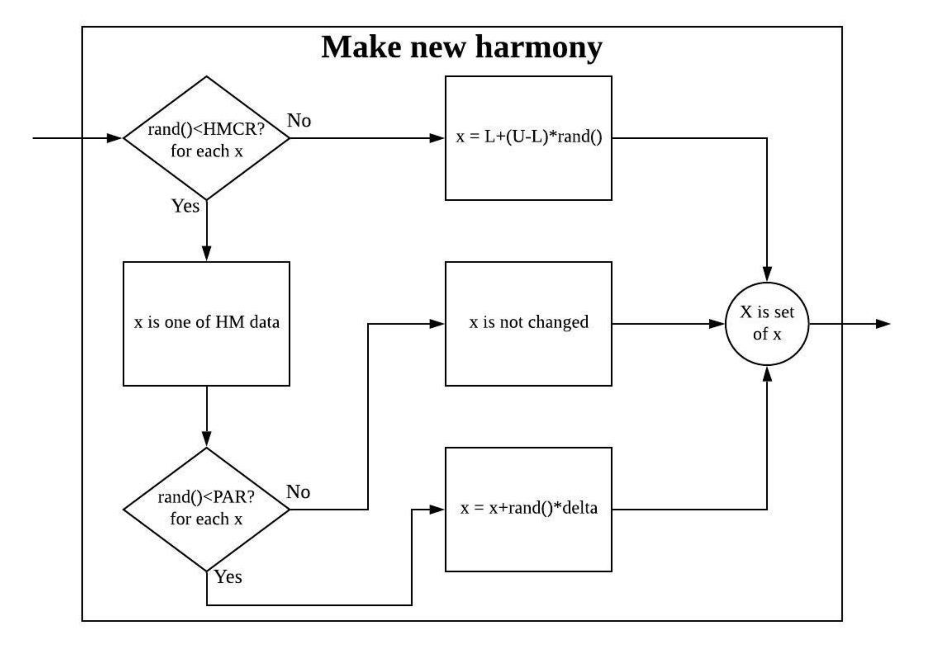
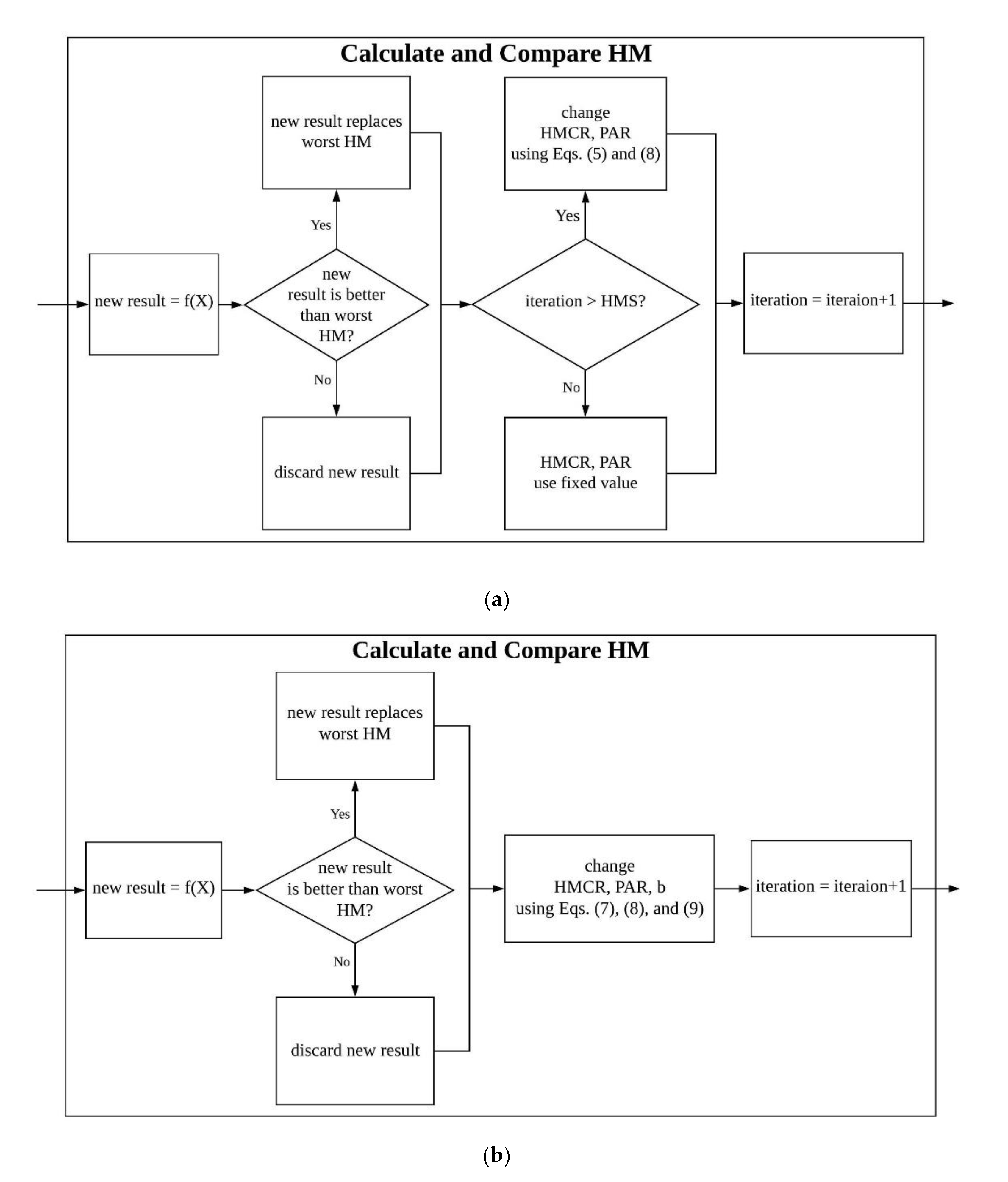
The basic flow of HS is shown in Figure 1, and the main parameters of the HS algorithm are as follows:

• HMCR: the probability of using one of the values in the existing HM when performing HS;
• PAR: the probability of slight variation when using existing HM values with HMCR;
• Pitch adjusting bandwidth (${\mathrm{b}}_{\mathrm{w}}$: the maximum amount of change with PAR;
• Harmony memory size (HMS): the size of HM (number of harmonies stored in HM).

When performing HS, the maximum improvisation (MI), which is the object value or the maximum number of iterations, is used to perform calculations until attaining this specified value or the maximum iterations. This parameter is used as a condition to stop the HS algorithm. Therefore, maximum improvisations are one of the parameters that must be determined by a person, according to the problem to be performed, when using HS.

2.2. Conventional Parameter-Setting-Free HS

HMCR and PAR, which are parameters used in HS, are important parameters that affect the performance of the HS algorithm because they determine whether to use the variable in HM that stores the best value among previously calculated values or to change and use it. It is shown in Figure 2. In general HS algorithm, HMCR and PAR are explicitly set to fixed values. Many reports on adaptive HS [8,9,10,11,12,13], which are used to determine HMCR and PAR, have been published, but these only provide the basic values; however, the PSF HS algorithm is proposed for automatically determining such HMCR and PAR.

The conventional PSF HS algorithm [4] first performs a fixed number of iterations with a fixed HMCR and PAR and then stores information about whether the values stored in HM are random values, existing values (HMCR), or changes to existing values (PAR) in each new memory. Figure 3 shows the change of HMCR and PAR when the periodic function, one of the test functions, is executed with the conventional PSF scheme with four variables. As shown in Equations (1) and (2), the number of times the values stored in HM are divided by HMS is used as the HMCR and PAR.

$${\mathrm{HMCR}}_i=\frac{n\left(y_i^j=Memory\right)}{\mathrm{HMS}}$$

(1)

$${\mathrm{PAR}}_i=\frac{n\left(y_i^j=Pitch\right)}{\mathrm{HMS}}$$

(2)

The conventional PSF HS has the advantage of changing the HMCR and PAR by determining the current implementation method according to the existing performance. However, as the number of repetitions increases, the HMCR and PAR values of each variable become 1 or 0. After a certain number of repetitions, certain variables use only combinations or random values as the values of HM, and only specific variables are adjusted. This makes it hard to get better results. It also has the disadvantage of requiring additional memory to store the work done for each HM variable.

PSF HS has the advantage that even when using a variable value for setting HMCR and PAR, the value may be specified without a parameter, unlike other methods where there is at least one part that needs to be determined by the user. However, there is a problem that HMCR and PAR converge to 0 or 1 after a certain number of HS iterations. Due to this problem, some papers [6,14] using PSF HS have proposed modifying HMCR and PAR as in Equations (3) and (4).

$${\mathrm{HMCR}}_i=\min (\frac{n\left(y_i^j=Memory\right)}{\mathrm{HMS}}, HMC{R}_{min})$$

(3)

$${\mathrm{PAR}}_i=\max (\frac{n\left(y_i^j=Pitch\right)}{\mathrm{HMS}},PA{R}_{max})$$

(4)

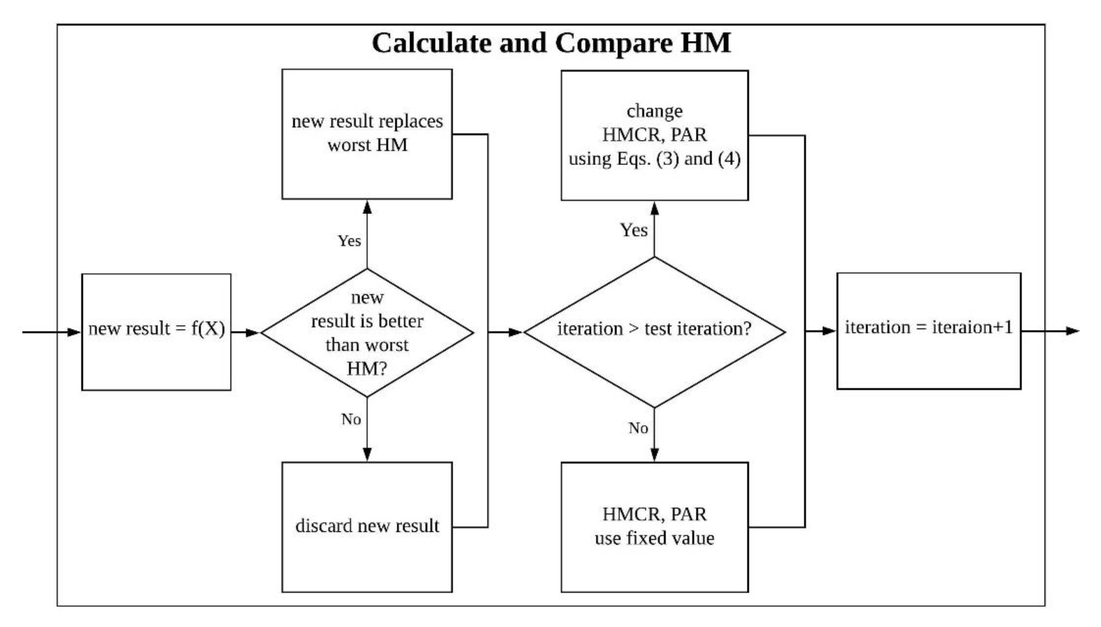
This approach ensures that the HMCR and PAR do not converge to zero or one. $HMC{R}_{min}$ is set to a value near 1, and $PA{R}_{max}$ is set to a value near 0. All conventional PSF schemes in this study use the results calculated with $HMC{R}_{min}=0.99$ and $PA{R}_{max}=0.01$. Applying conventional PSF to HS is equivalent to changing the “Calculate and Compare HM” box in Figure 1, Figure 2, Figure 3 and Figure 4.

3. Advanced Parameter-Setting-Free HS

A PSF scheme has the advantage of not requiring the parameters of the HS algorithm to be set. However, in the case of the conventional PSF method, there is a disadvantage that only one value is used after some progress of the HS. Therefore, to solve this problem, we propose an advanced PSF scheme that uses a maximum improvisation setting to perform HS while considering the HMCR and PAR.

The smaller the HMCR value, the higher the probability that a new random value will be used, and thus the lower the probability of falling into a local solution, but the lower the convergence probability. The higher the HMCR value, the higher is the probability that the value stored in the HM will be used; hence, the probability of convergence increases, but the probability of falling into a local solution also increases. Even if the value of HMCR is the same, as the number of variables increases, the probability of convergence decreases. Therefore, the greater the number of variables, the higher is the HMCR value used. For this reason, the following HMCR adjustments are necessary to improve the results using HS. Early in the iteration of HS, low HMCR values are used to obtain various solutions. As the HS is repeated, the value of HM is used to increase the HMCR value so that the stored value can be finely adjusted. Additionally, the larger the number of variables, the higher should be the HMCR value from the beginning.

As to using the value stored in the HM, the smaller the PAR value, the higher the probability of using the value stored in the HM. Conversely, when using values stored in HM, the higher the PAR value, the more likely it is to change the value to be used slightly, so the probability of adjusting the value increases. In the event of many variables, even a low PAR value can change many of these values by small amounts. Therefore, the higher the HMCR, the higher is the probability of using the value stored in HM and the easier it is to adjust the overall value if the PAR is further adjusted. Moreover, the more variables that are adjusted in HS, the lower the PAR value is, so that many of the variables cannot be changed at once.

In this study, the novel PSF scheme was proposed considering the above conditions. The following sections described the advanced PSF HS algorithm in detail.

3.1. HMCR Dependent on Iteration

The HMCR needs to gradually increase as HS repeats to reach the desired object value. However, in many cases it is not possible to set an object value. Further, the maximum iteration is MI, which must be used if an object value is not specified. Therefore, in these conditions, iteration should be used to determine the HMCR value. The equation for this is:

$$\mathrm{HMCR}=0.5+0.5\times sigmoid\left(10\frac{i}{n}-\frac{5}{\log \left(n\left(val\right)\right)}\right)$$

(5)

In Equation (5) that uses the maximum iterations, $i$ is current iterations; n is maximum iterations, and $n\left(val\right)$ is the number of variables to be changed to HS.

The sigmoid function is:

$$sigmoid\left(x\right)=\frac{1}{1+e^{-x}}$$

(6)

The sigmoid function in Equation (6) has a value of 0.5 for $sigmoid\left(0\right)$. A negative input value produces an output close to zero, and a positive input value produces an output close to one.

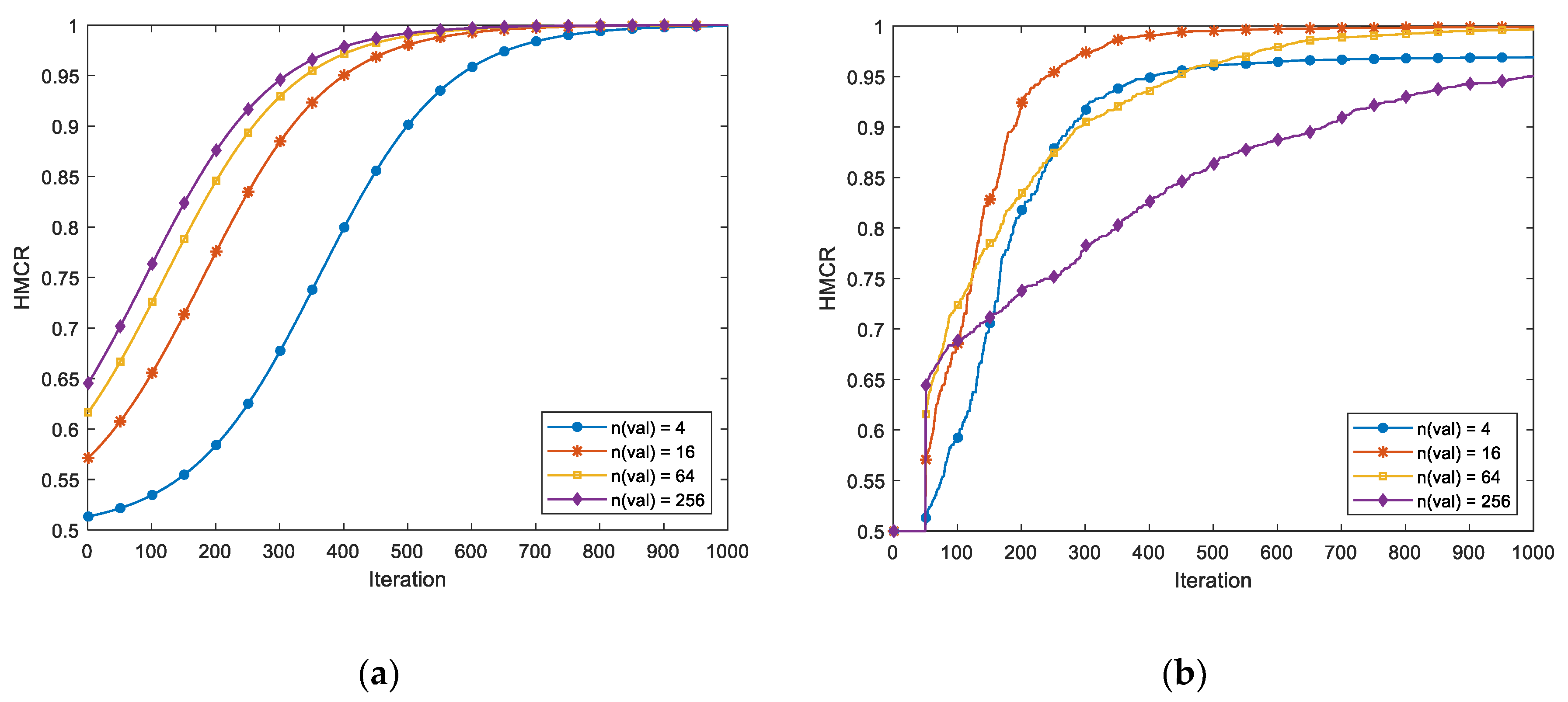
By applying the sigmoid function to the HMCR, it is possible to have a value within the range of 0.5 to 1. This results in a lower HMCR at the beginning of the operation and a higher HMCR value as the performance progresses. This takes the form of Figure 5a. As the HS progresses, the probability of using the value in the existing HM increases, so that the existing value is used rather than the new value, and fine adjustment is possible through the probability of the PAR. In addition, the logarithm of the number of variables is used so that for a larger number of variables, the overall function moves more to the left. This is because, when several variables are changed to new values at once, it is difficult to achieve results as good as those by simply using random values. Therefore, the more the variables, the larger must be the HMCR value.

3.2. HMCR Dependent on Object

As the result of HS approaches the target value, it is necessary to increase the value of HMCR. Additionally, the object value is MI, which must be used unless the maximum iteration was specified. Even when using the maximum iteration, the object value was often set to stop in the middle of the HS. HMCR could therefore use the object value to determine when the object value was determined. The equation for this is

$$\mathrm{HMCR}=0.5+0.5\times sigmoid\left(10-10\frac{Los{s}_{mean}-Los{s}_{obj}}{Los{s}_{start}-Los{s}_{obj}}-\frac{5}{\log \left(n\left(val\right)\right)}\right)$$

(7)

Equation (7) using the object value is the case of finding the global minimum. $Los{s}_{obj}$ is the object value; $Los{s}_{mean}$ is the mean of the function result stored in the current HM; $Los{s}_{start}$ is the mean of the function result stored in the HM immediately after performing the same number of times as HMS, and $n\left(val\right)$ is the number of variables to be changed to HS.

In this equation, sigmoid functions are used in the same way as in the case of using the number of iterations. Initially, HS was performed for the same number of iterations as HMS, using HMCR and PAR values fixed to a specific value. Based on the difference between the mean value of the initial result in HM and the object value, HMCR was determined by increasing the HMCR according to the result in HM. The HMCR of the method using the object value, after performing the HS as many times as the HMS value, was the same as the initial HMCR of the method using the number of iterations. However, as the number of variables increased, the number of iterations required to converge to the object value increased. This takes the form of Figure 5b.

3.3. PAR

PAR needs to be increased according to the iteration of HS, but if there are many variables, the number needs to be reduced. The equation for this is:

$$\mathrm{PAR}=\mathrm{HMCR}\times \mathrm{sigmoid}\left(\frac{4}{n\left(val\right)}-2\right)$$

(8)

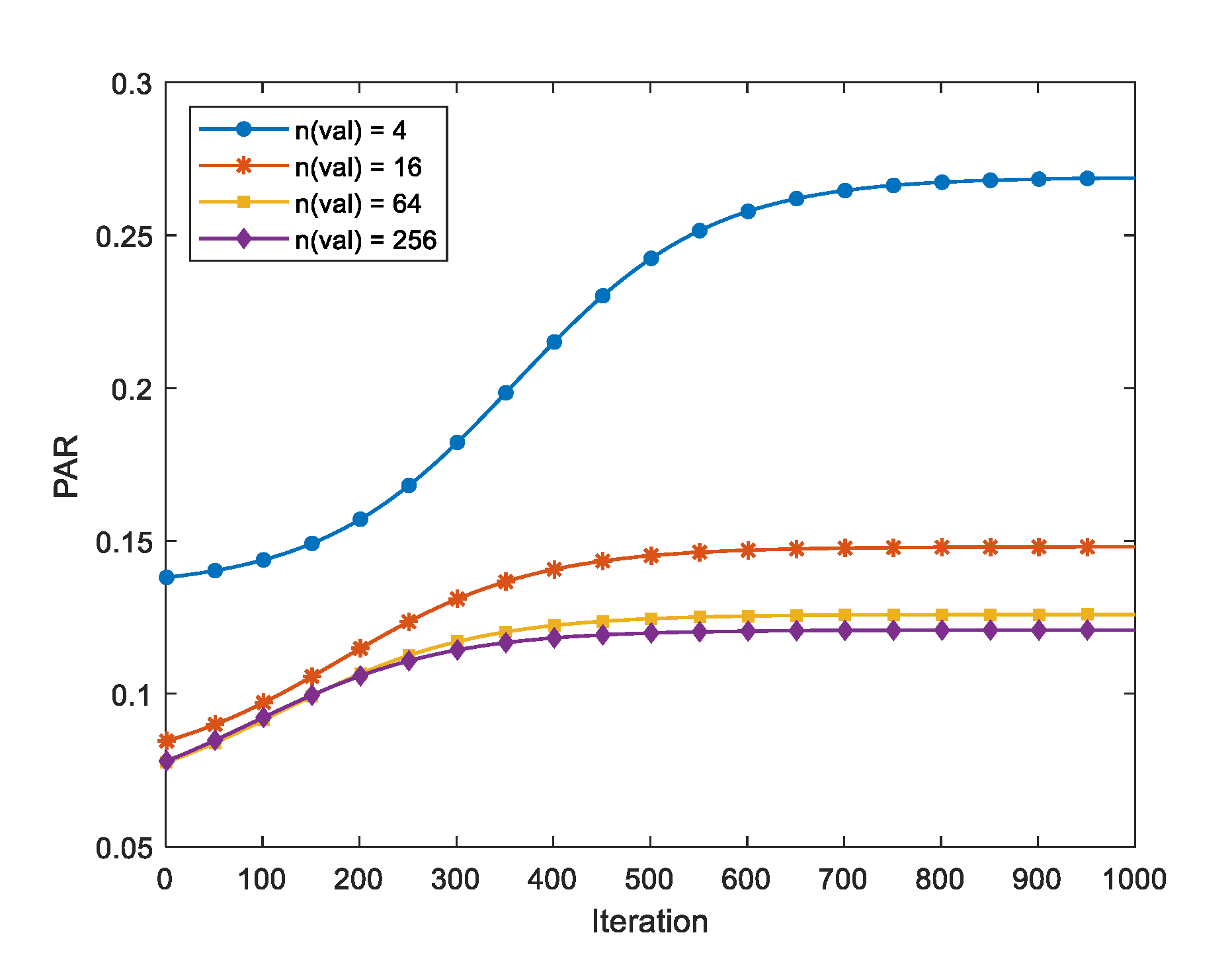
In Equation (8), HMCR is the HMCR value using the number of maximum iterations or the object value, and $n\left(val\right)$ is the number of variables changed by HS. Through this, if there is one variable, the PAR can have a value from 0.4404 to 0.8808, and if the variables are infinite, the PAR can have a value from 0.0596 to 0.1192.

The HMCR obtained in Equations (5) and (7) was increased as the iteration or the object value was reached, and this value was used to determine the PAR. As the HMCR value increased through the iteration of the HS algorithm, the probability of using the value stored in the HM increased, in which case the PAR value was increased to allow fine tuning of the variable. If there are many variables, several of them need not be adjusted at one time. Therefore, the number of variables was used to determine the value of PAR such that the more the number of variables, the lower was the PAR value. The resulting PAR values are shown in Figure 6.

Thus, the advanced PSF method can achieve appropriate HMCR and PAR without requiring additional memory, unlike the conventional PSF scheme. The advanced PSF scheme operates according to the number of HS maximum iterations or the object value of the HS, so that the maximum improvisations can be used for the HS algorithm.

3.4. Pitch Adjusting Bandwidth Dependent on the Object

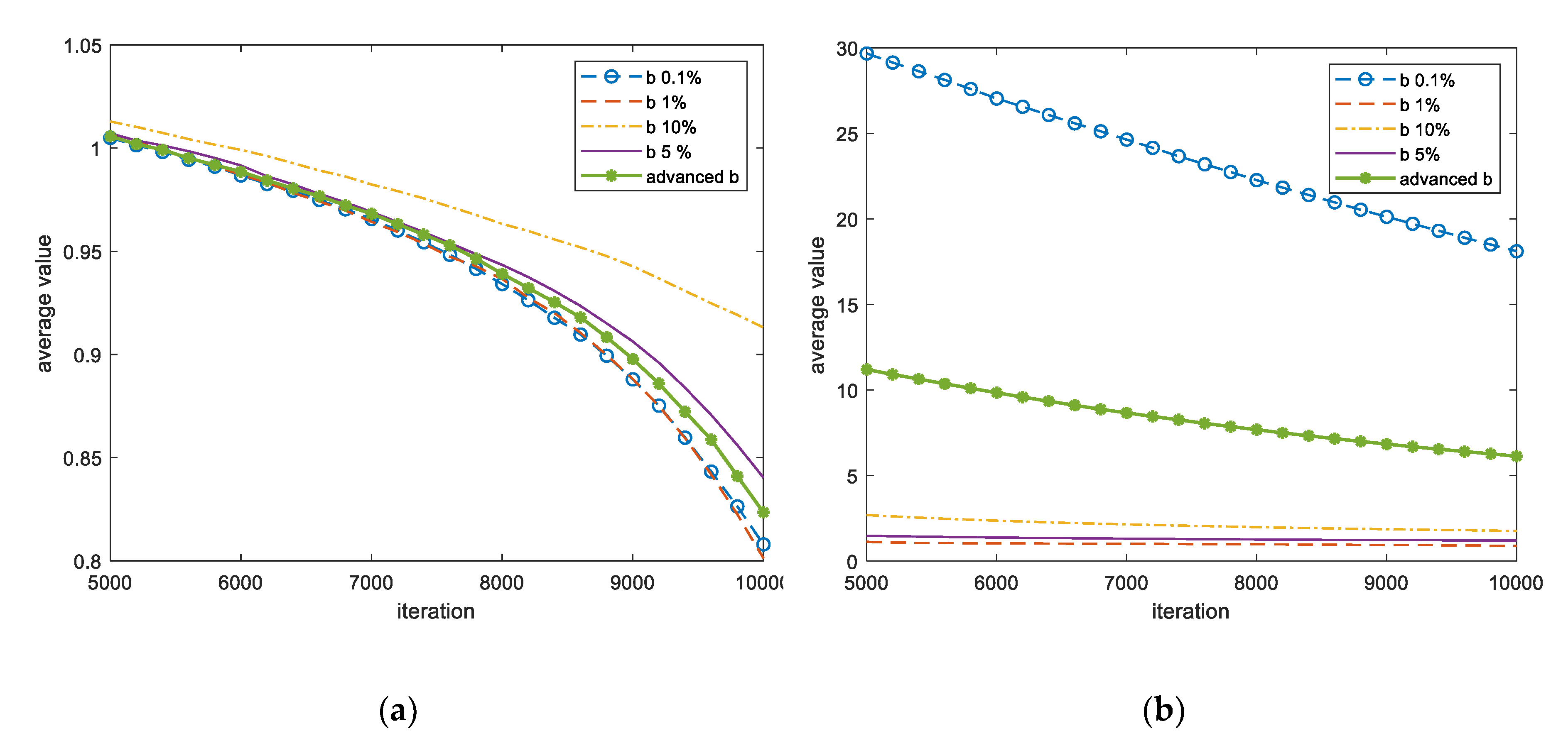
In addition, the pitch adjusting bandwidth was used to determine the maximum range of this adjustment level when using the existing value as the probability of HMCR and adjusting the value with the probability of PAR. However, this method was possible only when using an object, not when using iteration when defining an HMCR. In a typical HS, 0.1% of the full range was used when setting the adjustment range, $b$. However, depending on the problem given, the appropriate range was different, and in the case of a function, if the entire range is a different size, the appropriate adjustment range is also different. Due to this, there are various methods of determining pitch adjusting bandwidth [15], but most of them are determined by specifying the maximum and minimum values of the adjustment range in advance. Therefore, Equation (9) was proposed to obtain an appropriate adjustment range without specifying these values.

$b_{\mathrm{i}}$ is the pitch adjusting bandwidth used until the HS is iterated $\mathrm{i}$ times the HMS and then $\mathrm{i}+1$ times the HMS. Set $b$ to any value within the entire input range until the first time HS is repeated the same number of times as HMS. U and L are the maximum and minimum values of the entire problem input range; $Los{s}_i$ is the average of the HM results when HS is repeated $\mathrm{i}$ times the HMS; $Los{s}_{obj}$ is the object value, and $Los{s}_{start}$ is the mean of the function result stored in the HM immediately after performing the same number of times as HMS. In the case of repeating the same number of times as the first HMS, $Los{s}_0$ uses $Los{s}_{start}$.

$$\{\begin{array}{l}{b}_{\mathrm{i}}=\left(\mathrm{U}-\mathrm{L}\right)\times \frac{Los{s}_{i-1}-Los{s}_i}{Los{s}_{start}-Los{s}_{obj}}, {\mathrm{b}}_{\mathrm{i}}\ge \left(\mathrm{U}-\mathrm{L}\right)\times 0.0001\\ b_{\mathrm{i}}=\left(\mathrm{U}-\mathrm{L}\right)\times \left(1-\frac{Los{s}_{start}-Los{s}_i}{Los{s}_{start}-Los{s}_{obj}}\right)\times 0.1, else \end{array}$$

(9)

Figure 7 shows the results of the advanced PSF HS produced by HMCR using objects in the Griewank function. Even though the same function is shown in this figure, the optimum pitch adjusting bandwidth was different when the input range was different. The advanced $b$ obtained by Equation (9) proposed in this study did not produce the best value but showed good results.

In the newly designed method, changing the HMCR and the PAR requires the maximum number of iterations or the object value. Therefore, the case of using the maximum number of iterations is the iteration PSF scheme and the case requiring the object value is denoted the object PSF scheme. Applying this method to HS is equivalent to changing the “Calculate and Compare HM” box in Figure 1, Figure 2, Figure 3, Figure 4, Figure 5, Figure 6, Figure 7 and Figure 8.

4. Performance Comparison by PSF Type

4.1. Test in the Continuous Test Function

In the case of the conventional PSF method, the number of iterations required for HMCR and PAR to become 0 or 1 differs depending on the HMS. Therefore, the HMS was set to 50, which is relatively large compared to the number of variables, and the pitch adjusting bandwidth was set to 5% of each entire range. When using the conventional PSF method, the initial number of executions by fixing HMCR and PAR to 0.5 was set to 100 times. The result of performing various test functions [16,17,18,19,20] with the HS algorithm using the above settings and the method of manually setting the parameters of HS, using both the conventional PSF and the advanced PSF methods, were compared. When the advanced PSF scheme uses the maximum number of iterations, the number of maximum iterations was specified in units of 200 each.

4.1.1. Griewank Function

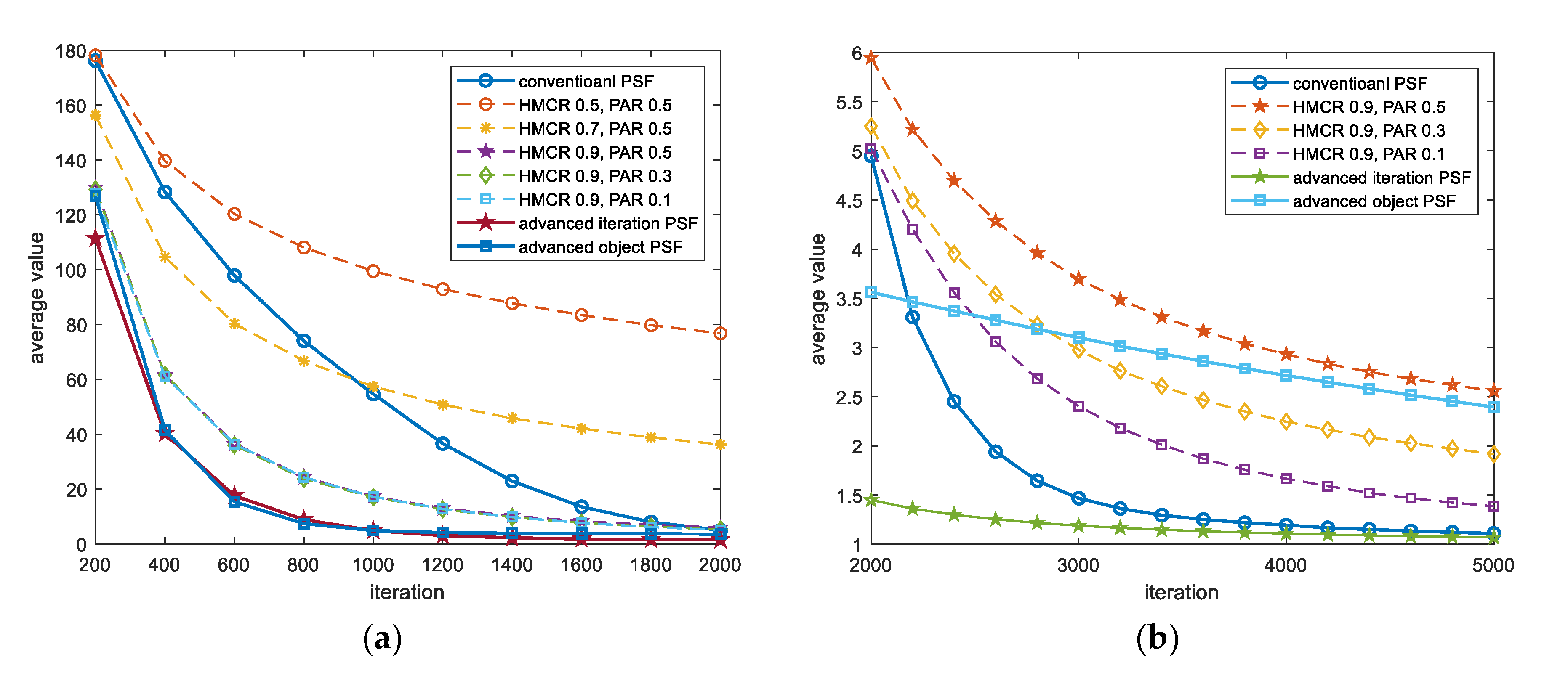
Figure 9 shows the average of 10,000 results using conventional PSF HS, fixed HMCR and PAR HS, and advanced PSF HS, when 16 variables are used with the Griewank function of Equation (10).

$$f\left(x\right)=f\left(x_1, \dots , x_n\right)=1+{\displaystyle \sum }_{i=1}^n\frac{x_i^2}{4000}-{\displaystyle \prod }_{i=1}^n\cos \left(\frac{x_i}{\sqrt{i}}\right)$$

(10)

The input range of the Griewank function is $x_i\in \left[-600, 600\right]$, and it has the minimum value in $f\left(x^{*}\right)=0, x^{*}=\left(0, \dots , 0\right)$, so 0 can be regarded as the target value. This value was designated as the target value when using the improved PSF scheme.

Figure 9a shows the iterations from 200 to 2000. In this case, after some iterations of HS, the results any kind of PSF HS show better results than those using fixed HMCR and PAR HS. However, if the number of iterations is not very high, it is better to use fixed HMCR and PAR than the conventional PSF scheme. On the other hand, the advanced PSF scheme always produces better results than other methods.

Figure 9b shows the iterations from 2000 to 5000. In this case, we can see that the conventional PSF scheme produced better results than the object PSF method from 2200 iterations. Since the Griewank function produced good results at a pitch adjusting bandwidth of 1 to 5% of the entire input range in 5000 iterations, the objective PSF method that did not use a good value of 5% shows relatively poor results compared to the iteration PSF method.

4.1.2. Salomon Function

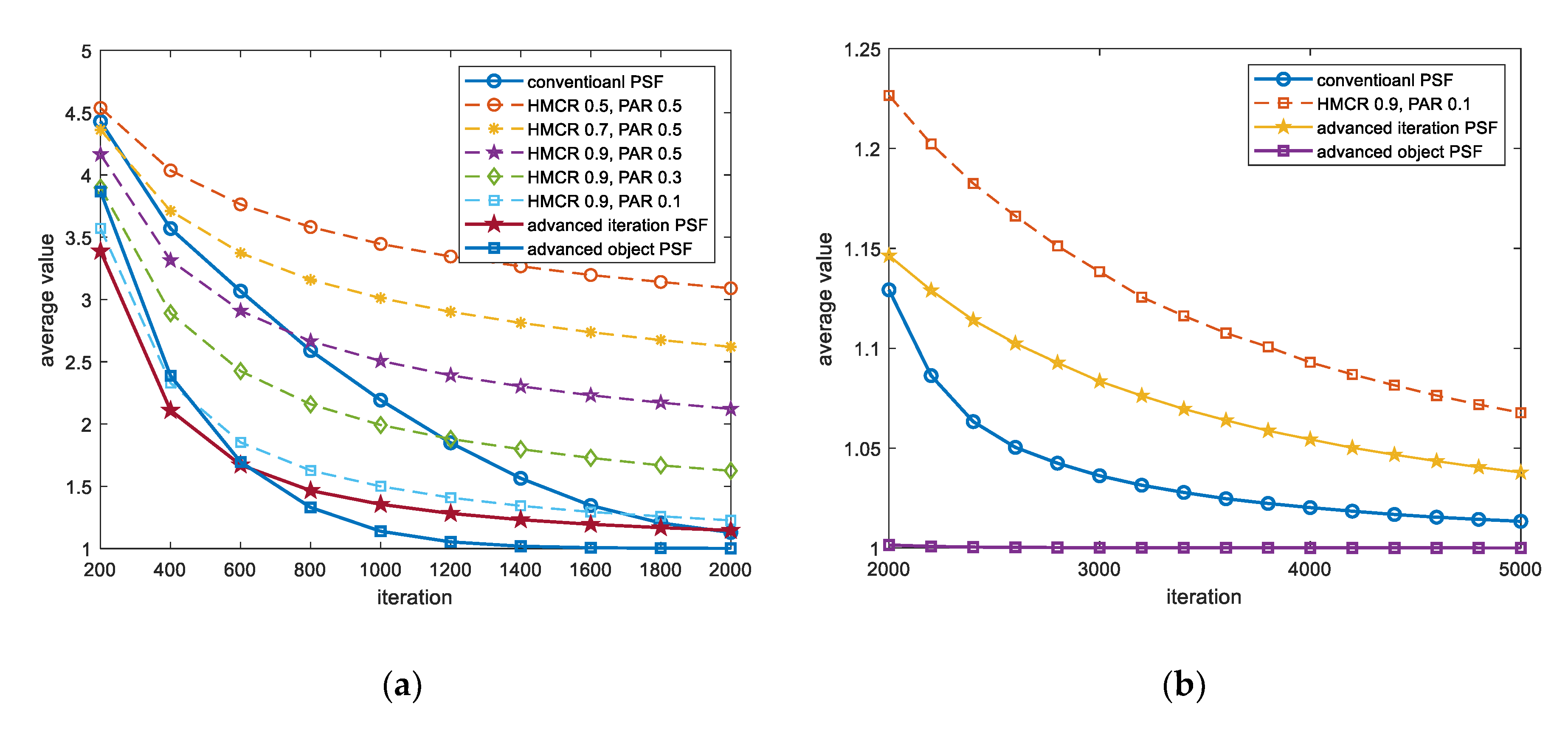
Figure 10 shows the average of 10,000 results using conventional PSF HS, fixed HMCR and PAR HS, and improved PSF HS when 16 variables were used with the Salomon function in Equation (11).

$$f\left(x\right)=f\left(x_1, \dots , x_n\right)=1-\cos \left(2\pi \sqrt{{\displaystyle \sum }_{i=1}^n{x}_i^2}\right)+0.1\sqrt{{\displaystyle \sum }_{i=1}^n{x}_i^2}$$

(11)

The input range of the Salomon function is $x_i\in \left[-100, 100\right]$, and it has the minimum value in $f\left(x^{*}\right)=0, x^{*}=\left(0, \dots , 0\right)$, so 0 can be regarded as the target value. This value was designated as the target value when using the improved PSF scheme.

Figure 10a shows the iterations from 200 to 2000. In this case, after some search iterations, the results using any kind of PSF HS show better results than those using fixed HMCR and PAR HS. However, if the number of iterations is not very high, it is better to use fixed HMCR and PAR than the conventional PSF HS. On the other hand, the advanced PSF HS always shows better results than other methods.

Figure 10b shows a graph of the iterations from 2000 to 5000. In this case, we can see that the conventional PSF scheme produced better results than the object PSF method from 3200 iterations. Since the Salomon function produced good results at a pitch adjusting bandwidth of 5 to 10% of the entire input range in 5000 iterations, the objective PSF method that did not use a good value of 5% shows relatively poor results compared to the iteration PSF scheme.

4.1.3. Periodic Function

Figure 11 shows the average of 10,000 results using conventional PSF HS, fixed HMCR and PAR HS, and improved PSF HS when 16 variables were used with the periodic function in Equation (12).

$$f\left(x\right)=f\left(x_1, \dots , x_n\right)=1+{\displaystyle \sum }_{i=1}^n{\sin }^2\left(x_i\right)-0.1e^{{\displaystyle \sum }_{i=1}^n{x}_i^2}$$

(12)

The input range of the periodic function is $x_i\in \left[-10, 10\right]$, and it has the minimum value in $f\left(x^{*}\right)=0.9, x^{*}=\left(0, \dots , 0\right)$, so 0.9 can be regarded as the target value. This value was designated as the target value when using the improved PSF scheme.

Figure 11a shows the iterations from 200 to 2000. Unlike other functions, the result of conventional PSF HS is quite good for the periodic function. This shows that near 2000 iterations, the conventional PSF scheme could produce better results than the iteration PSF scheme.

Figure 11b shows the iterations from 2000 to 5000. As can be seen in the figure, the conventional PSF HS yielded better results than the iteration PSF HS. The periodic function produced good results at 0.1% pitch adjusting bandwidth over the entire input range in 5000 iterations, so the objective PSF scheme shows relatively good results compared to other PSF methods with a value of 5%.

4.1.4. Three Types of PSF Scheme Comparison

Using 32 variables in the three types of functions mentioned above, the result of 20,000 iterations was obtained using three types of PSF HS, and the results were compared.

Table 1. Average of 10,000 results for 32 variables in each function using PSF-HS and suitable pitch adjusting bandwidths.

Function	PSF Type	4000 iter	8000 iter	12,000 iter	16,000 iter	20,000 iter
Griewank	Conventional	23.2639	4.4741	2.9851	2.3429	1.9419
	Iteration	2.0668	1.4455	1.2903	1.2084	1.1645
	Object	13.0668	7.8658	5.1469	3.7086	2.8577
Salomon	Conventional	6.8991	2.8425	2.0464	1.7192	1.5463
	Iteration	2.2150	1.4152	1.1541	1.0129	0.9207
	Object	3.9688	3.3026	2.7275	2.2429	1.8403
Periodic	Conventional	1.3657	1.1097	1.0789	1.0626	1.0523
	Iteration	1.0296	1.0004	1.0002	1.0001	1.0001
	Object	1.0004	1.0001	1.0000	1.0000	1.0000

shows the mean of collecting 10,000 results of PSF HS according to the number of iterations when the number of variables was 32. The bolded numbers in the table are the average of the best results among the PSF types for a given number of iterations. Except in the case of using the object PSF scheme, the HS calculation of each function used the suitable pitch adjusting bandwidth, using 5% for Griewank and Salomon and 0.1% for periodic. For the iteration PSF HS, each iteration used in the table was calculated using the target value. The other conditions are the same as those mentioned above.

In this case, the use of iteration PSF HS gave good overall results. This shows that using an iteration PSF scheme at the same pitch adjusting bandwidth yielded better results than using a conventional PSF scheme. When using the objective PSF HS, the periodic function provided the best results.

Table 2. Average of 10,000 results for 32 variables in each function using PSF-HS and unsuitable pitch adjusting bandwidths.

Function	PSF Type	4000 iter	8000 iter	12,000 iter	16,000 iter	20,000 iter
Griewank	Conventional	28.0128	7.3089	5.2085	4.3156	3.6455
	Iteration	9.7959	3.4818	1.5153	0.5534	0.0889
	Object	13.0668	7.8658	5.1469	3.7086	2.8577
Salomon	Conventional	6.8026	3.7045	3.2354	2.9802	2.8125
	Iteration	3.8990	3.1242	2.7194	2.4590	2.2816
	Object	3.9688	3.3026	2.7275	2.2429	1.8403
Periodic	Conventional	1.5800	1.1179	1.0898	1.0721	1.0620
	Iteration	1.5342	1.2988	1.2093	1.1578	1.1258
	Object	1.0004	1.0001	1.0000	1.0000	1.0000

shows the mean of collecting 10,000 results of PSF HS according to the number of iterations when the number of variables was 32. The bolded numbers in the table are the average of the best results among the PSF types for a given number of iterations. Except in the case of using the object PSF scheme, the HS calculation of each function used an unsuitable pitch adjusting bandwidth, using 0.1% for Griewank and Salomon and 5% for periodic. For the iteration PSF scheme, each iteration used in the table was calculated using the target value. The other conditions are the same as those mentioned above.

In this case, the use of the advanced PSF HS shows good results. The results using the conventional PSF HS as shown in Table 2 are worse than those in Table 1. On the other hand, the Griewank function using the iteration PSF HS shows poor results with fewer iterations but better results with many iterations. The appropriate pitch adjusting bandwidth varied according to the method of determining the HMCR, PAR, and the type of the problem. The more iterations of the Salomon function’s HS results, the better it is to use the object PSF rather than the iteration PSF scheme. This indicates that the iteration PSF HS results with poor pitch adjusting bandwidth were not good. In the periodic function, the results of the methods except the object PSF HS were not good. Moreover, in this case, the result of the conventional PSF HS was better than that of iteration PSF HS.

Other functions were used to compare PSF HS types. When performing HS, the HMS was 50, and the number of variables was 32. The pitch adjusting bandwidth was found to be a total of four cases using 0.1% of all three PSF schemes, and the use of advanced $b$ in the objective PSF method. When using conventional PSF HS, the initial number of iterations was set to 100 by fixing HMCR and PAR to 0.5. The functions used are shown in

Table 3. Test functions.

Function Name	Function	Input Range	Minimum
Sphere	$f\left(x\right)={\displaystyle {\displaystyle \sum }_{i=1}^n}{x}_i^2$	[−5.12, 5.12]	0
Rosenbrock	$f\left(x\right)={\displaystyle {\displaystyle \sum }_{i=1}^n}\left[100{\left(x_{i+1}-x_i^2\right)}^2+{\left(1-x_i\right)}^2\right]$	[−5, 10]	0
Rastringin	$f\left(x\right)=10n+{\displaystyle {\displaystyle \sum }_{i=1}^n}\left(x_i^2-10\cos \left(2\pi x_i\right)\right)$	[−5.12, 5.12]	0
Ackley	$f\left(x\right)=20+e-20e^{-0.2\sqrt{\frac{1}{n}{\displaystyle \sum }_{i=1}^n{x}_i^2}}-e^{\frac{1}{n}{\displaystyle \sum }_{i=1}^n\cos \left(2\pi x_i\right)}$	[−32, 32]	0
Happycat	$f\left(x\right)={\left({\Vert x\Vert }^2-n\right)}^{\frac{1}{4}}+\frac{1}{n}\left(\frac{1}{2}{\Vert x\Vert }^2+{\displaystyle {\displaystyle \sum }_{i=1}^n}{x}_i\right)+\frac{1}{2}$	[−2, 2]	0

, and the results are shown in

Table 4. Average of 10,000 results for 32 variables in each function using PSF HS.

Function	PSF Type	4000 iter	8000 iter	12,000 iter	16,000 iter	20,000 iter
Sphere	Conventional	7.3047	1.7931	1.1941	0.9677	0.8475
	Iteration	2.5973	0.7254	0.1530	0.0105	2.1888 × 10-4
	Object	9.0669	6.1348	3.8778	2.2569	1.1523
	Object + $b$	3.5976	2.1292	1.3533	0.9450	0.7000
Rosenbrock	Conventional	4.2053 × 105	1.9097 × 103	8.6170 × 102	6.2643 × 102	5.0953 × 102
	Iteration	2.4875 × 103	6.1813 × 102	2.7474 × 102	1.8004 × 102	1.3778 × 102
	Object	1.8541 × 104	1.1280 × 104	6.6921 × 103	3.8371 × 103	2.1353 × 103
	Object + $b$	1.1240 × 104	9.0852 × 103	7.5634 × 103	6.4223 × 103	5.5621 × 103
Rastringin	Conventional	46.1926	30.3153	26.3731	24.1580	22.5746
	Iteration	25.7417	13.8458	11.2223	8.9907	7.5238
	Object	42.7380	35.5440	34.2143	33.1040	31.9219
	Object + $b$	25.5767	24.9163	24.3740	23.9071	23.4128
Ackley	Conventional	9.7717	6.2214	5.2261	4.7196	4.3750
	Iteration	7.0990	5.0225	4.0665	3.4594	3.0939
	Object	16.7124	7.5771	5.0366	4.6922	4.4424
	Object + $b$	16.7367	6.9600	1.4705	1.2630	1.2277
Happycat	Conventional	0.5862	0.5011	0.4521	0.4153	0.3820
	Iteration	0.3783	0.2216	0.1605	0.1282	0.1076
	Object	0.3581	0.2064	0.1548	0.1303	0.1164
	Object + $b$	0.3715	0.2116	0.1553	0.1295	0.1144

. Table 4 shows the mean of collecting 10,000 results of PSF HS according to the number of iterations when the number of variables was 32. The bolded numbers in the table are the average of the best results among the PSF types for a given number of iterations.

As shown in Table 4, in most cases it is better to use the advanced than conventional PSF scheme. The iteration PSF method shows the best results in almost all cases. On the other hand, in the case of object PSF HS, the result varied greatly depending on the type of function. The use of advanced $b$ had a significant effect on certain functions. This shows that it is better to set the pitch adjusting bandwidth of the function to a different value than 0.1%.

4.2. Test in Discrete Test Function

We compared the advanced PSF HS results with those using the test function from the conventional PSF scheme.

$$f\left(x\right)={\displaystyle \sum }_{i=1}^5{\left(x_i-i\right)}^2$$

(13)

The input range of Equation (13) is $x_i\in \left\{1, 2, \dots , 10\right\}$ as discrete values, and the minimum value is $f\left(x^{*}\right)=0, x^{*}=\left(1, 2, 3, 4, 5\right)$. When the HS algorithm is performed using this equation, the HMS is equal to 25 and $\pm 1$ is set if there is a change due to the PAR. Unlike the conventional PSF scheme, one of the advanced PSF methods can be used only when the number of executions is determined. Therefore, the maximum number of iterations was set to 500 and 1000, and when the minimum value of 0 was obtained, a total of 100,000 results were collected, and the number of iterations necessary for the minimum value was measured.

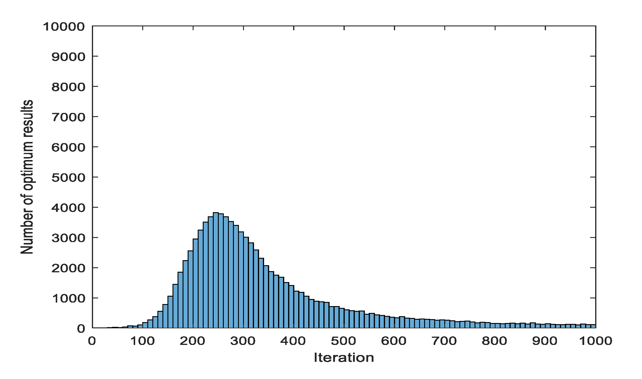
Figure 12 shows the results of Equation (13) using conventional PSF HS. The initial number of iterations required for the existing PSF configuration was specified as 50. In the case of using the conventional PSF scheme, it is not necessary to specify the number of maximum iterations. After iterating 1000 times, the number of cases exceeding a certain number of executions was checked, and the average and deviation of the number of executions were checked.

Of the 100,000 results, a total of 10,877 results had no minimum value found within 1000 iterations. Of the 100,000 results, a total of 23,424 results had no minimum value found within 500 iterations. If the minimum value could not be found within 1000 iterations, it was processed as 1000 iterations and the following calculation was made. The average number of iterations was 412.6820 and standard deviation was 258.3526. Since the values of HMCR and PAR, which are problems of the conventional PSF method, were fixed to 0 or 1, the number of iterations was increased to find the minimum value, or the minimum value could not be found. For this reason, the number of executions was more skewed than the normal distribution, and there were many cases where the minimum value was not found within 1000 iterations.

Figure 13a shows the results with 1000 iterations using advanced PSF HS that specifies the maximum number of iterations. In the total of 10000 results, the minimum value was not found within 500 iterations of 4590. The average iteration count was 396.0212, the standard deviation was 73.9069, and the maximum iteration count was 637.

Figure 13b shows the results with 500 iterations using advanced PSF HS that specifies the maximum number of iterations. However, for comparison, the histogram is drawn with the same iterations. The average iteration count was 287.8152, and the standard deviation was 49.8264. In one case, the minimum value was not found in 500 iterations.

When using the method of specifying the maximum iteration count for the advanced PSF scheme, there may be problems with specifying the maximum iteration number. However, if the appropriate maximum iteration number was specified, the results were better that of the conventional PSF HS.

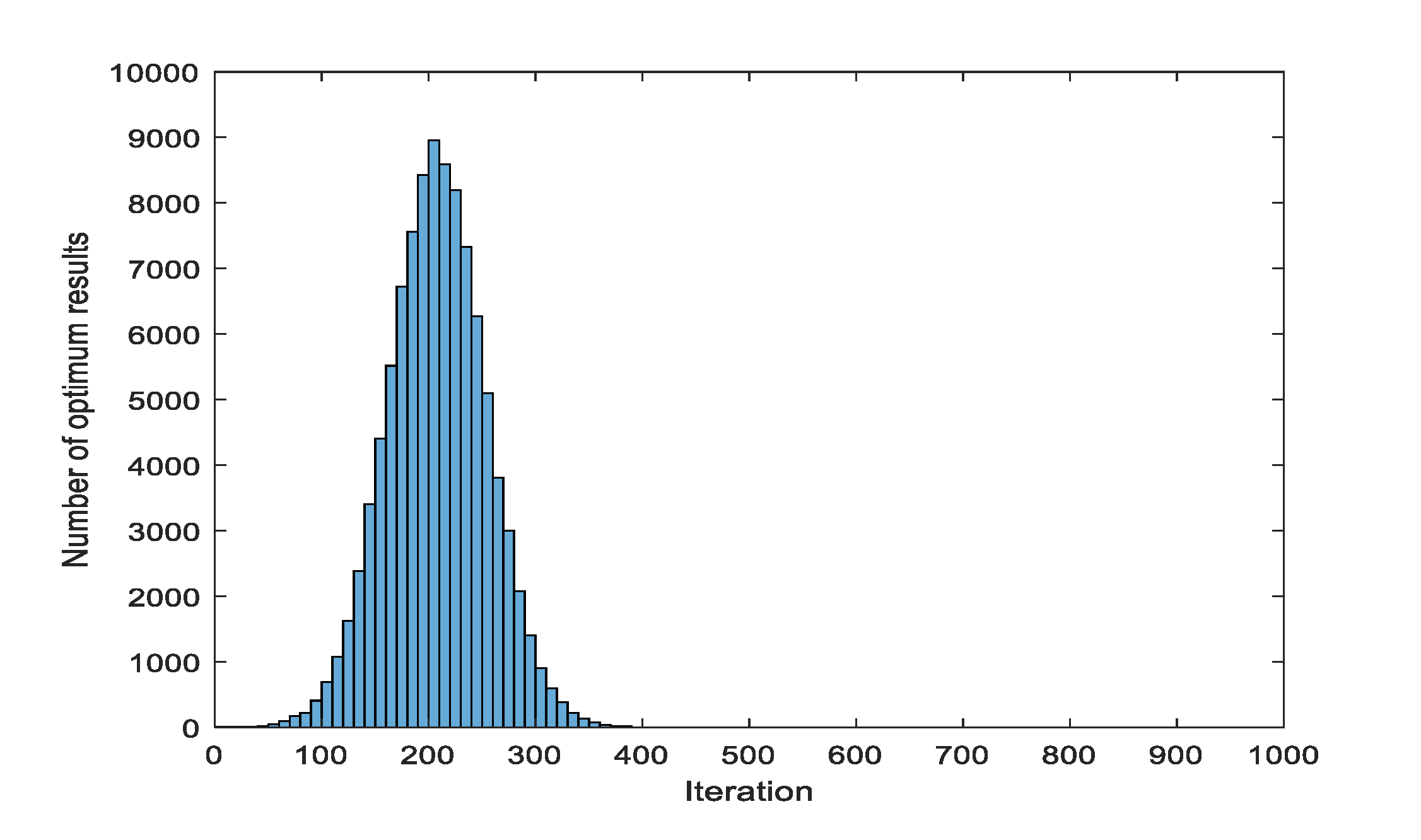
Figure 14 shows the results using advanced PSF HS to specify the object values. The average iteration count was 207.6412, the standard deviation was 46.1493, and the maximum iteration count was 445.

If the method of specifying the target value for the advanced PSF HS was used, the result was better than that with the conventional and advanced PSF schemes that specify the maximum number of iterations.

5. Conclusions

As the HS algorithm progresses, the conventional PSF method that automatically generates HMCR and PAR, called harmony memory consideration and pitch adjustment, which are necessary parameters for using the HS algorithm, can be changed. However, the conventional PSF method has the problem that there is no change after the parameter to be determined converges to a specific value. To solve this problem, an advanced PSF method was designed and verified through various test functions in this study.

In the conventional PSF scheme, the larger the HMS, the smaller the rate of change of the HMCR and PAR is. Therefore, the HMS must be large to slow the fixation to a value of 0 or 1. In addition, conventional PSF scheme needs to use additional memory to store the number of iterations that the HMCR and PAR are performed, but the advanced PSF scheme is not limited by the HMS and can be calculated without the need for additional memory.

Unlike the conventional PSF and advanced PSF schemes in the same n-dimensional test function, the performance of the advanced PSF method was better when the number of variables that perform HS increased, and a greater number of iterations ensured better results. The performance of the advanced PSF scheme was thus comparable to or better than the conventional PSF scheme.

Therefore, for the HS algorithm using the advanced PSF, the HMS did not pose problems. In addition, if the object value could not be determined, the maximum number of iterations was used, whereas if the object value was set, the advanced PSF scheme using the object value could easily produce the best result or an equivalent result to the HS algorithm, thus avoiding the need to find the best HMCR and PAR. This advanced PSF method was therefore expected to be applicable to various fields that use the HS algorithm.