Abstract
A decentralized control scheme is developed in this paper based on an improved active disturbance rejection control (IADRC) for output tracking of square Multi-Input-Multi-Output (MIMO) nonlinear systems and compared with the decoupled control scheme. These nonlinear MIMO systems were subjected to exogenous disturbances and composed of high couplings between subsystems, input couplings, and uncertain elements. In the decentralized control scheme, it was assumed that the input couplings and subsystem couplings were both parts of the generalized disturbance. Moreover, the generalized disturbance included other components, such as exogenous disturbances and system uncertainties, and it was estimated within the context of Active Disturbance rejection Control (ADRC) via a novel nonlinear higher order extended state observer (NHOESO) from the measured output and canceled from the input channel in a real-time fashion. Then, based on the designed NHOESO, a separate feedback control law was developed for each subsystem to achieve accurate output tracking for given reference input. With the proposed decentralized control scheme, the square MIMO nonlinear system was converted into approximately separate linear time invariant Single-Input-Single-Output (SISO) subsystems. Numerical simulations in a MATLAB environment showed the effectiveness of the proposed technique, where it was applied on a hypothetical MIMO nonlinear system with strong couplings and vast uncertainties. The proposed decentralized control scheme reduced the total control signal energy by 20.8% as compared to the decoupled control scheme using Conventional ADRC (CADRC), while the reduction was 27.18% using the IADRC.
1. Introduction
Most industrial processes are modeled as nonlinear MIMO systems, which include high nonlinear couplings between subsystems and are subjected to both internal uncertainties and exogenous disturbances. Therefore, it is necessary to design a controller that is relatively simple to be implemented. The parameters of the required controller should be easy to be tuned to accommodate the operating conditions. Initial presentations of the active disturbance rejection control (ADRC) were based on a nonlinear version of the extended state observer (ESO) [1] and were subsequently streamlined and parameterized in Reference [2].
1.1. Active Disturbance Rejection Control
Active disturbance rejection control is an innovative strategy; its fundamental principle lies in augmenting the state-space model of the system with a supplementary fictitious first-order differential equation. This fictitious equation defines all the undesirable system uncertainties, dynamical properties, and external disturbances, denoted as a “generalized disturbance” [3]. This fictitious state, as well as the states of the dynamical plant, is estimated in a real-time manner by the extended state observer (ESO). which is the central part of the active disturbance rejection control (ADRC) [4]. It achieves an immediate and dynamic estimation and elimination of the generalized disturbance by returning its prediction to the control port with basic calculations using control law with output feedback. With ADRC, controlling a sophisticated uncertain nonlinear plant is transformed approximately into a simple linear time-invariant system [5,6]. The supremacy that makes it such a powerful control instrument is that it is a model-free method, instead of a model-based technique. Mainly, ADRC comprises of an ESO, a nonlinear state error feedback (NLSEF), and a tracking differentiator (TD), as shown in Figure 1, where is the desired signal, is the transient profile, is the relative degree, is the control input, and is the expanded estimated vector, which includes the predicted states of the system and the predicted generalized disturbance .
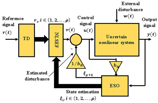
Figure 1.
Structure of the conventional SISO active disturbance rejection control (ADRC) configuration, is the nonlinear system’s relative degree.
Numerous engineering control challenges have been adequately resolved over the past 20 years through the successful application of ADRC. These include a high purity distillation column [7], the tension and velocity regulations in web processing lines [8], high-performance motion control [9], DC-DC power converters [10], chemical processes [11], vibrational MEMS gyroscopes [12], hysteresis compensation [13], fault diagnosis [14], non-circular turning processes [15], high pointing accuracy and rotation speed [16], omnidirectional mobile robot control [17], the control of model-scale helicopters [18], flexible-joint manipulator control [19], and differential drive mobile robots [5]. More recently, manufacturers that have successfully adopted ADRC technology include Texas Instruments Inc., which utilized ADRC in its motion control chips (InstaSPIN™-MOTION) [20]. Parker–Hannifin Corporation recently adopted ADRC over its production lines at an extrusion plant and halved its energy usage [21]. Finally, the National Superconducting Cyclotron Laboratory in the United States deployed ADRC in some high-energy particle accelerators for the regulation of electromagnetic fields [22].
1.2. Related Works
For controlling MIMO systems with disturbances and uncertainties, several control techniques were examined in the literature. In Reference [23], a decoupling control is proposed based on the decoupler matrix and the improved active disturbance rejection control. In Reference [24], robust tracking control of the MIMO system is presented and the second order sliding mode control (SMC) is used to establish the desired tracking. In Reference [25], a Lyapunov model-reference adaptive control for MIMO linear systems is designed for minimum phase systems with relative degree one. In Reference [26], the problem of almost disturbance decoupling is discussed for a class of MIMO nonlinear systems with external time-varying disturbances. In Reference [27], MIMO controllers are designed, which maximize the maximum amplitude of the sinusoidal input, for which the corresponding periodic solutions are guaranteed to be stable. In Reference [28], adaptive output feedback control is designed for MIMO systems under the framework of multirate sampled data control. In Reference [29], systematic synthesis of a fully reliable or partially reliable decentralized MIMO Proportional-Integral-Derivative (PID) controller is designed to achieve closed-loop stability. In Reference [30], adaptive tracking control is designed for uncertain MIMO nonlinear systems with non-symmetric input constraints. In Reference [31], derivative-integral terminal SMC is proposed for robust output tracking of uncertain MIMO systems. In Reference [32], a novel control strategy is developed for the trajectory tracking control of MIMO systems with hard constraints and uncertainties. In Reference [33], adaptive control scheme is investigated with unknown parameters and is developed for MIMO nonlinear time delay systems. In Reference [34], equivalent control-based SMC for MIMO uncertain linear Markovian jump systems is designed, which guarantees the system’s stochastically asymptotical stability. In Reference [35], adaptive control using multiple models with second level adaptation is designed for MIMO coupled systems. In Reference [36], a robust output regulation is proposed for invertible nonlinear MIMO systems based on the nonlinear internal model. In Reference [37], a full-order terminal SMC is designed for MIMO systems with unmatched uncertainties. In Reference [38], a tracking control problem of a class of MIMO nonlinear systems under asymmetric full-state constraints is proposed using dynamic surface control. In Reference [39], adaptive disturbance rejection tracking control is proposed with the asymptotically converging output tracking errors for MIMO nonlinear Euler–Lagrange systems, with unknown time-varying disturbances under input saturation. Authors in Reference [40] proposed a robust sliding mode controller of uncertain MIMO nonlinear systems with external disturbance rejection capabilities. The work in Reference [41] offered a novel sliding mode disturbance observer (SMDO) with finite-time convergence. Authors in Reference [42] constructed an output feedback sliding mode controller for MIMO systems of any relative degree. Moreover, the new high order sliding mode (HOSM) control algorithm is concluded in Reference [43], which guarantees finite-time stabilization of the linear MIMO system and rejects bounded matched and ”vanishing” unmatched disturbances of a particular type. Authors in Reference [44] proposed a MIMO nonlinear anti-disturbance compensator based on the linear extended state observer (LESO) for an unmanned aerial vehicle with exogenous disturbances and uncertainties. Authors in Reference [45] demonstrated an extended high-grain observer as a disturbance estimator in combination with a dynamic inversion technique with an application on nonlinear MIMO systems.
In Reference [46], a fuzzy adaptive control approach, based on a new kind of fuzzy adaptive observer, is designed for nonlinear MIMO systems. The authors in Reference [47] presented a fuzzy-based disturbance observer for MIMO nonlinear systems and demonstrated it for the output feedback control of a permanent Magnet Synchronous Motor (PMSM). In Reference [48], an adaptive fuzzy controller for uncertain MIMO nonlinear systems with unknown dead-zones and a triangular control is proposed. In Reference [49], an intelligent adaptive control system is proposed for MIMO uncertain nonlinear systems. In Reference [50], an adaptive fuzzy decentralized control is designed for interconnected nonlinear systems. In Reference [51], an adaptive fuzzy tracking control is designed for uncertain nonlinear MIMO systems with the external disturbances. A novel adaptive Neural Network(NN) control is proposed in Reference [52] for uncertain MIMO nonlinear time-delay systems. In Reference [53], an adaptive fuzzy backstepping dynamic surface control output feedback control is designed for MIMO strict-feedback nonlinear systems with time-varying disturbances and unmeasured states. A neural network adaptive controller is suggested in Reference [54] for MIMO systems with unknown nonlinear function. In Reference [55], two stable adaptive neural control schemes for MIMO nonlinear systems are presented. The authors in Reference [56] developed a novel data-driven multivariate nonlinear controller design for MIMO nonlinear systems via virtual reference feedback tuning and neural networks. In Reference [57], a prescribed performance tracking control is designed for MIMO nonlinear systems with immeasurable states and unknown control direction. Finally, the authors in Reference [58] designed an event-triggered adaptive fuzzy control for MIMO switched nonlinear systems to estimate the whole information of the system states.
Although the previously mentioned studies of adaptive control strategies have a lot higher influence and fundamentally improve the capability of a feedback control system in managing uncertainties outside robust control, this improvement is compelled by the variation rates of the uncertain coefficients. Moreover, the performance exacerbates immediately if these variation rates exceed a specific boundary. These conventional strategies in dealing with deterministic adaptive control have some natural limitations [59,60]. Most surprisingly, if the unknown parameters fluctuate in a complicated fashion, it may be quite challenging to build up a “continuously parameterized” class of contender controllers. Furthermore, regular adjustment over some undefined time frame may be a strenuous task. These matters become exceptionally cruel if robustness and superior performance are in demand. In this manner, the strategy of adaptive control methods incorporates a generous number of specific steps and often depends on experimentations [39]. Far from adaptive control, the sliding mode control approach is thought to be one of the proficient techniques to build powerful controllers for highly complicated nonlinear plants with the opportunity of stabilizing some nonlinear systems that can’t be stabilized by continuous state feedback laws. The significant obstruction in the success of these methods is the chattering phenomenon, which makes the actuators needed to adapt to the high-frequency control activities that could produce premature wear and tear.
In this work, for controlling highly coupled MIMO nonlinear systems with external disturbances, internal unmodelled dynamics, and uncertainties, a proposed control scheme was proposed, namely, the decentralized control scheme based on improved ADRC (IADRC) configuration. This ADRC scheme is systematic and achieves, in large scale, the estimation/cancelation of the generalized disturbance in a single shot. The proposed scheme does not need extensive parameter tuning as in the case of neural network-based adaptive control techniques. Moreover, the chattering in the control signal, a common phenomenon in the sliding mode control, was avoided in the proposed scheme. Finally, the proposed decentralized control scheme is a direct technique, which means it estimates/cancels the generalized disturbance in a real-time manner without a need for a decision from an inference engine, as in the case of adaptive fuzzy control with so many fuzzy-rules that need to be developed and stored in a database.
1.3. Paper Contribution
The contributions of this paper are twofold. First, a decentralized control scheme based on IADRC configuration was proposed to deal with the input couplings and subsystem couplings, where they are all refined into the generalized disturbance. This generalized disturbance was reflected in the output signal, and a novel ESO was designed to measure the generalized disturbance. Second, in the proposed decentralized control scheme, the generalized disturbance was estimated from the output signal through a nonlinear higher order ESO (NHOESO), which is different from the conventional ESOs due to two main features: (1) possessing a nonlinear error-correcting term to satisfy the rule, “big error, small gain or small error, big gain”, (2) having one more augmented state for better estimation of the generalized disturbances, specifically with higher-order derivative disturbances.
1.4. Paper Organization
The rest of the paper is structured as follows. In Section 2, the problem statement is presented and sheds light on the formulation of the generalized disturbance for the MIMO nonlinear system. The decoupled control scheme is explained in Section 3, while the main results are offered in Section 4; these include the proposed decentralized control scheme, the improved ADRC (IADRC), and the closed-loop system stability analysis. In Section 5, a very complicated hypothetical MIMO uncertain nonlinear system is considered as a study example to investigate the performance of the proposed decentralized control scheme. Finally, the paper is concluded in Section 6.
2. Problem Statement
Consider a MIMO nonlinear system given as:
The above system belongs to a class of a partial exact feedback linearizable system if the relative degree is less than the order of the MIMO nonlinear system n, where the control input is defined as , the measured output for the MIMO system is defined as , is the exogenous disturbance, the state vector of Equation (1) is denoted as, is the state vector of the system, is the total relative degree,, is the unknown system function, which includes system uncertainties, exogenous disturbances, and any unwanted dynamics, and is the input gain function for . The internal dynamics of the plant (Equation (1)) is described as , where is the unknown internal dynamics function.
Consider the state vector of the i-th subsystem, denoted as , . Let the coefficient be approximate of in the system with a ±50% zone [61,62], which then means Equation (1) can be described as,
The generalized disturbance , of the nonlinear MIMO system in Equation (1) is expressed as:
Figure 2 illustrates the system given in Equation (2), considering the generalized disturbance in Equation (3).
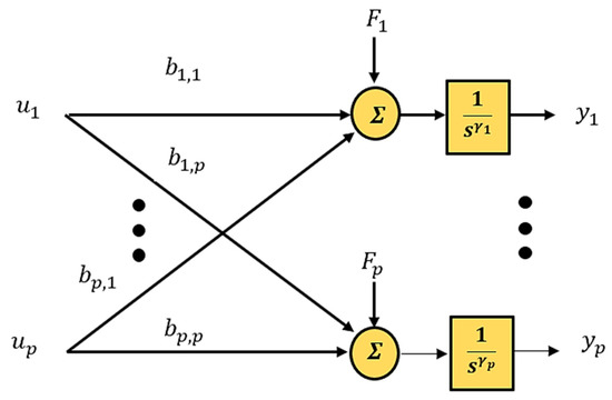
Figure 2.
Generalized disturbance representation for the MIMO nonlinear system.
It is necessary to design a controller for the MIMO system of Equation (1), which provides the following:
- Disassociation of the state couplings.
- Disassociation of the input couplings.
- Rejects the effect of the generalized disturbance, , on the outputs.
- Maintaining an acceptable performance during both transient and steady-state responses.
3. Decoupled Control [23]
In this control scheme, the controller was applied after adding a decoupler element between the ADRC and the nonlinear MIMO system. In recall Equations (2) and (3), the simplified model is expressed as,
The matrix form of Equation (4) is given as,
where is a non-singular input gain matrix and its inverse matrix is expressed as:
The proposed decoupler element used in this scheme is given as [23]:
By substituting the decoupler (Equation (7)) element in the system model (Equation (5)), we get
This leads to the following decoupled model,
This model can be expressed as,
Let . Additionally, let . The subsystem (Equation (9)) can be written as:
The virtual control signal in Figure 3 was generated according to the following formula (see Figure 1):
where is the estimation of the generalized disturbance of (Equation (3)), produced by a suitable designed ESO for this purpose. The uncertain nonlinear MIMO system of Equation (4) was converted into uncertain nonlinear systems, as expressed by Equation (10). The nominal control signal is a nonlinear combination of the tracking error and can be described as follows:
where is any nonlinear combination function with a sector bounded feature and satisfies (0) = 0 and is the tracking error vector, defined as The tracking error is defined as , for , where is the derivative of the reference signal , and is an estimation of the state , produced by a suitable designed ESO.
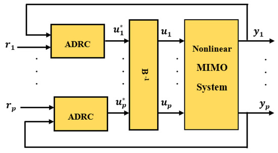
Figure 3.
The decoupled ADRC control scheme, where each ADRC block involves a SISO connection of a tracking differentiator (TD), nonlinear state error feedback (NLSEF), and an extended state observer (ESO), as in Figure 1 [23].
4. Main Results
The proposed decentralized control scheme is presented in this section. The IADRC was aimed to serve the intended functions of the proposed decentralized control scheme for MIMO nonlinear uncertain systems. Finally, the proposed control scheme was validated theoretically by demonstrating the closed-loop system’s stability analysis.
4.1. The Proposed Decentralized Scheme Based on ADRC
The decentralized control technique was proposed to control the nonlinear MIMO system given in Equation (2). This method utilizes the IADRC paradigm due to its high robustness against the effects of nonlinear coupling, inherent uncertainties, and exogenous disturbances, which are all estimated and canceled in an online fashion by the ESO.
In this control scheme, the nonlinear-coupled MIMO system in Equation (1) was converted to multi single-loop linear time-invariant SISO systems by treating the coupling input as a component of the generalized disturbance. By modifying Equation (1), this gives:
The generalized disturbance , including the coupling inputs, is given by:
Finally, the nonlinear MIMO system can be expressed in the simplified model, given as:
Let . Additionally, let . The subsystem (Equation (15a)) can be written as:
Figure 4 illustrates the system given in Equation (15a) and considers the generalized disturbance of Equation (14). Figure 5 shows the decentralized ADRC scheme for controlling the nonlinear MIMO system (Equation (15)). In this case, the control signals were produced in the same way as in Equation (11), i.e.,
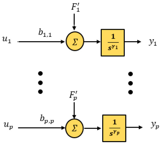
Figure 4.
Generalized disturbance representation for the decentralized ADRC scheme.
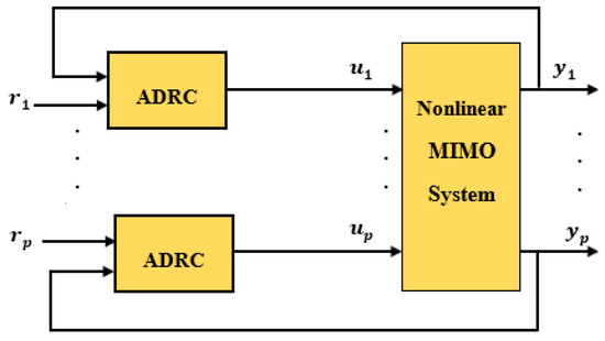
Figure 5.
The proposed decentralized ADRC control scheme, where each ADRC block involves a SISO connection of TD, NLSEF, and ESO, as in Figure 1.
4.2. The Improved ADRC (IADRC)
The structure of the IADRC that was used in the proposed control scheme for MIMO uncertain nonlinear systems was the same as that of the conventional ADRC (CADRC), with the same units of conventional TD and an NLSEF, except for the conventional linear ESO (LESO), which was replaced by a novel nonlinear higher order ESO (NHOESO). The dynamical structure of the TD is considered as [62]:
where , is a design parameter and an application-dependent parameter, set accordingly to speed up or slow down the transient profile, , and is the output of the TD. The NLSEF has the following nonlinear error function [62]:
where , , , and are design parameters and, usually, indicates how wide the linear part is and . With proper selection of these parameters, the closed-loop tracking error could diminish (approaching 0) in a very short time. The novel NHOESO is proposed as follows:
where the vectors and are the observed model states and is the estimated generalized disturbance, is the bandwidth of the NHOESO of the i-th subsystem, , and and are the design parameters of the NHOESO. They were selected such that the following matrix was Hurwitz.
On the other hand, the nonlinear function , was designed as in Reference [63]:
where are positive design parameters and is the estimation error, defined as .
4.3. Closed-Loop Stability Analysis
The stability of the closed-loop system with the proposed decentralized control scheme and the IADRC is considered in the following theorem. Before proceeding with the stability analysis of the closed-loop system, the following two assumptions were required.
Assumption 1.
There is a stable NHOESO given, as in Equation (19), which produces the estimated statesandand the estimated generalized disturbance. These estimated states and the estimated generalized disturbance approach respectively asto the states, and a generalized disturbanceof the MIMO uncertain nonlinear system, expressed in Equation (10), i.e., withand.
Assumption 2.
There is a convergent TD given as in Equation (17), which generates a profileandfor the reference signal with minimum MSE. These trajectoriesapproach the reference trajectoryforas, i.e.,
Theorem 1.
Closed–Loop Stability.Given the MIMO nonlinear uncertain system of Equation (10), which has a linearization control law (LCL)of the form,
whereis given as:
with, whereis a even nonlinear gain function andis the closed-loop tracking error. If Assumptions 1 and 2 hold, then the closed-loop system is asymptotically stable, i.e.,
Proof.
The closed-loop tracking error between the reference profile of the TD and the corresponding estimated states of the MIMO nonlinear system is given as:
If Assumptions 1 and 2 hold, then the tracking error can be written as:
For the nonlinear plant of Equation (15), the states can be expressed in terms of the system output as:
Substituting Equation (29) in Equation (28) yields,
differentiating both sides of Equation (30) which results in
It yields the following dynamics for the tracking error
This, together with Equation (15b), gives:
Substituting Equation (25) in Equation (33), we get,
Based on Assumption 1, it follows that
The dynamics of the tracking error given in Equation (35), together with the control law designed in Equation (26), are written as:
with . The dynamics given in Equation (36) can be represented in matrix form as:
where,
,, , and . The characteristic polynomial of is given by:
The NLSEF controller adopted in this study utilizes the function given in Equation (18), which can be rewritten as a function of as:
with and , where
which is an even positive function. The design parameters of Equation (41) are chosen to guarantee that the roots of the polynomial Equation (39) have strictly negative real parts, i.e., a stable (Hurwitz) polynomial. □
5. Numerical Simulations
To show the performance of the proposed decentralized control scheme based on an IADRC for MIMO systems, consider the following MIMO uncertain nonlinear system:
where and are the outputs, and are inputs, is the external state vector, and is the internal state of Equation (42). , , ,,, and belong to , and the unknown functions are:
Suppose that the exogenous disturbances and the reference signals are as follows: The initial values of the model are taken as follows.
Two ADRC Configurations will be used in the simulations for the proposed decentralized control scheme. The difference between them is the type of ESO used to estimate the generalized disturbance and the nonlinear system’s states. These configurations are:
1. First configuration: The Conventional ADRC (CADRC)
The CADRC consists of the following units:
- Conventional TD, described by Reference [62]:where , is an application-dependent design parameter and it is set accordingly to speed up or slow down the transient profile.
- fal-based control law, given as:where is the tracking error and are design parameters.
- The LESO, given as follows [62]:where the vectors and are the observed model states, are the estimated generalized disturbance, and , is the bandwidth of the NHOESO of the i-th subsystem.
2. Second configuration: The Improved ADRC (IADRC)
The IADRC consists of the following units:
- Conventional TD is given by Equation (43).
- fal-based control law given by Equation (44).
- A novel NHOESO, proposed as:where the vectors and are the observed model states, are the estimated generalized disturbances, , are design parameters, and is the bandwidth of the NHOESO of the i-th subsystem. The nonlinear function is designed as in Reference [63]:withwhere are positive design parameters and is the estimation error.
5.1. Results of the Decoupled ADRC Control Scheme [23]
The input gain matrix, then . The proposed decoupler element used in this scheme given in Equation (7) is found as:
Then, the suggested feedback control laws and are formulated, as in Reference [23]:
where , is a design parameter and the function is defined as:
The virtual control signals in Equation (49) and indicated in Figure 3 is derived from the fal-based control law given in Equation (44). The desired transient trajectories and are generated from the reference signals via the tracking differentiators described by Equation (43). The parameters of the first and second configurations for the two channels are listed in Table 1; Table 2, respectively, where these coefficients are obtained by tuning their values using a genetic algorithm (GA) by minimizing a multi-objective performance index, which is a weighted combination of the Integration of the Time Absolute Error (ITAE) defined as, and the of both channels, where ISU is defined as , and is the final simulation time. Two scenarios were conducted to test the effectiveness of the decoupling control scheme. These are:

Table 1.
The parameters of the first configuration (conventional ADRC (CADRC)) [23].
Table 2.
The parameters of the second configuration (improved active disturbance rejection control (IADRC)) [23].
- Case (1): Output Tracking
Two reference signals, and , were applied to the closed-loop system of Figure 3 to validate the output tracking capability of the decoupling control scheme using both CADRC and IADRC configurations. The performance indices for the two configurations are listed in Table 3. While the output responses of the numerical simulations for the decoupled ADRC scheme are shown in Figure 6; Figure 7, respectively.
Table 3.
Performance of the decoupled ADRC scheme [23].
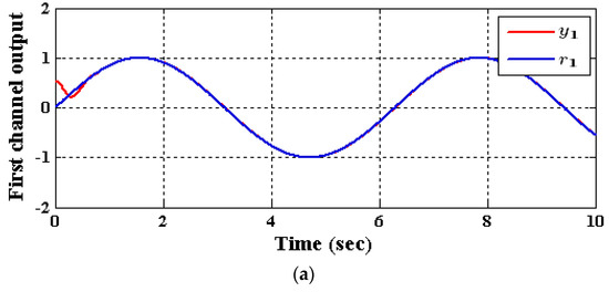
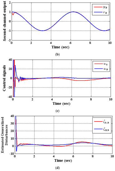
Figure 6.
The output response of Equation (42) using CADRC configuration, (a) output , (b) output , (c) control signals and , and (d) estimated generalized disturbances and [23].
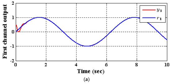
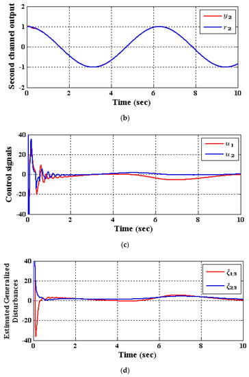
Figure 7.
The output response of Equation (42) using IADRC, (a) output , (b) output , (c) control signals and , and (d) estimated generalized disturbances and [23].
As illustrated in Table 3, the reduction was very evident in the values of the ITAE and ISU indices of the two channels for the second configuration, except for ISU1, where it slightly reduced from its value in the CADRC. This has been reflected in the control efforts and shown in Figure 6c and Figure 7c, where and for the IADRC witnessed less activity than the CADRC. The tracking output response for the IADRC was better than in the CADRC, specifically during the transient period, where both configurations entirely attenuated the effect of the exogenous disturbances and , the state couplings for each subsystem, and the time-varying input gains , , , and on the output response of the two channels.
- Case (2): Input and State Decoupling
Two reference inputs and sequentially applied to the nonlinear system (Equation (42)) to check the disassociation of the input and state couplings between the two subsystems. The transient response of the outputs and in response to reference inputs and are illustrated in Figure 8 and Figure 9. As can be noticed from these figures, the decoupling requirement, stated in the problem statement, was very well satisfied, with a smooth response on each output channel. The proposed scheme converted the nonlinear system of Equation (1) into two non-interacted SISO subsystems.
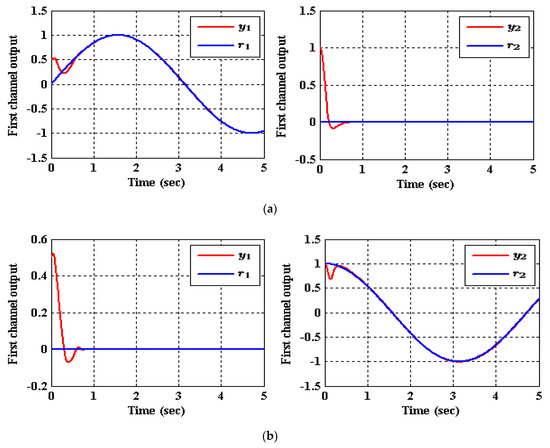
Figure 8.
The output tracking of Equation (42) due to reference inputs and using a decoupled control scheme with CADRC, (a) ; (b) [23].
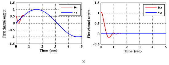
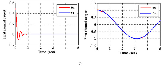
Figure 9.
The output tracking of Equation (42) due to reference inputs and using a decoupled control scheme with IADRC, (a) ; (b) [23].
5.2. Results of the Decentralized ADRC Control Scheme
The proposed decentralized control scheme based on IADRC configuration for the MIMO system in Equation (42) was simulated for tracking the same reference input signalsand as in the simulation of the first scheme. The same two configurations used in the simulations of the decupled control scheme will be utilized here again for comparison purposes with , . Specifically, the proposed control laws and are the saturated values of that in Equation (16), where is given by Equation (26), i.e., they are reformulated as:
where , is a design parameter and is defined as in Equation (50). The parameters of the first and second configuration of the decentralized ADRC scheme for the two channels are listed in Table 4; Table 5, respectively.
Table 4.
The parameters of the first configuration (CADRC).
Table 5.
The parameters of the second configuration (IADRC).
The same scenarios used in the validation of the decoupled control scheme [23] were used here to check the effectiveness of the decentralized control scheme and compare between both schemes.
- Case (1): Output tracking
Two reference signals, and , were applied to the closed-loop system of Figure 5 to authenticate the output tracking capability of the proposed decentralized control scheme, using both CADRC and IADRC configurations. The performance indices for the two configurations are listed in Table 6. For these two configurations, the output response curves of the numerical simulations for the proposed decentralized scheme based on ADRC are shown in Figure 10 and Figure 11, respectively. As illustrated in Table 6, the reduction in the values of the ITAE and ISU indices for the two channels in the IADRC is apparent, in comparison with the CADRC.
Table 6.
Performance of the decentralized ADRC scheme.
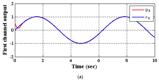
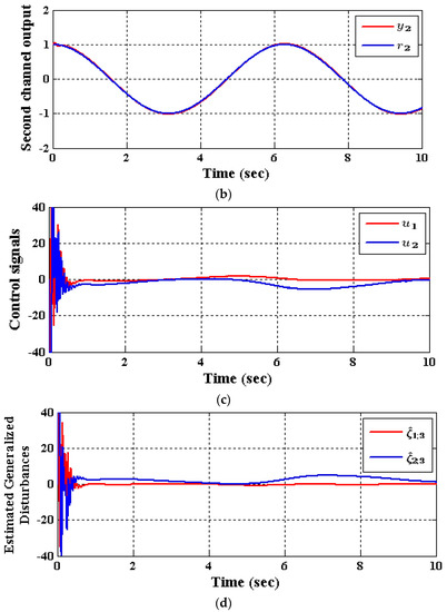
Figure 10.
The output response of Equation (42) using CADRC, (a) output , (b) output , (c) control signals and , and (d) estimated generalized disturbances and .
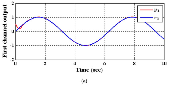
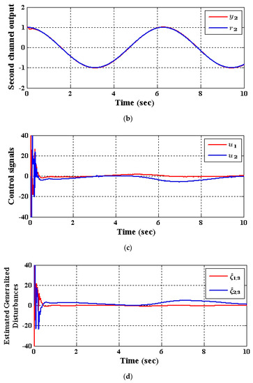
Figure 11.
The output response of (42) using IADRC, (a) output curve , (b) output curve , (c) control signals and , and (d) estimated generalized disturbances and .
Moreover, less chattering control efforts and were produced by the IADRC, in contrast with their counterparts in the first configuration. The tracking output response for the IADRC was better than in the CADRC, specifically during the transient period, where both configurations entirely attenuated the effect of the exogenous disturbances and, the state couplings for each subsystem, and the time-varying input gains , , , and on the output response of the two channels. It should be noted that the exogenous disturbances and are taken as , which simulate a big mismatch between the nominal process and the mathematical model upon all the closed-loop simulations that have been demonstrated. The nominal model is represented by the following mathematical model with the functions and without the external disturbances and , as shown below:
where and are defined during the simulations, as: Now, and are time-varying, which forces and to be time-varying, too. Moreover, it was mentioned previously that the coefficient is approximate of in the system with a ±50% zone, where, during the simulations, we took the worse-case condition for the coefficients , , , , i.e., they are considered as time-varying coefficients with, and . This reflects a big mismatch between the nominal process, where no external disturbances are acting on it and it has no parameter variation, and the mathematical model used in the simulations with external disturbances and inherent parameter uncertainties.
- Case (2): Input and State Decoupling
Two reference inputs and sequentially applied to the nonlinear system (Equation (42)) to check the disassociation of the input and state couplings between the two subsystems. The transient response of the outputs and , in response to reference inputs and sequentially applied to the nonlinear system of Equation (42), are shown in Figure 12 and Figure 13. As can be seen from these figures, the decoupling requirement stated in the problem statement was very well satisfied, with a smooth response on each output channel. The proposed decentralized control scheme converted the nonlinear system of Equation (1) into two non-interacted SISO subsystems.
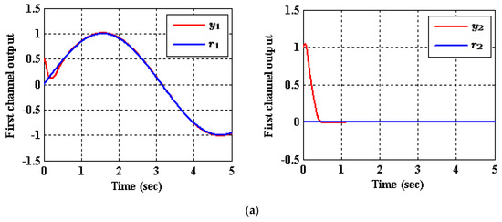
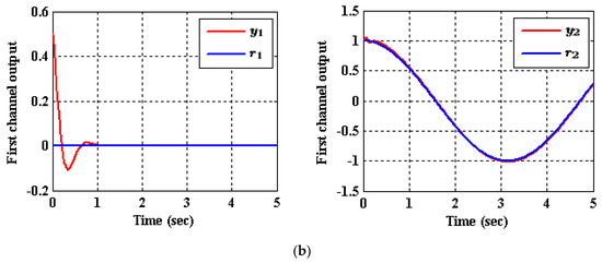
Figure 12.
The output tracking of Equation (42) due to reference inputs and using decentralized control scheme with CADRC, (a) , (b) .
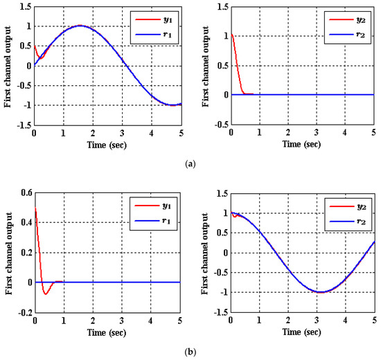
Figure 13.
The output tracking of (42) due to reference inputs and , using a decentralized control scheme with IADRC, (a) ; (b) .
5.3. Comparison between the Proposed Decentralized Scheme and the Decoupled Control [23]
For controlling nonlinear MIMO systems, the nonlinear couplings between different subsystems were considered as the most significant difficulty. Therefore, it was necessary to adopt a control technique that was both simple and robust. A control scheme was suggested in this paper, which makes use of the IADRC because of its robustness and model-independent features. The nonlinear coupling, along with other uncertainties, were considered as a part of the generalized disturbances that needed to be estimated and rejected using the ADRC configuration.
In the decoupled ADRC scheme [23], the decoupling process was accomplished through the decoupler unit, where the control input for each channel was composed by gathering several control signals from each ADRC controller. For this reason, the energy consumed by each input was larger than the energy consumed in the decentralized ADRC scheme, in which the controlled system was decomposed into several SISO subsystems and an ADRC controller was responsible for controlling each SISO subsystem individually. The chattering in the control signals in the decoupled ADRC scheme using IADRC lasted for a shorter amount of time than in the case of CADRC, because the proposed NHOESO needed more time for its output to become settled. The decentralized control scheme achieved a significant control energy reduction, as compared to the decoupled control scheme; this is evident from Table 7, shown below.
Table 7.
Total control energy (ISU1+ISU2).
In the decentralized ADRC scheme, given that the generalized disturbances will have more terms to be rejected, for instance, unwanted control inputs, exogenous disturbances, undesirable dynamics, uncertainties, etc., the accuracy of the decentralized ADRC scheme, as compared to the decoupling ADRC scheme, was reduced further. This reduction was apparent in the differences between the ITAE values of Table 3; Table 6 and Figure 10c,d and Figure 11c,d, where large chattering was seen in the control signals and the generalized disturbances at the very start of the simulation time and vanished quickly due to the reasons mentioned earlier.
Finally, looking back at Figure 8, Figure 9, and Figure 12 and Equation (13), the diagonalization in the output response in both schemes was due to the off-diagonal terms cancellation (input cross-couplings) of the nonlinear system, using the -matrix in the decoupled ADRC scheme [23] and considering other inputs from different channels as unwanted dynamics to be cancelled within the generalized disturbance in the decentralized ADRC scheme. The other reason for the diagonal output response was because of the state couplings cancellation between different individual channels within the ADRC framework inside each proposed scheme.
6. Conclusions
In this paper, the ADRC paradigm was utilized for controlling nonlinear MIMO systems. The suggested decentralized control scheme used the IADRC due to its aforementioned supreme features. The investigation into the MIMO systems indicated potential issues relating to the computing of the input gain matrix. Consequently, the decentralized control scheme based on IADRC configuration had a higher chance than the decoupled ADRC of Reference [23], to be applied practically due to its simplicity in considering inputs from other channels as part of the generalized disturbance; hence, it saved more control energy than the decoupled control scheme, as argued through the simulations (the reduction was 20.8% using CADRC and 27.18% using IADRC). Finally, it can be concluded that the performance of the IADRC in both schemes is significantly higher than its counterpart of the CADRC regarding output tracking, control energy, and chattering, where the reduction in the ITAE index in the decentralized control scheme was 20.8% and 28.5% for the 1st and 2nd channels, respectively, while the reduction was 25.7% and 73.5% for the 1st and 2nd channels, respectively, using the decoupled control scheme. Future extension to the current work might include applying the proposed control decentralized control scheme on a real MIMO platform, such as the twin rotor aerodynamic system (TRAS).
Author Contributions
Conceptualization, I.K.I. and W.R.A.-A.; methodology, I.K.I, W.R.A.-A., A.T.A, and A.J.H.; software, W.R.A.-A. and A.J.H.; validation, A.T.A. and A.J.H; formal analysis, I.K.I., W.R.A.-A., A.T.A., and A.J.H; resources, A.J.H., A.T.A.; writing—original draft preparation W.R.A.-A., I.K.I.; writing—review and editing, W.R.A.-A., I.K.I., A.T.A., and A.J.H, A.T.A.; visualization, I.K.I. and W.R.A.-A.; funding acquisition, A.T.A. All authors have read and agreed to the published version of the manuscript.
Funding
This research is funded by Prince Sultan University, Riyadh, Kingdom of Saudi Arabia. Special acknowledgement to Robotics and Internet-of-Things Lab (RIOTU), Prince Sultan University, Riyadh, Saudi Arabia. We would like to show our gratitude to Prince Sultan University, Riyadh, Saudi Arabia.
Conflicts of Interest
The authors declare no conflict of interest.
References
- Han, J. A Class of Extended State Observers for Uncertain Systems. Control Decis. 1995, 10, 85–88. [Google Scholar]
- Gao, Z. Scaling and bandwidth-parameterization based controller tuning. In Proceedings of the American Control Conference, Denver, CO, USA, 4–6 June 2003; pp. 4989–4996. [Google Scholar] [CrossRef]
- Humaidi, A.J.; Ibraheem, I.K. Speed Control of Permanent Magnet DC Motor with Friction and Measurement Noise Using Novel Nonlinear Extended State Observer-Based Anti-Disturbance Control. Energies 2019, 12, 1651. [Google Scholar] [CrossRef]
- Ibraheem, I.K.; Abdul-Adheem, W.R. A Novel Second-Order Nonlinear Differentiator with Application to Active Disturbance Rejection Control. In Proceedings of the 1st International Scientific Conference of Engineering Sciences—3rd Scientific Conference of Engineering Science (ISCES), Diyalah, Iraq, 10–11 January 2018; pp. 68–73. [Google Scholar] [CrossRef]
- Ibraheem, I.K.; Abdul-Adheem, W.R. An Improved Active Disturbance Rejection Control for a Differential Drive Mobile Robot with Mismatched Disturbances and Uncertainties. arXiv 2018, arXiv:1805.12170. [Google Scholar]
- Chen, Z.; Wang, Y.; Sun, M.; Sun, Q. Convergence and stability analysis of active disturbance rejection control for first-order nonlinear dynamic systems. Trans. Inst. Meas. Control 2019, 41, 2064–2076. [Google Scholar] [CrossRef]
- Cheng, Y.; Chen, Z.; Sun, M.; Sun, Q. Cascade Active Disturbance Rejection Control of a High-Purity Distillation Column with Measurement Noise. Ind. Eng. Chem. Res. 2018, 57, 4623–4631. [Google Scholar] [CrossRef]
- Hou, Y.; Gao, Z.; Jiang, F.; Boulter, B.T. Active Disturbance Rejection Control for Web Tension Regulation. In Proceedings of the 40th IEEE Conference on Decision and Control, Orlando, FL, USA, 4–7 December 2001; pp. 4974–4979. [Google Scholar] [CrossRef]
- Su, Y.X.; Zheng, C.H.; Sun, D.; Duan, B.Y. A simple nonlinear velocity estimator for high-performance motion control. IEEE Trans. Ind. Electron. 2005, 52, 1161–1169. [Google Scholar] [CrossRef]
- Sun, B.; Gao, Z. A DSP-Based Active Disturbance Rejection Control Design for a 1-kW H-Bridge DC-DC Power Converter. IEEE Trans. Ind. Electron. 2005, 52, 1271–1277. [Google Scholar] [CrossRef]
- Zheng, Q.; Chen, Z.; Gao, Z. A Dynamic Decoupling Control Approach and Its Applications to Chemical Processes. In Proceedings of the American Control Conference, New York, NY, USA, 11–13 July 2007; pp. 5176–5181. [Google Scholar] [CrossRef]
- Zheng, Q.; Dong, L.; Gao, Z. Control and rotation rate estimation of vibrational MEMS gyroscopes. In Proceedings of the International Conference on Control Applications, Singapore, 1–3 October 2007; pp. 118–123. [Google Scholar] [CrossRef]
- Goforth, F.J.; Gao, Z. An Active Disturbance Rejection Control Solution for Hysteresis Compensation. In Proceedings of the American Control Conference, Seattle, WA, USA, 11–13 June 2008; pp. 2202–2208. [Google Scholar] [CrossRef]
- Yan, B.; Tian, Z.; Shi, S.; Weng, Z. Fault diagnosis for a class of nonlinear systems via ESO. ISA Trans. 2008, 47, 386–394. [Google Scholar] [CrossRef]
- Wu, D.; Chen, K. Design and analysis of precision active disturbance rejection control for noncircular turning process. IEEE Trans. Ind. Electron. 2009, 56, 2746–2753. [Google Scholar] [CrossRef]
- Li, S.; Yang, X.; Yang, D. Active disturbance rejection control for high pointing accuracy and rotation speed. Automatica 2009, 45, 1854–1860. [Google Scholar] [CrossRef]
- Sira-Ramirez, H.; Lopez-Uribe, C.; Velasco-Villa, M. Linear observer-based active disturbance rejection control of the omnidirectional mobile robot. Asian J. Control 2013, 15, 51–63. [Google Scholar] [CrossRef]
- Leonard, F.; Martini, A.; Abba, G. Robust nonlinear controls of model-scale helicopters under lateral and vertical wind gusts. IEEE Trans. Control Syst. Technol. 2012, 20, 154–163. [Google Scholar] [CrossRef]
- Madoński, R.; Kordasz, M.; Sauer, P. Application of a disturbance-rejection controller for robotic-enhanced limb rehabilitation trainings. ISA Trans. 2014, 53, 899–908. [Google Scholar] [CrossRef] [PubMed]
- Texas Instruments. Technical Reference Manual for TMS320F28069M, TMS320F28068M InstaSPIN-MOTION Software; Texas Instruments: Dallas, TX, USA, 2014; pp. 1–57. [Google Scholar]
- Zheng, Q.; Gao, Z. On Practical Applications of Active Disturbance Rejection Control. In Proceedings of the 29th Chinese Control Conference, Beijing, China, 29–31 July 2010; pp. 6095–6100. [Google Scholar]
- Yi, H.; Wenchao, X.U.E.; Gao, Z.; Sira-ramirez, H.; Dan, W.; Mingwei, S. Active Disturbance Rejection Control: Methodology, Practice and Analysis. In Proceedings of the 33rd Chinese Control Conference, Nanjing, China, 28–30 July 2014; pp. 1–5. [Google Scholar] [CrossRef]
- Abdul-adheem, W.R.; Ibraheem, I.K. Decoupled control scheme for output tracking of a general industrial nonlinear MIMO system using improved active disturbance rejection scheme. Alex. Eng. J. 2019, 58, 1145–1156. [Google Scholar] [CrossRef]
- Elmali, H.; Olgac, N. Robust output tracking control of nonlinear MIMO systems via sliding mode technique. Automatica 1992, 28, 145–151. [Google Scholar] [CrossRef]
- Costa, R.R.; Hsu, L.; Imai, A.K.; Kokotovic, P. Lyapunov-based adaptive control of MIMO systems. Automatica 2003, 39, 1251–1257. [Google Scholar] [CrossRef]
- Liu, X.; Jutan, A.; Rohani, S. Almost disturbance decoupling of MIMO nonlinear systems and application to chemical processes. Automatica 2004, 40, 465–471. [Google Scholar] [CrossRef]
- Bagni, G.; Basso, M.; Genesio, R.; Tesi, A. Synthesis of MIMO controllers for extending the stability range of periodic solutions in forced nonlinear systems. Automatica 2005, 41, 645–654. [Google Scholar] [CrossRef]
- Mizumoto, I.; Chen, T.; Ohdaira, S.; Kumon, M.; Iwai, Z. Adaptive output feedback control of general MIMO systems using multirate sampling and its application to a cart—Crane system. Automatica 2007, 43, 2077–2085. [Google Scholar] [CrossRef]
- Gündes, A.N.; Mete, A.N.; Palazoglu, A. Reliable decentralized PID controller synthesis for two-channel MIMO processes. Automatica 2009, 45, 353–363. [Google Scholar] [CrossRef]
- Chen, M.; Ge, S.S.; Ren, B. Adaptive tracking control of uncertain MIMO nonlinear systems with input constraints. Automatica 2011, 47, 452–465. [Google Scholar] [CrossRef]
- Chiu, C.S. Derivative and integral terminal sliding mode control for a class of MIMO nonlinear systems. Automatica 2012, 48, 316–326. [Google Scholar] [CrossRef]
- Lu, L.; Yao, B. Online constrained optimization based adaptive robust control of a class of MIMO nonlinear systems with matched uncertainties and input/state constraints. Automatica 2014, 50, 864–873. [Google Scholar] [CrossRef]
- Hashemi, M.; Ghaisari, J.; Askari, J. Adaptive control for a class of MIMO nonlinear time delay systems against time varying actuator failures. ISA Trans. 2015, 57, 23–42. [Google Scholar] [CrossRef] [PubMed]
- Zhu, J.; Yu, X.; Zhang, T.; Cao, Z.; Yang, Y.; Yi, Y. Sliding mode control of MIMO Markovian jump systems. Automatica 2016, 68, 286–293. [Google Scholar] [CrossRef]
- Pandey, V.K.; Kar, I.; Mahanta, C. Controller design for a class of nonlinear MIMO coupled system using multiple models and second level adaptation. ISA Trans. 2017, 69, 256–272. [Google Scholar] [CrossRef]
- Wang, L.; Isidori, A.; Liu, Z.; Su, H. Robust output regulation for invertible nonlinear MIMO systems. Automatica 2017, 82, 278–286. [Google Scholar] [CrossRef]
- Feng, Y.; Zhou, M.; Zheng, X.; Han, F.; Yu, X. Full-order terminal sliding-mode control of MIMO systems with unmatched uncertainties. J. Frankl. Inst. 2018, 355, 653–674. [Google Scholar] [CrossRef]
- Zhao, K.; Song, Y.; Zhang, Z. Tracking control of MIMO nonlinear systems under full state constraints: A Single-parameter adaptation approach free from feasibility conditions. Automatica 2019, 107, 52–60. [Google Scholar] [CrossRef]
- Li, J.; Du, J. Adaptive disturbance cancellation for a class of MIMO nonlinear Euler–Lagrange systems under input saturation. ISA Trans. 2020, 96, 14–23. [Google Scholar] [CrossRef]
- Chen, M.; Mei, R.; Jiang, B. Sliding mode control for a class of uncertain MIMO nonlinear systems with application to near-space vehicles. Math. Probl. Eng. 2013, 2013, 180589. [Google Scholar] [CrossRef]
- Chen, M.; Shi, P.; Lim, C.C. Robust Constrained Control for MIMO Nonlinear Systems Based on Disturbance Observer. IEEE Trans. Automat. Contr. 2015, 60, 3281–3286. [Google Scholar] [CrossRef]
- Floquet, T.; Spurgeon, S.K.; Edwards, C. An output feedback sliding mode control strategy for MIMO systems of arbitrary relative degree. Int. J. Robust Nonlinear Control 2011, 21, 119–133. [Google Scholar] [CrossRef]
- Polyakov, A.; Efimov, D.; Perruquetti, W. Sliding Mode Control Design for MIMO Systems: Implicit Lyapunov Function Approach. In Proceedings of the 2014 European Control Conference (ECC), Strasbourg, France, 24–27 June 2014; pp. 2612–2617. [Google Scholar] [CrossRef]
- Ibraheem, I.K. Anti-Disturbance Compensator Design for Unmanned Aerial Vehicle. J. Eng. 2020, 26, 86–103. [Google Scholar] [CrossRef][Green Version]
- Khalil, H.K. Extended High-Gain Observers as Disturbance Estimators. SICE J. Control. Meas. Syst. Integr. 2017, 10, 125–134. [Google Scholar] [CrossRef]
- Tong Shaocheng, T.; Bin, C.; Yongfu, W. Fuzzy adaptive output feedback control for MIMO nonlinear systems. Fuzzy Sets Syst. 2005, 156, 285–299. [Google Scholar] [CrossRef]
- Kim, E.; Lee, S. Output feedback tracking control of MIMO systems using a fuzzy disturbance observer and its application to the speed control of a PM synchronous motor. IEEE Trans. Fuzzy Syst. 2005, 13, 725–741. [Google Scholar]
- Zhang, T.P.; Yang, Y.I. Adaptive Fuzzy Control for a Class of MIMO Nonlinear Systems with Unknown Dead-zones. Acta Autom. Sin. 2007, 33, 96–99. [Google Scholar] [CrossRef]
- Chen, C.H.; Lin, C.M.; Chen, T.Y. Intelligent adaptive control for MIMO uncertain nonlinear systems. Expert Syst. Appl. 2008, 35, 865–877. [Google Scholar] [CrossRef]
- Yousef, H.; Hamdy, M.; El-Madbouly, E.; Eteim, D. Adaptive fuzzy decentralized control for interconnected MIMO nonlinear subsystems. Automatica 2009, 45, 456–462. [Google Scholar] [CrossRef]
- Liu, Y.J.; Tong, S.C.; Li, T.S. Observer-based adaptive fuzzy tracking control for a class of uncertain nonlinear MIMO systems. Fuzzy Sets Syst. 2011, 164, 25–44. [Google Scholar] [CrossRef]
- Li, T.; Li, R.; Wang, D. Adaptive neural control of nonlinear MIMO systems with unknown time delays. Neurocomputing 2012, 78, 83–88. [Google Scholar] [CrossRef]
- Li, C.; Wang, W. Fuzzy almost disturbance decoupling for MIMO nonlinear uncertain systems based on high-gain observer. Neurocomputing 2013, 111, 104–114. [Google Scholar] [CrossRef]
- Zhen, H.T.; Qi, X.H.; Li, J.; Tian, Q.M. Neural network L1 Adaptive control of MIMO systems with nonlinear uncertainty. Sci. World J. 2014, 2014, 1–8. [Google Scholar] [CrossRef]
- Rong, H.J.; Wei, J.T.; Bai, J.M.; Zhao, G.S.; Liang, Y.Q. Adaptive neural control for a class of MIMO nonlinear systems with extreme learning machine. Neurocomputing 2015, 149, 405–414. [Google Scholar] [CrossRef]
- Yan, P.; Liu, D.; Wang, D.; Ma, H. Data-driven controller design for general MIMO nonlinear systems via virtual reference feedback tuning and neural networks. Neurocomputing 2016, 171, 815–825. [Google Scholar] [CrossRef]
- Shi, W. Observer-based adaptive fuzzy prescribed performance control for feedback linearizable MIMO nonlinear systems with unknown control direction. Neurocomputing 2019, 368, 99–113. [Google Scholar] [CrossRef]
- Huo, X.; Ma, L.; Zhao, X.; Zong, G. Event-triggered adaptive fuzzy output feedback control of MIMO switched nonlinear systems with average dwell time. Appl. Math. Comput. 2020, 365, 124665. [Google Scholar] [CrossRef]
- Wang, L.Y.; Zhang, J.F. Fundamental Limitations and Differences of Robust and Adaptive Control. In Proceedings of the 2001 American Control Conference, Arlington, VA, USA, 25–27 June 2001; pp. 4802–4807. [Google Scholar]
- Hespanha, J.P.; Liberzon, D.; Morse, A.S. Overcoming the limitations of adaptive control by means of logic-based switching. Syst. Control Lett. 2003, 49, 49–65. [Google Scholar] [CrossRef]
- Mandoski, R. On Active Disturbance Rejection in Robotic Motion Control. Ph.D. Thesis, University of Poznan, Poznań, Poland, 2016. [Google Scholar] [CrossRef]
- Han, J. From PID to active disturbance rejection control. IEEE Trans. Ind. Electron. 2009, 56, 900–906. [Google Scholar] [CrossRef]
- Abdul-adheem, W.R.; Ibraheem, I.K. Improved Sliding Mode Nonlinear Extended State Observer based Active Disturbance Rejection Control for Uncertain Systems with Unknown Total Disturbance. Int. J. Adv. Comput. Sci. Appl. 2016, 7, 80–93. [Google Scholar] [CrossRef]
© 2020 by the authors. Licensee MDPI, Basel, Switzerland. This article is an open access article distributed under the terms and conditions of the Creative Commons Attribution (CC BY) license (http://creativecommons.org/licenses/by/4.0/).