Abstract
A dashboard application is proposed and developed to act as a Digital Twin that would indicate the Measured Value to be held accountable for any future failures. The current study describes a method for the exploitation of historical data that are related to production performance and aggregated from IoT, to eliciting the future behavior of the production, while indicating the measured values that are responsible for negative production performance, without training. The dashboard is implemented in the Java programming language, while information is stored into a Database that is aggregated by an Online Analytical Processing (OLAP) server. This achieves easy Key Performance Indicators (KPIs) visualization through the dashboard. Finally, indicative cases of a simulated transfer line are presented and numerical examples are given for validation and demonstration purposes. The need for human intervention is pointed out.
1. Introduction
Todays’ manufacturing era focuses on monitoring the process on shop-floor by utilizing various sensorial systems that are based on data collection [1,2,3]. The automated systems directly collect an enormous amount of performance data from the shop-floor (Figure 1), and are stored into a repository, in a raw or accumulated form [4,5]. However, automated decision making in the era of Industry 4.0 is yet to be discovered. The current work is a step towards holistic alarms management (independently of context [6]), and, in particular, automated root-cause analysis.
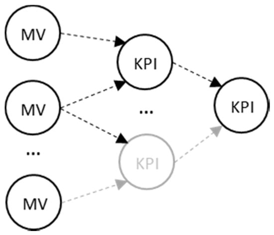
Figure 1.
Key Performance Indications (KPIs) aggregation from Measured Values (MV).
1.1. KPIs and Digital Twin Platforms in Manufacturing
A lot of KPIs have been defined in literature (Manufacturing, Environmental, Design, and Customer) [7], and, despite the fact that methods have been developed for the precise acquisition of measured values [8], the interconnection of the values (Figure 1) can lead to mistaken decision making when one searches for the root cause of an alarm occurring in a manufacturing environment.
In addition, regarding manufacturing-oriented dashboard systems, they aid in the visualization of complex accumulations, trends, and directions of Key Performance Indications (KPIs) [9]. However, despite the situation awareness [10] that they offer, they are not able to support the right decision made at management level by elaborating automatically the performance metrics and achieving profitable production [11]. In the meantime, multiple criteria methods are widely used for decision support or the optimization of production, plant, or machine levels [1,12], based (mainly) on the four basic manufacturing attributes i.e.,: Cost, Time, Quality, and Flexibility levels [1]. This set of course can be extended. The “performance” that is collected from the shop-floor has been considered as measured values (MV) and their aggregation or accumulation into higher level Key Performance Indicators, as initially introduced by [13]. The goal of all these is the achievement of digital manufacturing [14].
On the other hand, the term digital twin can be considered as an “umbrella”, and it can be implemented with various technologies beneath, such as physics [15], machine learning [16], and data/control models [17]. A digital twin deals with giving some sort of feedback back to the system and it varies from process level [15] to system level [18], and it can even handle design aspects [19].
Regarding commercial dashboard solutions, they enable either manual or automated input of measured values for the production of KPIs [20,21,22]. However, their functionality is limited to the reporting features of the current KPI values, typically visualized with a Graphical User Interface (GUI), usually cluttered, with gauges, charts, or tabular percentages. Additionally, there is need to incorporate various techniques from machine learning or Artificial Intelligence in general [23] and signal processing techniques [24]. The typical functionality that is found in dashboards serves as a visual display of the most important information for one or more objectives, consolidated and arranged on a single screen, so as for the information to be monitored at a glance [9]. This is extended in order to analyze the aggregated KPIs and explore potential failures in the future by utilizing monitored production performances. Finding, however, the root cause of a problem occurring, utilizing the real time data in an efficient and fast way, is still being pursued.
1.2. Similar Methods and Constrains on Applicability
In general, categories in root-cause finding are hard to be defined, but if one borrows the terminology from Intrusion Detection Alarms [25], they can claim that there are three major categories: anomaly detection, correlation, and clustering. Specific examples of all three in decision making are given below, in the next paragraph. The alternative classifications of the Decision Support Systems that are given below permit this categorization; the first classification [26] regards: (i) Industry specific packages, (ii) Statistical or numerical algorithms, (iii) Workflow Applications, (iv) Enterprise systems, (v) Intelligence, (vi) Design, (vii) Choice, and (viii) Review. Using another criterion, the second classification [27] concerns: (a) communications driven, (b) data driven, (c) document driven, (d) knowledge driven, and (e) model driven.
There are several general purpose methods that are relevant and are mentioned here to achieve root-cause finding. Root Cause Analysis is a quite good set of techniques, however, it remains on the descriptive empirical strategy level [28,29]. Moreover, scorecards are quite descriptive and empirical, while the Analytical Hierarchical Process (AHP) requires criteria definition [30]. Finally, Factor Analysis, requires a specific kind of manipulation/modelling due to its stochastic character [31].
Regarding specific applications in manufacturing-related decision making, usually finding that the root-cause has to be addressed through identifying a defect in the production. Defects can refer to either product unwanted characteristics, or resources’ unwanted behaviour. Methods that have been previously used—regardless of the application—are Case Based Reasoning [32], pattern recognition [33,34], Analysis of Variance (ANOVA) [35], neural networks [36], Hypothesis testing [37], Time Series [38], and many others. However, none of these methods is quick enough to give the results from a deterministic point of view and without using previous measurements for training. Additionally, they are quite focused in application terms, which means that they cannot be used without re-calibration to a different set of KPIs. On the other hand, traditional Statistical Process Control (SPC) does not offer solutions without context, meaning the combination of the application and method [31].
1.3. Research Gaps & Novelty
In this work, an analysis method on KPIs has been implemented in the developed dashboard to identify, automatically and without prior knowledge, for a given KPI, the variables that are responsible for an undesired production performance. This mechanism is triggered by predicting a threshold exceedance in management level KPIs. The prediction utilizes (linear) regression, which is applied on the historical trend of each variable for the estimation of the performance values for the upcoming working period in order for the weaknesses of the production to be elicited beforehand. The dashboard in which the current methodology has been framed acts as an abstractive Digital Twin for production managers and it supports automated decision making.
In the following sections, the analysis approach is presented, followed by its implementation details within dashboard. The results from case studies, the points of importance, and the future research trends have been discussed.
2. Materials and Methods
2.1. The Description of the Flow and the Calculations
The current method consists of two stages. Initially, the formulas of each KPI are analyzed and their dependent variables are collected. Thus, the relationships between the Measured Values (MV), Intermediate Values (IV), Performance Indicators (PI), and Key Performance Indicators (KPIs) are known. This stage, in reality, constitutes the modelling of the production and it runs only once, while the data are aggregated form IoT technologies. The exact methodology can be found as IoT-Production in previous literature [39]. Regarding the second stage, Figure 2 presents its flow of the analysis for a single KPI. This stage runs continuously. In the beginning, the trend for each measure of the current period that is examined is acquired from the OLAP. For reasons of flexibility and modularity, they are not directly acquired from the data acquisition system. The measure trend is supplied as input to the tool, whereas a linear regression is applied to the estimation of the data points until the end of the next period, namely, horizon (as defined in detail of Figure 3). Once an estimated value is over the measure of the supposed goal (A1/A2), it is marked as ‘out-of-goal’ and the user is notified by the user interface. The user can then choose to repeat the process for lower level KPIs (turning it into investigated metric), after the automated suggestion of the analysis tool as to who is accounted for this result (B). The analysis method utilizes differentials; this mathematical approach that utilizes differentials is explained hereafter. The decisions that have to be taken (C) are beyond the scope of the current work. Nevertheless, it is noted that their generation often is straightforward, even though the existence of a knowledge base, to this end, would be extremely useful.
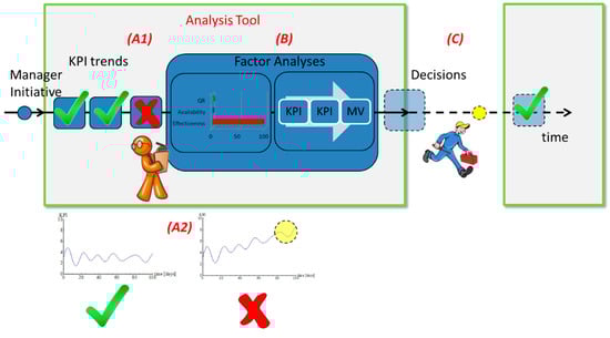
Figure 2.
Schematic of the way the tool is run in real production.
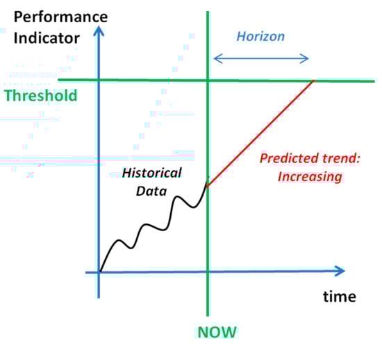
Figure 3.
Alarm that is created by prediction of KPI exceeding threshold.
Figure 4 summarizes this procedure while using a flowchart. Additionally, for easy comprehension, the algorithmic description follows, along with some notes for each step.
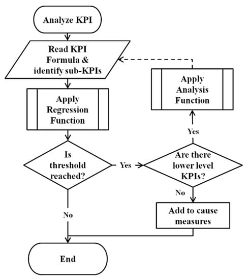
Figure 4.
Flow chart of the algorithmic procedure.
- All of the KPIs are checked for alarms (exceedance of specific value in the future) through regression. This KPI can be named an “investigated metric”.KPIs historical values are retrieved with OLAP Queries. In continuation, (Linear) Extrapolation is used to predict the tendency and trigger alarms. To this end, thresholds and time horizons, as per Figure 3, have to be defined prior to running the tool, and their definition has been made via the production characteristics; for instance, in the case of monetary metrics, the desired profit is the criterion. In other cases, such as quality, tolerances are the basis for this definition.
- If an investigated metric is found to create an alarm, all of its constituent PIs are evaluated in terms of contribution.This step is the Key Concept to the current algorithm and it is quite easy to run, as the relationship between the metrics is already known. Although, the exact relationship is required; in case only the constituents are known, the method cannot be applied. Additionally, the method used here is computationally light, as the relations are pure algebraic. At the time of the creation of the tool, the hierarchy of the indicators has been documented in a database-like structure, where information about the path is logged, including the operations. In the context of a specific example, it is mentioned that Figure 5 is indicative of the graphical illustration of such information. The derivatives formulas are also pre-installed, as they are used during this step.
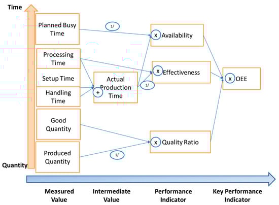 Figure 5. Relationship between Measured Values and KPI. Operations include summation, products and inversion.
The partial differential is the tool that is applied within the analysis function used to estimate the cause of the variation. It is a powerful tool that deterministically quantifies the effect of the variation of one KPI to the variation of another KPI. More specifically, if KPI A(t) is a function of PIs A1(t), A2(t), and A3(t), the percentage that each An(t) contributes in the variation of A(t) in time is the quantity
Given the corresponding notation, the operators of absolute value |·|, mean value ℇ{·}, partial derivative ∂/∂X, and difference Δ are used for the computation of the mean partial differential. This helps in pointing out the direction that the production manager should focus on.
- The constituent PI(s) that are found to cause this variation are turned into “investigated metric(s)” and #2 is run again. Its constituents KPIs are checked. Unless the investigated PIs are Measured Values, the loop continues.The operator can stop this loop at will at any level. However, in most cases, it is the Measured Value, which gives the maximum of information regarding the actions that have to be taken, as PIs of higher level depend on a variety of factors (the final case study is an appropriate case).
- The MV(s) that has come up during the procedure is considered to be the root cause of the alarm.This result has been given without much effort, as in case other methods would have used, more information would be needed; SPC would require expert operators, AHP would require voting among experts, machine learning, ANOVA, and Hypothesis Testing would require exposure to similar situations and Time Series do not guarantee the optimal use of models.
- Directives are given to the operators for actions through a knowledge base if it is not straight-forward.
2.2. Implementation within a Dashboard: Services and Hardware Framework
The dashboard is implemented in Java in an Object-Oriented (OO) paradigm as a Web Application that runs on a typical Java Servlet Container (Apache Tomcat); thus, it is accessible through a typical Internet browser. The Digital Twin is implemented in a Service-Oriented Architecture (SOA) that follows the N-Tier Architecture with multiple layers per tier. An integration layer handles the asynchronous communication of the browser with the server by enabling the user to begin the analysis at any time and without leaving the current screen. The browser sends HTTP requests to the server, whereas the JavaScript Object Notation (JSON) objects, which contain the results, are returned to the client.
Figure 6 illustrates the system’s architecture comprising two individual processes. The Monitor Process records every equipment performance activity in the database, while the Actor directly interacts with the Analysis Process through the dashboard pages and requests an analysis for certain KPIs. Numbers 1 and 6 are indicative of communication between human (engineer/operator) and the dashboard, 2 and 5 denote a query request or result, and 3 and 4 are indicative of the OLAP/RDBMS communication.
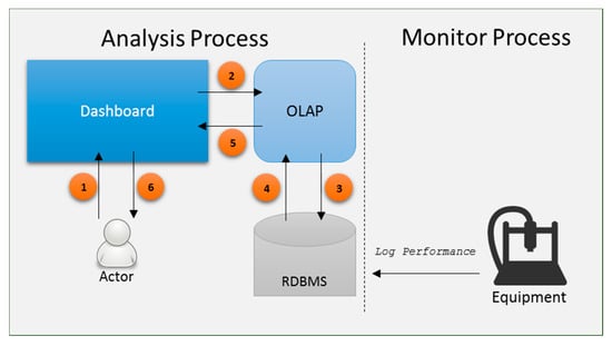
Figure 6.
Application architecture.
In particular, the Actor interacts with the AnalyticAction of the dashboard, as depicted in Figure 7, which, in turn, cooperates with the AnalysisService, employing the Facade Design Pattern [40]. This architecture allows the usability of a software library and provides a context-specific interface launching a set of services without the user being exposed to the complexity of the algorithms beneath. This performed through a variety of entities. Firstly, the AnalysisService directly uses the OLAPQueryService to acquire the values of the KPIs requested, holds them in the KPIManager along with their formula expression stored into the database—this is due to an implementation limitation of the current OLAP servers providing the calculation function for a KPI. Next, the PredictionTool applies the regression function to the data, which are consecutively fed to the FactorAnalysisTool for the analysis of the influence factor on each dependent variable of the KPI. The PredictionTool and the FactorAnalysisTool both correspond the implementations of the extrapolation tool and the tool estimating differentials that are described in the previous section.
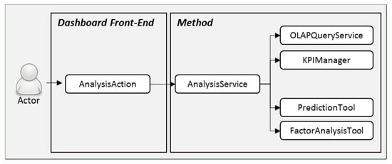
Figure 7.
Unified Model Language (UML) of objects implemented in dashboard and their workflow.
The dashboard also uses the RDBMS to store the information that is required for the visualization of the customized KPI views in various forms. Each KPI is defined in a KPIDefinition instance along with its formula. The Measured Values are retained in the same structure but without a formula. Formulas are lexical names that correspond to definition names. For instance, the Availability KPI is defined by the lower case name ‘availability’, and it is referred to by the OEE KPI as #{availability} variable, whereas the interpreter replaces it at runtime with the actual value. The exact UML of the Informational Model used is given in Figure 8. Black rhombus indicates composition, white rhombus indicates aggregation, and pure arrow indicates association.
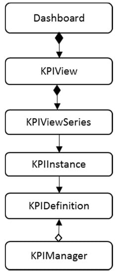
Figure 8.
UML of the Informational Model.
Historical data of the production’s execution are stored into the relational database management system/RDBMS (Figure 6) as records regarding the depiction of the data acquisition method. A relational table holds the machine’s cycle output, whereas each record represents a single machine cycle with attributes that relate to the corresponding entities in the production system. The smallest set of these attributes can be:
- The Part machined at that moment.
- The Process performed.
- The Equipment used in that cycle.
- The Operator of the equipment.
- The Work Order of the part machined.
- For each machine cycle what can be recorded is:
- The actual setup time spent for the preparation of the equipment.
- The actual processing time spent for the part’s machining.
- The pre-processing time prior to machining being started.
- The post-processing time required for the part’s unloading.
These are attributes and records that mostly refer to productivity. Additional attributes, even of different character (i.e., sustainability related, such as energy consumption), can be added. A graph is then formed with involved KPIs, where each KPI is represented by a vertex v and their dependency by an edge e, similar notation to precedence diagrams. The analysis method exploits the data and follows their dependencies until the root measure has been identified (among Measured Values). Finally, that measure is presented to the user as an indication of the type of measure that will negatively affect the performance of production in the near future.
The production performance is loaded from the OLAP cube [41], where the measures are formed with the help of the aggregation functions. For instance, measure ‘Good Quantity’ is aggregated by the count function of the ‘Good Part’ attribute.
3. Results & Discussion
The functionality of the methodology that is presented in the above sections is proved herein utilizing adequately complex cases. Noise is also present in the first three cases, where dummy KPIs have been used, to simulate the short-time variations of the KPIs. These first case studies have been established in order to check the numerical success of the algorithm, where the fourth case study originates from a real industrial problem and its scope is to test the applicability of the digital twin and the validity of the main algorithm in problems set in environments of higher Technology Readiness Level.
3.1. Case I
In this case, the relationship between the KPI B(t) and the PIs A1(t), A2(t), A3(t) is B(t) = A1(t)*A2(t) + A3(t). The evolution of the PIs trends are as follows:
- A1(t) increases in time;
- A2(t) is constant in time; and,
- A3(t) is constant in time.
It is evident from the contribution diagram of Figure 9 that there is success in predicting that the contribution of the first factor should be high. The same happens if A1(t) decreases in time. Despite the noise existence, the algorithm worked to a satisfactory extent, which resulted in characterizing A1(t) as the root-cause of the variation.
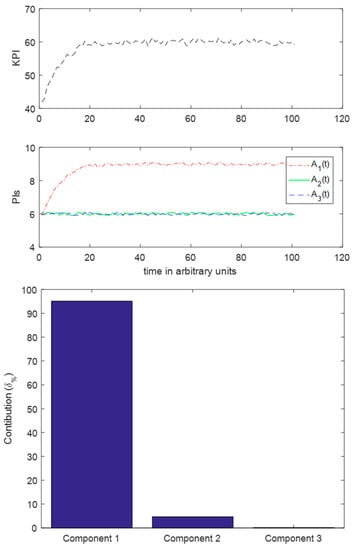
Figure 9.
Case I. Top: Evolution of KPI, Middle: Evolution of PIs, Bottom, Contribution of each PI.
3.2. Case II
In this case, the relationship between the KPI B(t) and the PIs A1(t), A2(t), A3(t) is B(t) = A1(t)*A2(t) + A3(t). The evolution of the PIs trends is, as follows:
- A1(t) is constant in time;
- A2(t) is constant in time; and,
- A3(t) increases in time.
It is evident from the contribution diagram of Figure 10 that there is success in predicting that the contribution of the third factor should be high. The same happens if A3(t) decreases in time. It seems that the algorithm runs successfully, regardless of the operations that are performed among the KPIs.
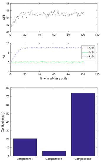
Figure 10.
Case II. Top: Evolution of KPI, Middle: Evolution of PIs, Bottom, Contribution of each PI.
3.3. Case III
In this case, the relationship between the KPI B(t) and the PIs A1(t), A2(t), and A3(t) is B(t) = A2(t) / A1(t) + A3(t). The evolution of the PIs trends is, as follows:
- A1(t) decreases in time;
- A2(t) increases in time; and,
- A3(t) is constant in time.
It is evident from the contribution diagram in Figure 11 that there is success in predicting that the contribution of the first signal should be higher than that of the second one. It is apparent that both of the first two PIs are causes of the variation, however, the denominator change is the one that affects more the result. Accordingly, the algorithm has pointed towards the correct correction.
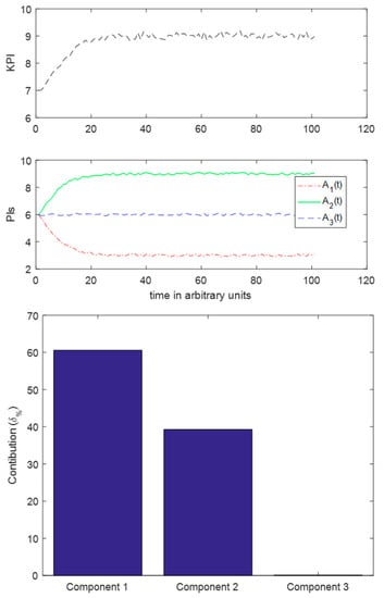
Figure 11.
Case III. Top: Evolution of KPI, Middle: Evolution of PIs, Bottom, Contribution of each PI.
3.4. Case IV
This case regards a true production system and it is used to test the validity of the algorithm in terms of the physical relationship between the PIs. This is done through forcing the Measured Values to create an KPI-level alarm and check whether the algorithm will find the root cause and indicate towards the correct Measured Value. Thus, a production system of thirty (30) identical machines that are arranged in eight work-centers has been simulated by a commercial software [42] (Figure 12). The system simulates a real-life machine-shop producing two variants of Cylinder Head parts: (a) Petrol and (b) Diesel. Different processing times and setup times have been configured. Additionally, negative exponential distribution for Mean-Time-Between-Failures (MTBF), and a real distribution on Mean-Time-To-Repair (MTTR) considered the equipment breakdown on machines. Customer demand has been set by a normal distribution. Finally, the performances have been recorded and manually fed in the informational model.
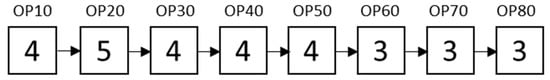
Figure 12.
Workcenters arrangement of the production system. The number indicates the amount of machines for each workcenter.
The KPIs that are utilized in this case study (top to bottom) are mentioned below and their relationship is also given in Figure 5, beginning with Overall Equipment Efficiency (OEE).
- OEE = Availability × Effectiveness × Quality Rate
- Availability = Actual Production Time/Planned Busy Time
- Effectiveness = Processing Time/Actual Production Time
- Quality Ratio = Good Quantity/Produced Quantity
- Actual Production Time = Processing Time + Setup Time + Handling Time
A simulation has been conducted with the machine breakdowns deliberately increased with time. Subsequently, the algorithm of finding the root-cause is run once. In Figure 13, it is clearly shown (yellow shaded rectangles and curved arrows) that the algorithm dictates the major role of Effectiveness. This definitely helps in pointing out the direction that the production manager should focus on.
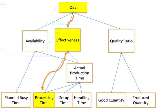
Figure 13.
Tracking the cause of the OEE alarm back to Processing Time.
As a matter of fact, if one repeats the procedure of running the algorithm, but this time utilizing Effectiveness instead of OEE (68% contribution), and then the Measured Value that comes up is Processing Time. This means that the engineer should focus on why the machines do not work that much, which is indeed the root cause of the OEE drop (Figure 13).
It seems that the algorithm works successfully without setting any rules or training. On the contrary, in the literature, works coming up often have to use one or the other, so a direct comparison cannot be made. For instance, in another alarm root cause detection system [43], the authors, even though they are describing the impact on case studies in brief, explicitly point out the need for rules in an internal expert system. Additionally, the use of KPIs at process level [44] is complementary to the current work. A framework that aims to detect the quality of the process, as per classifiers utilizing depth of cut and spindle rate could be integrated; corresponding indicators can be regarded as processed Measured Values. Additionally, the issue of validity of the indicators that are aggregated from IoT is also an issue that has not been raised herein, as the data have been considered to be valid. In addition to this, architectures that are based on complexity handling [45] and algorithms, such as Blockchain [46], can guarantee this goal, while, as indicated by corresponding results in literature [47], the introduction of a manipulation strategy, such as KPI-ML, will boost the performance of any algorithm, including the current. In other pieces of literature [48], the Multiple Alarms Matrix is utilized and hierarchical clustering is applied. In their results, they seem to be presenting the usability of the method towards the correlation of the alarms and extraction of the unique ones. This has not pointed out herein, as the goal has been to search for immediate causal relationships. Inferring Bayesian Networks are utilized in a different work [49]; this approach can also be useful towards a causal model [50]. However, Abele et al., in their own discussion, state the use of probabilities and simulations, while expert knowledge is needed, whereas, in the current work, knowledge use is solely used in the actions generation. Furthermore, the enhancement with Max–Min Hill Climbing algorithm seems to be useful, however it is characterized as time consuming [51]. Case Based Reasoning seems to be similar to the present work, given the results in the literature [52]; however, as per the authors, it is best applied when records of previously successful solutions exist.
Moreover, the environment plays a significant role in the efficiency of such aggregation. More specifically, regarding manufacturing, large networks that share decision making, alternative bandwidth reservation [53] can be adopted for reasons of performance. Connection to control layer, as performed in other works [54], could be potentially addressed in an extension of the current study. Along the same lines, KPIs related to CPPS issues [55] could potentially extend the applicability of the current framework. Finally, regarding innovation and technology readiness, the upscale of technologies that are integrated in shop-floor is also relevant, in terms of decision making for designing systems and process planning integrating Industry 4.0 Key Enabling Technologies. The Technology Readiness Level of the various technologies could also be described in terms of KPIs, as per the literature [56].
4. Conclusions
This paper presents an approach for identifying the measured values that may negatively affect the production performance by eliciting historical data with the aid of Key Performance Indicators. Differentials have been adopted to this effect, being implemented in the developed dashboard and applied to a data set generated by simulation. To achieve this, performances have been stored into an RDBMS system and they have been aggregated through an OLAP server. The key advantage of the method is the quick identification of the root measured value, which will lead the production performance to undesirable directions from the ones expected by the managers, but in a non-supervised way. Therefore, it provides a technique for the development of functional dashboards beyond the visualization of accumulated indicators. Additionally, this paper proposes that dashboard applications, despite being complex and perhaps becoming cluttered up, could be used for automated decision support, as in the case of production performances. The results have shown that managers using the dashboard may be alerted about the weaknesses of their production performance before it is actually done at the shop-floor.
It seems that a digital twin for real time management of production alarms is feasible, and the algebraic notion of differentials is a powerful tool towards this direction. It covers several aspects of a digital twin; it uses the data themselves instead of elaborated models, it is deterministic towards variations (by default), it is immune to noise (at least in the described examples), and, of course, it can be used in loops of automated decision making. However, the use of Human-In-the-Loop Optimization techniques might be inevitable, as the actions derivation, as well as triggering of the tool, may have to include the knowledge that operators have accumulated.
Regarding extensions of the work, knowledge-based libraries for action identification have to be implemented as a continuation to the current approach. Additionally, it seems logical that, besides the mean value, moments of higher order, such as variance, skewness, and kurtosis, could be elaborated to assist decision making. However, the interpretation of these values exceeds the purposes of this study. Another extension is that of the differential order. Derivatives of any order, as well as integrators, could be used to enrich the information that is given to the user. In addition, it has to be mentioned that the definition of the relations between the KPIs is of great importance both to the calculation and to the interpretation of the differentials.
Author Contributions
Conceptualization, P.S. and D.M.; Formal analysis, P.S.; Methodology, A.P.; Software, A.P. and C.G.; Supervision, D.M.; Writing—original draft, A.P. and C.G.; Writing–review & editing, D.M. All authors have read and agreed to the published version of the manuscript.
Funding
This research received no external funding.
Conflicts of Interest
The authors declare no conflict of interest.
References
- Chryssolouris, G. Manufacturing Systems: Theory and Practice; Springer: New York, NY, USA, 2006. [Google Scholar]
- Larreina, J.; Gontarz, A.; Giannoulis, C.; Nguyen, V.K.; Stavropoulos, P.; Sinceri, B. Smart manufacturing execution system (SMES): The possibilities of evaluating the sustainability of a production process. In Proceedings of the 11th Global Conference on Sustainable Manufacturing, Berlin, Germany, 23–25 September 2013; pp. 517–522. [Google Scholar] [CrossRef]
- Ding, K.; Chan, F.T.; Zhang, X.; Zhou, G.; Zhang, F. Defining a digital twin-based cyber-physical production system for autonomous manufacturing in smart shop floors. Int. J. Prod. Res. 2019, 57, 6315–6334. [Google Scholar] [CrossRef]
- Stavropoulos, P.; Chantzis, D.; Doukas, C.; Papacharalampopoulos, A.; Chryssolouris, G. Monitoring and control of manufacturing processes: A review. Procedia CIRP 2013, 8, 421–425. [Google Scholar] [CrossRef]
- Zendoia, J.; Woy, U.; Ridgway, N.; Pajula, T.; Unamuno, G.; Olaizola, A.; Fysikopoulos, A.; Krain, R. A specific method for the life cycle inventory of machine tools and its demonstration with two manufacturing case studies. J. Clean. Prod. 2014, 78, 139–151. [Google Scholar] [CrossRef]
- Al-Kharaz, M.; Ananou, B.; Ouladsine, M.; Combal, M.; Pinaton, J. Evaluation of alarm system performance and management in semiconductor manufacturing. In Proceedings of the 6th International Conference on Control, Decision and Information Technologies (CoDIT), Paris, France, 23–26 April 2019; pp. 1155–1160. [Google Scholar]
- Mourtzis, D.; Fotia, S.; Vlachou, E. PSS design evaluation via kpis and lean design assistance supported by context sensitivity tools. Procedia CIRP 2016, 56, 496–501. [Google Scholar] [CrossRef]
- Peng, K.; Zhang, K.; Dong, J.; Yang, X. A new data-driven process monitoring scheme for key performance indictors with application to hot strip mill process. J. Frankl. Inst. 2014, 351, 4555–4569. [Google Scholar] [CrossRef]
- Few, S. Information Dashboard Design: The Effective Visual Communication of Data; O’Reilly Media, Inc.: Sebastopol, CA, USA, 2006; Volume 3, Edv 161245. [Google Scholar] [CrossRef]
- Ghimire, S.; Luis-Ferreira, F.; Nodehi, T.; Jardim-Goncalves, R. IoT based situational awareness framework for real-time project management. Int. J. Comput. Integr. Manuf. 2016, 30, 74–83. [Google Scholar] [CrossRef]
- Epstein, M.J.; Roy, M.J. Making the business case for sustainability: Linking social and environmental actions to financial performance. J. Corp. Citizsh. 2003, 79–96. [Google Scholar]
- Apostolos, F.; Alexios, P.; Georgios, P.; Panagiotis, S.; George, C. Energy efficiency of manufacturing processes: A critical review. Procedia CIRP 2013, 7, 628–633. [Google Scholar] [CrossRef]
- Kaplan, R.S.; Norton, D.P. The Strategy-Focused Organization: How Balanced Scorecard Companies Thrive in the New Business Environment; Harvard Business School Press: Boston, MA, USA, 2001. [Google Scholar] [CrossRef]
- Mourtzis, D.; Papakostas, N.; Mavrikios, D.; Makris, S.; Alexopoulos, K. The role of simulation in digital manufacturing: Applications and outlook. Int. J. Comput. Integr. Manuf. 2015, 28, 3–24. [Google Scholar] [CrossRef]
- Papacharalampopoulos, A.; Stavropoulos, P.; Petrides, D.; Motsi, K. Towards a digital twin for manufacturing processes: Applicability on laser welding. In Proceedings of the 13th CIRP ICME Conference, Gulf of Naples, Italy, 17–19 July 2019. [Google Scholar]
- Athanasopoulou, L.; Papacharalampopoulos, A.; Stavropoulos, P. Context awareness system in the use phase of a smart mobility platform: A vision system utilizing small number of training examples. In Proceedings of the 13th CIRP Conference on Intelligent Computation in Manufacturing Engineering, Gulf of Naples, Italy, 17–19 July 2019. [Google Scholar]
- Papacharalampopoulos, A.; Stavropoulos, P. Towards a digital twin for thermal processes: Control-centric approach. Procedia CIRP 2019, 86, 110–115. [Google Scholar] [CrossRef]
- Gallego-García, S.; Reschke, J.; García-García, M. Design and simulation of a capacity management model using a digital twin approach based on the viable system model: Case study of an automotive plant. Appl. Sci. 2019, 9, 5567. [Google Scholar] [CrossRef]
- Madni, A.M.; Madni, C.C.; Lucero, S.D. Leveraging digital twin technology in model-based systems engineering. Systems 2019, 7, 7. [Google Scholar] [CrossRef]
- Klipfolio Site 2019. Available online: http://www.klipfolio.com/features#monitor (accessed on 10 February 2020).
- KPI Monitoring 2014. Available online: http://www.360scheduling.com/solutions/kpi-monitoring/ (accessed on 23 October 2016).
- SimpleKPI 2014. Available online: http://www.simplekpi.com/ (accessed on 23 October 2016).
- Monostori, L. AI and machine learning techniques for managing complexity, changes and uncertainties in manufacturing. In Proceedings of the 15th Triennial World Congress, Barcelona, Spain, 21–26 July 2002; pp. 119–130. [Google Scholar] [CrossRef]
- Teti, R. Advanced IT methods of signal processing and decision making for zero defect manufacturing in machining. Procedia CIRP 2015, 28, 3–15. [Google Scholar] [CrossRef]
- Julisch, K. Clustering intrusion detection alarms to support root cause analysis. ACM Trans. Inf. Syst. Secur. 2003, 6, 443–471. [Google Scholar] [CrossRef]
- Sheshasaayee, A.; Jose, R. A theoretical framework for the maintainability model of aspect oriented systems. Procedia Comput. Sci. 2015, 62, 505–512. [Google Scholar] [CrossRef]
- Ada, Ş.; Ghaffarzadeh, M. Decision making based on management information system and decision support system. Eur. Res. 2015, 93, 260–269. [Google Scholar] [CrossRef]
- Energy, U.S.D. Doe Guideline—Root Cause Analysis; US Department of Energy: Washington, DC, USA, 1992; DOE-NE-STD-1004-92.
- Nelms, C.R. The problem with root cause analysis. In Proceedings of the 2007 IEEE 8th Human Factors and Power Plants and HPRCT 13th Annual Meeting, Monterey, CA, USA, 26–31 August 2007; pp. 253–258. [Google Scholar] [CrossRef]
- Kurien, G.P. Performance measurement systems for green supply chains using modified balanced score card and analytical hierarchical process. Sci. Res. Essays 2012, 7, 3149–3161. [Google Scholar] [CrossRef]
- Apley, D.W.; Shi, J. A factor-analysis method for diagnosing variability in mulitvariate manufacturing processes. Technometrics 2001, 43, 84–95. [Google Scholar] [CrossRef]
- Mourtzis, D.; Vlachou, E.; Milas, N.; Dimitrakopoulos, G. Energy consumption estimation for machining processes based on real-time shop floor monitoring via wireless sensor networks. Procedia CIRP 2016, 57, 637–642. [Google Scholar] [CrossRef]
- Masood, I.; Hassan, A. Pattern recognition for bivariate process mean shifts using feature-based artificial neural network. Int. J. Adv. Manuf. Technol. 2013, 66, 1201–1218. [Google Scholar] [CrossRef]
- Stavropoulos, P.; Papacharalampopoulos, A.; Vasiliadis, E.; Chryssolouris, G. Tool wear predictability estimation in milling based on multi-sensorial data. Int. J. Adv. Manuf. Technol. 2016, 82, 509–521. [Google Scholar] [CrossRef]
- Jin, J.; Guo, H. ANOVA method for variance component decomposition and diagnosis in batch manufacturing processes. Int. J. Flex. Manuf. Syst. 2003, 15, 167–186. [Google Scholar] [CrossRef]
- Jeng, J.Y.; Mau, T.F.; Leu, S.M. Prediction of laser butt joint welding parameters using back propagation and learning vector quantization networks. J. Mater. Process. Technol. 2000, 99, 207–218. [Google Scholar] [CrossRef]
- Koufteros, X.A. Testing a model of pull production: A paradigm for manufacturing research using structural equation modeling. J. Oper. Manag. 1999, 17, 467–488. [Google Scholar] [CrossRef]
- Asakura, T.; Ochiai, K. Quality control in manufacturing plants using a factor analysis engine. Nec Tech. J. 2016, 11, 58–62. [Google Scholar]
- Mourtzis, D.; Vlachou, K.; Zogopoulos, V. An IoT-based platform for automated customized shopping in distributed environments. Procedia CIRP 2018, 72, 892–897. [Google Scholar]
- Freeman, E.; Freeman, E. Head First Design Patterns; O’Reilly Media, Inc.: Sebastopol, CA, USA, 2013. [Google Scholar] [CrossRef][Green Version]
- OLAP Server Site 2019. Available online: http://www.iccube.com/ (accessed on 10 February 2020).
- Lanner Witness Site 2020. Available online: https://www.lanner.com/en-us/technology/witness-simulation-software.html (accessed on 10 February 2020).
- Rollo, M.; Novák, P.; Kubalík, J.; Pěchouček, M. Alarm root cause detection system. In Proceedings of the International Conference on Information Technology for Balanced Automation Systems, Vienna, Austria, 27–29 September 2004; pp. 109–116. [Google Scholar]
- Palacios, J.A.; Olvera, D.; Urbikain, G.; Elías-Zúñiga, A.; Martínez-Romero, O.; de Lacalle, L.L.; Rodríguez, C.; Martínez-Alfaro, H. Combination of simulated annealing and pseudo spectral methods for the optimum removal rate in turning operations of nickel-based alloys. Adv. Eng. Softw. 2018, 115, 391–397. [Google Scholar] [CrossRef]
- Lee, J.; Noh, S.D.; Kim, H.J.; Kang, Y.S. Implementation of cyber-physical production systems for quality prediction and operation control in metal casting. Sensors 2018, 18, 1428. [Google Scholar] [CrossRef]
- Fernández-Caramés, T.M.; Blanco-Novoa, O.; Froiz-Míguez, I.; Fraga-Lamas, P. Towards an autonomous industry 4.0 warehouse: A uav and blockchain-based system for inventory and traceability applications in big data-driven supply chain management. Sensors 2019, 19, 2394. [Google Scholar]
- Brandl, D.L.; Brandl, D. KPI Exchanges in smart manufacturing using KPI-ML. IFAC-PapersOnLine 2018, 51, 31–35. [Google Scholar] [CrossRef]
- Chen, Y.; Lee, J. Autonomous mining for alarm correlation patterns based on time-shift similarity clustering in manufacturing system. In Proceedings of the IEEE Conference on Prognostics and Health Management, Denver, CO, USA, 20–23 June 2011; pp. 1–8. [Google Scholar]
- Abele, L.; Anic, M.; Gutmann, T.; Folmer, J.; Kleinsteuber, M.; Vogel-Heuser, B. Combining knowledge modeling and machine learning for alarm root cause analysis. IFAC Proc. Vol. 2013, 46, 1843–1848. [Google Scholar] [CrossRef]
- Büttner, S.; Wunderlich, P.; Heinz, M.; Niggemann, O.; Röcker, C. Managing complexity: Towards intelligent error-handling assistance trough interactive alarm flood reduction. In Proceedings of the International Cross-Domain Conference for Machine Learning and Knowledge Extraction, Reggio, Italy, 29 August–1 September 2017; pp. 69–82. [Google Scholar]
- Wunderlich, P.; Niggemann, O. Structure learning methods for Bayesian networks to reduce alarm floods by identifying the root cause. In Proceedings of the 22nd IEEE International ETFA Conference, Limassol, Cyprus, 12–15 September 2017; pp. 1–8. [Google Scholar]
- Amani, N.; Fathi, M.; Dehghan, M. A case-based reasoning method for alarm filtering and correlation in telecommunication networks. In Proceedings of the Canadian Conference on Electrical and Computer Engineering, Saskatoon, SK, Canada, 1–4 May 2005; pp. 2182–2186. [Google Scholar]
- Zuo, L.; Zhu, M.M.; Wu, C.Q.; Hou, A. Intelligent bandwidth reservation for big data transfer in high-performance networks. In Proceedings of the IEEE International Conference on Communications, Kansas City, MO, USA, 20–24 May 2018; pp. 1–6. [Google Scholar]
- Contuzzi, N.; Massaro, A.; Manfredonia, I.; Galiano, A.; Xhahysa, B. A decision making process model based on a multilevel control platform suitable for industry 4.0. In Proceedings of the 2019 II Workshop on Metrology for Industry 4.0 and IoT, Naples, Italy, 4–6 June 2019; pp. 127–131. [Google Scholar]
- Lüder, A.; Schmidt, N.; Hell, K.; Röpke, H.; Zawisza, J. Description means for information artifacts throughout the life cycle of CPPS. In Multi-Disciplinary Engineering for Cyber-Physical Production Systems; Springer: Berlin/Heidelberg, Germany, 2017; pp. 169–183. [Google Scholar]
- Sastoque Pinilla, L.; Llorente Rodríguez, R.; Toledo Gandarias, N.; López de Lacalle, L.N.; Ramezani Farokhad, M. TRLs 5–7 advanced manufacturing centres, practical model to boost technology transfer in manufacturing. Sustainability 2019, 11, 4890. [Google Scholar] [CrossRef]
© 2020 by the authors. Licensee MDPI, Basel, Switzerland. This article is an open access article distributed under the terms and conditions of the Creative Commons Attribution (CC BY) license (http://creativecommons.org/licenses/by/4.0/).