Dynamic Modeling of the Dissipative Contact and Friction Forces of a Passive Biped-Walking Robot

Featured Application

The supporting foot slippage and the viscoelastic dissipative contact force of the passive walking biped has been studied and modeled. The smooth forward dynamics model for the whole walking is presented and verified. Several contact forces and friction forces are compared, finding the ones that work best in a passive biped model.

Abstract

This work presents and discusses a general approach for the dynamic modeling and analysis of a passive biped walking robot, with a particular focus on the feet-ground contact interaction. The main purpose of this investigation is to address the supporting foot slippage and viscoelastic dissipative contact forces of the biped robot-walking model and to develop its dynamics equations for simple and double support phases. For this investigation, special attention has been given to the detection of the contact/impact between the legs of the biped and the ground. The results have been obtained with multibody system dynamics applying forward dynamics. This study aims at examining and comparing several force models dealing with different approaches in the context of multibody system dynamics. The normal contact forces developed during the dynamic walking of the robot are evaluated using several models: Hertz, Kelvin-Voight, Hunt and Crossley, Lankarani and Nikravesh, and Flores. Thanks to this comparison, it was shown that the normal force that works best for this model is the dissipative Nonlinear Flores Contact Force Model (hysteresis damping parameter - energy dissipation). Likewise, the friction contact/impact problem is solved using the Bengisu equations. The numerical results reveal that the stable periodic solutions are robust. Integrators and resolution methods are also purchased, in order to obtain the most efficient ones for this model.

1. Introduction

The passive movement is a new concept of walking. Researchers have been working on this area with both theoretical and experimental analyses since the work of McGeer [1]. Over the decades, many authors have shown that completely unactuated and uncontrolled machines could walk stably downhill on a gentle slope, powered only by gravity, both in numerical simulations and physical experiments [2].

In fact, different research groups have developed robots based on passive walking techniques [3], namely the one-meter length Robot Ranger of Cornell University [4]. Robot Toddlers from MIT University [5] is a small robot that has only a single passive pin joint at the hip, and the 3D movement is achieved by means of the feet surface design. The model developed at the Nagoya Institute of Technology has two legs, includes a stability mechanism and is able to move about 4000 steps (more than 30 minutes) without any power supply [6,7]. Owaki present a running biped with elastic elements [8].

In addition, some updated bipeds have been built following the passive philosophy [3,9]. The biped “PASIBOT” of Universidad Carlos III de Madrid is able to walk in a steady mode with only one actuator/drive [10,11]. The robot can walk in a similar way to humans, by means of the balance and the dynamics of the natural swinging, in order to consume a minimum energy to walk. This proves that biped robots based on passive walking have a good energy efficiency and can perform more natural gaits [12]. It seems that the mechanical parameters of these walkers work better than the complicated control system of the conventional robots in generating natural looking gaits [13,14].

Thus, this research has focused on the contact/impact of a walking robot based on the formulation of Multibody Systems Dynamics. For this, the model has been considered as a plane. The contact/impact has been defined between the feet and the ground, the feet being spherical, and the ground being flat, smooth and rigid. These approaches have been made in simpler models, such as those of Garcia [15], Wisse [16] or Corral [17]. None of these works develop realistic behaviors with the friction force and with a smooth contact/impact.

In contrast to other models that study the contact while taking as a reference the foot, either by its shape [18], with spring elements [19] or by analyzing the model as an inverted pendulum [20], the dynamics equations of our model are smooth (work for simple and double support phases).

A method has been developed to obtain the impact/contact between the floor and the feet. This impact/contact detection is a critical issue for the correct functioning of the model, as well as for its computational efficiency [21]. The normal contact forces developed during the dynamic walking of the robot are evaluated using several models: Hertz, Kelvin-Voight, Hunt and Crossley, Lankarani and Nikravesh, and Flores. [22]. This will allow for the determination of which normal force works best for this model.

In turn, the friction forces are computed with different models with the purpose to appraise the most relevant and appropriate options [23]. In the sequel of this process, several parameters associated with the friction force models utilized here are considered in order to get an appropriate physical and realistic behavior of the model [24].

The model equations have been implemented on Matlab software [25]. This program is able to perform Multibody Dynamics Systems simulations [26]. The numerical results reveal that the stable periodic solutions are sufficiently robust for a large range of the parameter space.

2. Biped Model

It is desired to improve the bipedal models, and for this special attention must be paid to the contact/impact. As seen in the literature, the type of contact and the shape of the feet are crucial to achieve stability. As far as we know, a passive walking robot with a dissipative contact force and the ability to slide for the entire walking process has never been carried out. The impacts on most of the previously simulated models are rigid plastic collisions (no slippage and no rebound: not smooth).

The main objective of this investigation is to incorporate a contact with energy dissipation and sliding. To achieve this objective, a method is developed and implemented to detect the appearance of penetration (contact between foot and ground). Careful consideration is paid to the detection of the impact/contact [21]. Instead of the Hertz model (elastic), a viscoelastic model was applied for the normal forces, and the friction force (with the Stribeck effect), allowing the slippage, is applied.

The equations of this document have been implemented in a Matlab program [25] and solved by Multibody System Dynamics through Forward dynamics. For these operations, relative coordinates are used. Each body has its local coordinate system set. Rotations are described by Euler parameters. Constrains equations are related with the joints. The program uses Newton-Euler motion equations for a constrained multibody system of bodies:

$$M\dot{v}-D^t\lambda =g$$

(1)

which are augmented with the constraint equations:

$$D\dot{v}=\phi$$

(2)

Equation (1) can be appended to Equation (2), yielding a system of differential algebraic equations, where $\dot{v}$ is the accelerations vector, λ the Lagrange multipliers, G denotes the vector of reaction forces, D denotes de Jacobian matrix and φ determines the right-hand side of the accelerations. This is a general methodology for the formulation of the kinematic constraint equations at the position, velocity and acceleration levels [25].

Several methods to control the constrains violation and several algorithm integrators (Euler, Runge-Kutta and ordinary differential equations (ODE) integrators) have been used and compared.

2.1. Geometric Considerations of the Model

Derived from the simplest walking model [15,17], the following geometric model is employed and investigated in this study. The geometric considerations are proposed on relative coordinates in order to use the Multibody System Dynamics formulation. The positions are defined in a global coordinate system using the Euler parameters: p = {cos θ/2,0,sin θ/2,0}T. The model we considered was based on the planar model with a straight leg and round feet. The general view of the model is shown in Figure 1. The biped walking model consists of two legs linked by a spherical joint. The spherical joint is a kinematic holonomic constraint defined by the condition that the point Pi on body i coincides with the point Pj of body i. This condition can be written in a scalar form as Equation (3), using generalized coordinates:

$$\varphi \left(sph\right)=r_j^p-r_i^p=r_j+s_j^p-r_i-s_i^p=0$$

(3)

where $r_j^p$ and $r_i^p$ are the position of the point Pi on body i and Pj on body j with respect to the global system. Note that $r_j$ and $r_i$ are the position of the point Pi on body I and Pj on body j with respect to the local system, and $s_j^p$ and $s_i^p$ define the locations of the origin of the local coordinate system.

The first-time derivative of Equation (3) results in the velocity constraint equations for a spherical joint, and it gives the contribution to the Jacobian matrix. The first-time derivative of Equation (3) yields the velocity constraints that provide the relation between the velocity variables, and can be expressed as:

$$\dot{\varphi }=Dv=0$$

(4)

where D denotes the Jacobian matrix, and v contains the velocity term. In a similar manner, the acceleration constrains equations of the spherical joint can be obtained by again taking the time derivative, and it gives the contribution to the right-hand side of the acceleration of the spherical joint constraint. [25] The second derivative of Equation (3) results in:

$$\ddot{\varphi }=D\dot{v}+\dot{D}v=0$$

(5)

where $\dot{v}$ denotes the acceleration terms, and the term $-\dot{D}v$ is referred to as the right-hand side of the kinematic acceleration equation, φ.

The constraint equations represented before are non-linear and can be solved by any usual method. In short, the kinematic analysis of this multibody system for a specific instant can be carried out by solving the set of Equations (1) to (5) together. Then, the position, velocities and acceleration of the initial time can be obtained. Note that this is an iterative method; afterwards, the forces are obtained and everything is recalculated for the next time step. That allows us to solve this multibody model by forward dynamics.

Every leg has round feet that can act with the ground. The ground is a massive rigid body, with the surface being flat and smooth. Note that the model is symmetrical.

The initial conditions of the biped have been set from the literature [17,27]. Thanks to these initial conditions, it is possible to verify the results of this paper with real experimental results. The masses, momentum of inertia and length of each leg are m = 1 kg, J = 0.01 kg·m² and l = 0.40 m. The radius of the feet is: r = 0.08 m, and the distance between the spherical joint S and the center of mass of the leg is d = 0.10 m. The initial angles and rotational velocity are: θ₁= $-$0.2479 rad; ω₁= $-$0.0052 rad/s; θ₂= 0.1655 rad; ω₂= $-$1.2565 rad/s.

2.2. Normal and Friction Force of the Model

The normal and friction forces appear on the feet and ground only when it is in contact. This contact (normal) and friction (tangential) force acts on the point when the penetration appears. Since the leg impacts the ground, a small penetration appears between the feet and the ground, as shown in Figure 2. The contact force (and friction) can only be applied when a relative penetration appears in the feet. This relative penetration can be obtained with geometric equations of the interception between the sphere (feet) and plane (ground):

$${\delta }_i=r_o^{normal}-r$$

(6)

where $r_o^{normal}$ is the normal distance between the ground (plane) and the center of the feet (O), r is the radius of the feet and ${\delta }_i$ is the penetration of the feet i. The penetration will only appear for positive values of ${\delta }_i$. Additionally, the penetration can occur for one foot, both or none if there is bounce.

The distance between the lowest point of the feet and the ground is defined in Equation (6).

Most models of the literature use Hertz's contact model, which is restricted to frictionless surfaces and perfectly elastic solids and does not dissipate energy [28].

To describe the possible dissipation of energy, several models of dissipative contact force (a modified Hertz contact law) have been compared: the Ristow [29] and Shäfer et al. [30], Kelvin-Voight, Hunt & Crossley, Lankarani & Nikravesh, and Flores [22]. We came to the conclusion that the viscoelastic contact model between the ground and the feet that works best for this model is the Dissipative Nonlinear Flores Contact Force Model (hysteresis damping parameter - energy dissipation):

$$F_N=k{\delta }^{3/2}+X{\delta }^{3/2}\dot{\delta }.$$

(7)

where F_N is the contact normal force, δ is the relative penetration and $\dot{\delta }$ denotes the relative normal contact velocity. K and X are the stiffness parameter and the hysteresis damping factor, respectively, which are dependent on the radius of the feet and the material properties of the feet and floor. In this research, the dissipation of energy due to the impacts has been considered.

The contact and penetration between the feet and the ground is obtained with geometric equations. When a foot of one leg is in contact with the ground (applying a penetration), that support leg swings on its contact. The other leg, which is in the air, must be able to perform the whole step without scratching the floor. To avoid this, in the experiments, a special track was built to avoid the oscillating leg from scratching the floor. To apply the same to the simulations, the condition that the contact will occur only when δ > 0 and ω > 0 has been implemented. Thanks to that, the model avoids scratching the feet like in the Ning Liu model [31]. The prototype of passive walking with the Ning Lui robot is shown in Figure 3.

For the friction model, the majority of passive biped models in the literature uses Coulomb’s dry friction law: a friction model without the Stribeck effect. However, we consider that the Stribeck effect is very important for a model with a dissipative viscoelastic contact, and for this reason several friction forces have been analyzed in this study, obtaining that the friction force with the Stribeck effect that works better for this model is Bengisu and Akay.

The Bengisu and Akay [32] friction force graph and its two equations are shown in Figure 4.

This model has the great advantage that for very small velocity values, close to zero, the friction force is low and realistic, although there has been slippage. This is ideal for this model, which always has low velocities close to sliding [33]. To make these results realistic, the increase in time in the simulation must be small. For this passive biped, ξ = 1000 and v₀ = 0.0001 m/s.

Dynamic analysis with friction is a topic widely studied in the scientific community. In our model we focus on an analysis of a passive mechanism which is very sensitive to small dynamic changes. Another interesting way to research dynamic analysis with friction would be on rotating machines with clearance. Fu et al. [34] carried out a study of the nonlinear vibrations of an uncertain system with clearance and friction. Chao define the dynamical of the rotor and stator with three critical parameters involved in the impact between the rotor and case: the clearance, the contact stiffness and the friction coefficient. Fu et al. used the uncertainty propagation analysis method (non-intrusive). This research also suggests that small uncertainties may propagate and cause significant variabilities in the nonlinear response. This method could help in rub-impact fault (friction and clearance) diagnosing, and could be used to investigate other general nonlinear mechanical systems.

3. Verification of the Model

In order to verify the model of this paper, the results obtained with the same initial conditions as in the real experiment were contrasted.

Liu et al. [31] built a passive biped and a special ground, as shown in Figure 3. They used the step sounds to determine the time between steps (period). The sound recording is shown in Figure 5. The two significant high peaks occurred because the microphone was close to those impacts.

These results have been used and verified by more authors: Qi et al. [27] found a stable period of the passive dynamic walker's gait in which the leg does not bounce or slip, and he checked his results by using Liu´s experiments.

In order to verify the rationality of the impact/contact and the feasibility of the model in this document, the initial parameters and conditions of [27] and [31] are used in the simulation, and the results of the simulation are compared with them.

Liu obtained the time between steps for several experiments. Figure 6 shows the time period of every step of Liu's experiments compared to the time period of our model under the same initial conditions. The error between the model and the average of the experiments of every step are: 8.02%, 0.42%, 1.69%, 2.56%, 7.69%, 0.00% and 4.00%. From these values, a maximum detected error of 8% is obtained, as well as an average error of less than 2%. With this we can verify that, for the same initial conditions, the experimental results coincided with the simulation.

It can be seen in Figure 7 that with these initial conditions the biped robot is walking with a stable and passive gait (constant stride and period) during the slop. These figures show one completed gait of the biped model: a set of pictures of the motion produced by the passive biped-walking robot in different phases of the gait. It can been noted that the walking is stable and passive along the slop.

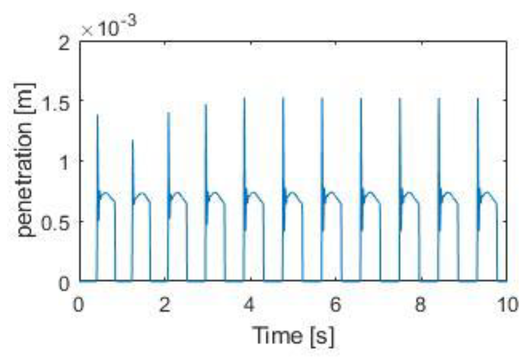
The penetration can be seen in Figure 8, and the normal force can be observed in Figure 9. It can be observed how the period of these graphs is the same as the period obtained from the experiment. In both of these figures, it can be observed that, as there is a great initial impact when the foot hits the ground, this causes a large penetration, for an instant of time, and after that initial impact the values are stabilized. This impact/impulse is transmitted from one foot to the other one, in some cases causing bounces, instability or chaos. It is also observed that when the foot is in the air, it does not suffer a normal force or cause penetration. These graphs are one foot, and the graphs of the other foot would be symmetrical.

4. Numerical Results and Discussion

In this part, we aim to discuss some interesting results, including robustness, stability and efficiency.

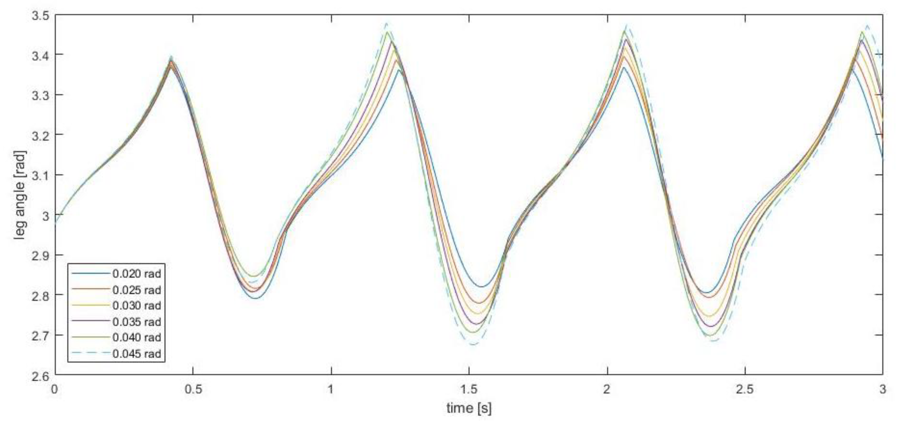
First, the effect on the slope has been investigated. The hip speed of the model along the slope varies every time during the walking. In Figure 10, the leg angle for different slopes can be appreciated. It can be noted that for the slope of 0.20 rad, the walking is steady and fully passive. At a higher slope, the leg angle increases with every step, gaining kinematic energy. That is to say that all the gravitational potential energy that is gained is greater than the energy that falls on each impact, with which its kinetic energy increases at each step. These results are as expected.

The main numerical methods to solve the equation of motion commonly used in multibody dynamics systems have been applied to the model. This section also presents a comparative analysis of various methods to control the constraint violations.

Seven problem-solving methods have been applied, namely the standard Lagrange multipliers method (standard), the baumgarte stabilization approach (baumgarte), the penalty method (penalty), the augmented lagrangian formulation (augmented), the index-1 projection method (index1), the index-1 augmented lagrangian method (index1aug) and the direct correction method (described).

For this comparison, the differential and algebraic equations of motion of the multibody dynamics system will be solved with the most popular and used numerical integration methods: First, the ode integrator scheme; second, the Euler integrator scheme, and third, the second-order classic Rung-Kutta methods are utilized. These methods have been known for more than 100 years, but their potential was not fully realized until computers became available. All the cases are simulated and analyzed for the same period, and with the same initial conditions.

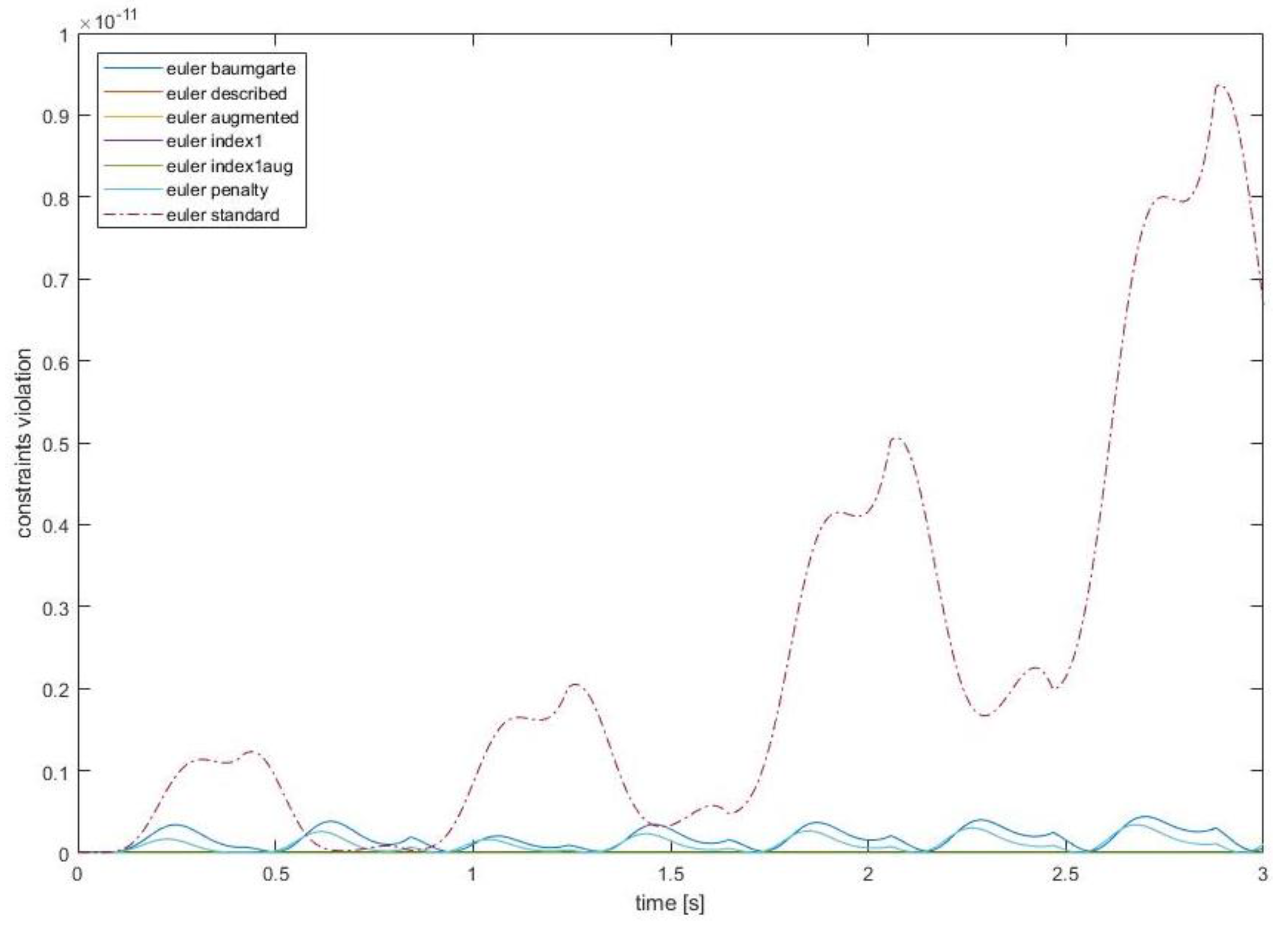
Figure 11 displays the position constraints violation for all the methods, and Figure 12 shows all the methods except the standard one. The scale in Figure 11 is different from the scale in Figure 10. In this analysis, all the methods named above (standard, baumgarte, augmented, penalty, index1, index1aug and described) are utilized to solve the dynamics system.

It can be seen that the constraints violations are getting out of control with the standard method. Nevertheless, with the other methods (baumgarte, augmented, penalty, index1, index1aug and described) the constraint violations remain under control indefinitely. It can be observed that the constraints violation of the augmented lagrangian formulation, baumgarte stabilization approach and the direct correction approach have the same order of magnitude and that the results are similar.

With these results, the robustness of the model has been demonstrated. It works properly with all the methods.

Figure 13 compares the computational time for different solving methods. The standard method (standard lagrange multiplier) is the most efficient. Moreover, the augmented lagrangian formulation and the baumgarte stabilization approach present a similar time ratio. These two methods have much fewer constraints violations when compared with the standard one. It can be concluded, for this particular model, that the best resolution methods in terms of efficiency are the standard, baumgarte and augmented ones.

In the previous paragraph, the equations of motion for the dynamics model were derived and integrated with the Euler integration method. As seen in the results, the augmented method has the constraints violation under control, and the efficiency is similar to that of the standard methods. Then, the integration methods have been compared using the augmented method and the standard. In Figure 14, the Ordinary Differential Equations, “ODE”, integrator, the “Euler” and the Runge-Kutta, “runge2”, are compared using the augmented method. It should be noted that the three graphs have very different orders of magnitude, and that the method that best eliminates the constraints violations in this passive walking model is the Runge-Kutta.

Furthermore, the same comparison has been made with the standard method, achieving similar results. This is shown in Figure 15, where it is easy to check that the Runge-Kutta integrator controls the constraint violations better. It should be noted that the three graphs have very different orders of magnitude.

The efficiency of the different integrators applied to solve the dynamics model are presented in Figure 16. As was expected, the Runge-Kutta integrator (with both methods: standard and augmented) is the less efficient approach. It needs more operations to control the constraints violations. Moreover, the ode integrator needs much less time than the Runge-Kutta or the Euler integrator. With these results, it can be concluded that, for this model, the combination of the augmented method with the ode integrator is a good approach, keeping the constraints violation under control with a low computational cost.

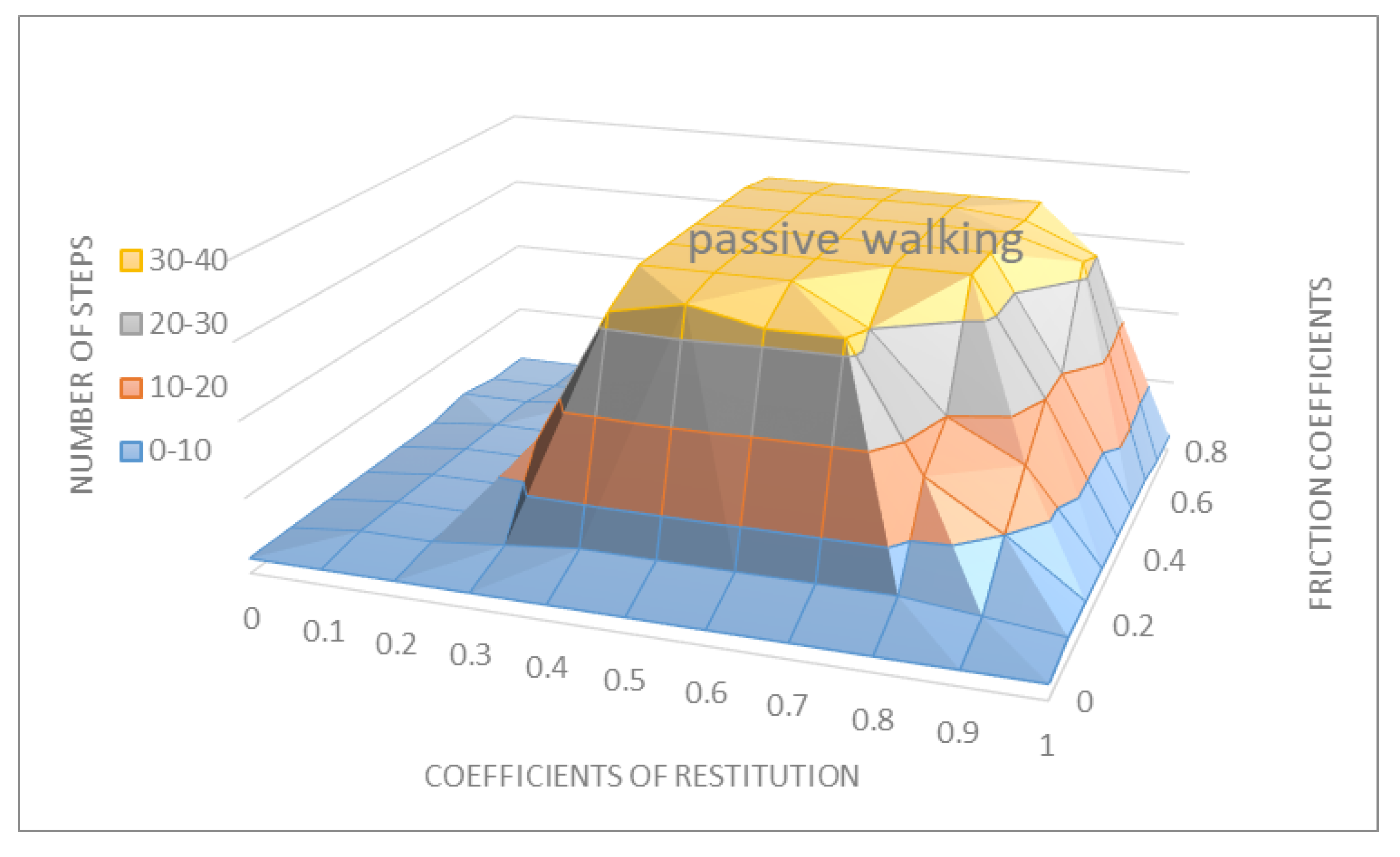
In order to obtain interesting results, a sensitive analysis has been made. In the simulations, it has been observed that with a bigger value of contact stiffness, the penetration-deformation of the ground-feet decreases. With a constant of damping sufficiently large, the walking feet do not bounce with the ground. If the constant of damping is reduced to a small enough value, there will be vibrations, and the model will fall. In order to see the relation between the stiffness and the damping, different coefficients of restitution are compared in Figure 16. In the simulations, it has been seen that the length of the walking gait and the average velocity rises with the increasing of the stiffness, but the gait continues with a passive stability. All of this can be checked with the present model.

In addition, it can be observed that the variations of the constant of damping on the passive biped has no significant effect on the walking stability. This is a very interesting result: A biped passive gait does not change after the contact damping increases to a large value, whereas with a very small value the model will not be able to walk. The average velocity decreases as the contact stillness increases. As we can see in Figure 17, an increase in the friction coefficients does not change the walking gait; otherwise, a decrease in the friction coefficients decreases the biped models’ stability. With these results it can be concluded that with this weight and this slope, and with a sufficiently high value of the damping factor, the biped will be able to move in a passive walking way.

5. Conclusions

The supporting foot slippage and the viscoelastic dissipative contact force of the passive walking biped has been studied and modeled. The smooth forward dynamics model for the whole walking is presented and verified. Several contact forces and friction forces are compared, demonstrating that the ones that work best in a passive biped model are the Flores contact/impact normal force and Bengisu friction.

Knowing that the model works properly, a sensitivity analysis has been carried out, obtaining interesting results with different numerical methods to solve the equation of motion (standard, augmented, baumgarte, penalty, the index-1 and direct) and different integrator schemes (ode integrator scheme, Euler integrator scheme and the Runge-Kutta methods). These results have shown their consistency. With these results, it can be concluded that, for this model, the augmented method or baumgarte method, combined the Runge-Kutta integrator, is a good solution, keeping the constraint violations under an intimate value with a low computational cost.

This model can be implemented in parametric programs, rendering the opportunity to carry out simulations of different mechanisms, bipeds, robots and machines possible. We believe that this is an important contribution to the scientific community. The results show the robustness and reliability of this dynamic model with impact and friction. Thus, this same method could be used to develop other models with impact and friction and obtain reliable simulations.

Some of the most interesting results that have been obtained with the simulations of the model are: In this research, it is easy to see that there is a proportional relationship between mechanical work (gravitational potential energy) and metabolic/passive cost (impacts). We can conclude that a lower contact stiffness and sufficiently high coefficient of restitution correspond to soft feet and the biped walking more steadily. The damping factor does not change the stability of the passive biped walking; it influences the bounce between the feet and the ground. With a very low and very high constant of damping, the biped bounces too much and becomes unstable. The friction coefficient is only related to the slippage. For a very small coefficient of friction, the walking biped slips. The changes of the stiffness value modify the dissipation energy and the time-period (the walking length is larger).