1. Introduction
One important problem in the operation of many industrial manipulators is the transmission of vibrations to the fixed frame during their high-speed motion. These vibrations are produced by the unbalanced inertia forces that increase the shaking force and shaking moment. Thus, a traditional and still very important research topic in robot design is finding new methods to remove or decrease these alternating dynamic loads transmitted to the base And, in this way, to reduce wear, allowing to increase the operating velocities.
The shaking force balancing, i.e., the reduction or, in the best case, elimination of the variation in the force transmitted to the base, is a problem that has been solved in different ways. One of the most popular and effective is mass redistribution. This method proposed by different authors was successfully introduced in Reference [
1] using the “linear independent vectors” method. In general terms, the objective is to find the appropriate location of the center of mass of the links of the mechanisms in order to make the general Center of Mass (CoM) stationary for any motion of the manipulator.
Practical ways to move the CoM of the system and to make it stationary have been to add a set of counterweights [
2,
3,
4,
5], to add auxiliary structures [
6,
7,
8,
9], or to modify the form of the links from the early design phase [
10,
11,
12]. A comprehensive review of the methods with illustrative examples can be seen in Reference [
13]. Specific applications to robotics can be seen in Reference [
14,
15,
16,
17,
18,
19,
20], and a review of these kinds of applications is in Reference [
21].
However, all these methods imply a considerable increment in the mass of the system, causing the shaking moment and, hence, the driving torque to grow; see Reference [
22]. An additional drawback of these methods is that they also imply modification of the original system, making its application somehow hard or complicated, leading to relatively complex mechanical systems increasing their size.
Recently, a new approach has been proposed. It is based on the optimal control of the manipulator global CoM [
23,
24]. The method is based on planning the displacements of the total CoM of the moving links. Its trajectory is defined as a straight line with “bang-bang” motion profile, ensuring solely the initial and final positions of the end-effector. This approach allows the reduction of the maximum value of the acceleration of the CoM, leading to a reduction in the shaking force.
In this work, this approach is resumed and presented using fully Cartesian coordinates, also known as natural coordinates [
25]. The application of natural coordinates to the dynamic balancing of mechanisms in the plane has been explained in Reference [
26]. An application to obtain the balancing conditions of planar mechanisms is described in Reference [
27]. A specific application to the dynamic balancing of the four-bar mechanism, explaining the way to obtain the dynamic reactions to be used in an optimization procedure, can be found in Reference [
28]. Initial efforts to use this approach to obtain the balancing conditions in spatial mechanisms can be seen in Reference [
29].
The methods presented in References [
23,
24] use reference-point coordinates to calculate the position of the global CoM. Then, this position has to be expressed in terms of the degrees of freedom and some convenient relative coordinates. In this process, the kinematic constraints (vector closed-loop equations) that relate the reference-point coordinates and the selected relative coordinates are used. The process becomes somehow cumbersome when dealing with closed-loop mechanisms, especially in three-dimensional space.
One advantage of using fully Cartesian coordinates is that, in complex multibody systems, points and vectors can be chosen at the joints usually shared by contiguous bodies, contributing to a definition of joints with few or no constraint equations while keeping moderate the number of variables. Thus, the expressions necessary to calculate the general CoM, the shaking force, and the shaking moment of the system can be obtained in a direct and automated way. Another advantage is that the force balancing conditions, directly expressed in terms of the local coordinates of the CoM of the bodies, are obtained directly from the terms in the mass matrix. In the authors’ perspective, this contributes to making the method based on the optimal control of the robot-manipulator center of mass faster and easy to perform.
In this article, the natural coordinates are used to obtain the analytical expressions to calculate the position of the general CoM, the shaking force, and the shaking moment of the 3RRR planar parallel manipulators (PPM).
The expressions to calculate the shaking force are used for the force balancing of the mechanisms applying the method based on the optimal control of the global CoM of the manipulator, as presented previously in References [
23,
30,
31]. As a first approach, the acceleration of the global CoM is reduced using “bang-bang” law, proposing to partially balance the the manipulator without any addition of supplementary masses. As a second approach, a two-stage method is proposed. The first stage consists of the optimal redistribution of the driving links’ masses using counterweights, securing convergence of the end-effector trajectory and the CoM of the manipulator. This mass redistribution is done without increasing the total mass of the original system, keeping the masses of the driving links the same value. In a second stage, the optimal control of the end-effector acceleration according to the “bang-bang” law is developed. The expressions for the shaking moment are used to verify the behavior of the mechanism before and after the force balancing.
The rest of the article is organized as follows: in Section two, a description of the modeling using fully Cartesian coordinates (natural coordinates), stressing the importance of the mass matrix of the body, is presented. Special attention is given to the mass of a link represented with two and three “basic points”. Additionally, a general and easy to automate method to calculate the global CoM, the shaking force, and the shaking moment is introduced. In Section three, the method described in Section two is applied to calculate the shaking force balancing conditions of the 3RRR PPM and the partial force balancing following the approaches described in the previous paragraph. In Section four, all analytical expressions developed in Section three are used in a numerical example for an specific manipulator. Comparative results from computer simulations are presented. Finally, conclusions are given in Section five.
2. Modeling Using Fully Cartesian Coordinates
The idea behind the fully Cartesian coordinates, also known as natural coordinates, is to use the Cartesian coordinates of a set of appropriate points, the “basic points”, to define the position of a solid in the plane or in the three-dimensional space. These coordinates are dependent, related by the rigid body conditions that keep constant distances and angles. The kinematic constraint equations can be formulated using the scalar product (dot product) of vectors, leading to quadratic constraint equations and linear terms in the Jacobian matrix.
The core application of this kind of coordinates is that, in a complex system, points can be shared between contiguous bodies. This contributes to the definition of joints with few or no additional constraint equations. Thus, a single set of variables define the position and the geometry of the bodies, directly in the global reference frame [
32].
From the dynamics point of view, the mass of the bodies can be distributed among the points used for the model. These punctual masses are then related by the general mass matrix that holds implicitly the kinematic relations when properly assembled. This allows to treat the system as a cloud of moving points, avoiding the use of angular coordinates and consequently the direct use of the moment of inertia. Thus, the key point of the modeling technique is the assembly of the mass matrix of the system.
2.1. Mass Matrix of a Body in the Plane
When dealing with mechanical systems in the plain, natural coordinates introduce a set of points to define a body, two “basic points”; see [
25] for a detailed explanation. These points concentrate the mass of all the bodies in the mechanical system in accordance to their relation among each other, expressed though the mass matrix. To calculate or assemble the mass matrix of the system, it is necessary to calculate the mass matrix of the elements first.
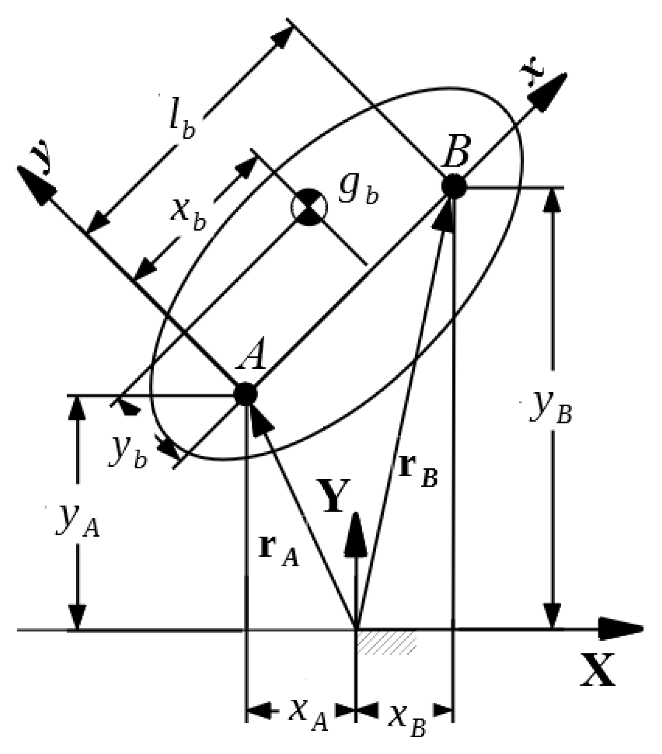
In planar systems, the standard model of a body is made with a pair of points, for example,
A and
B, as seen in
Figure 1. In this figure, it can be noted an inertial fixed reference frame
and a local reference frame
attached to the moving body at the basic point
A, its origin. It is also noted that the second basic point
B has its position in local coordinates at
and that the CoM of the body, point
, has local coordinates
.
Considering that the body
b has its mass concentrated at
equal to
and that its polar moment of inertia with respect to the origin of the local reference frame (point
A) is
, it is possible to distribute the whole mass into the basic points
A and
B to form the constant mass matrix of a body as follows:
where:
Note that
can be expressed in terms of the mass
; thus, the mass matrix can be expressed solely in terms of the mass of the body. This matrix has been obtained by applying the virtual power method, leading to a direct formulation of the inertia forces [
25].
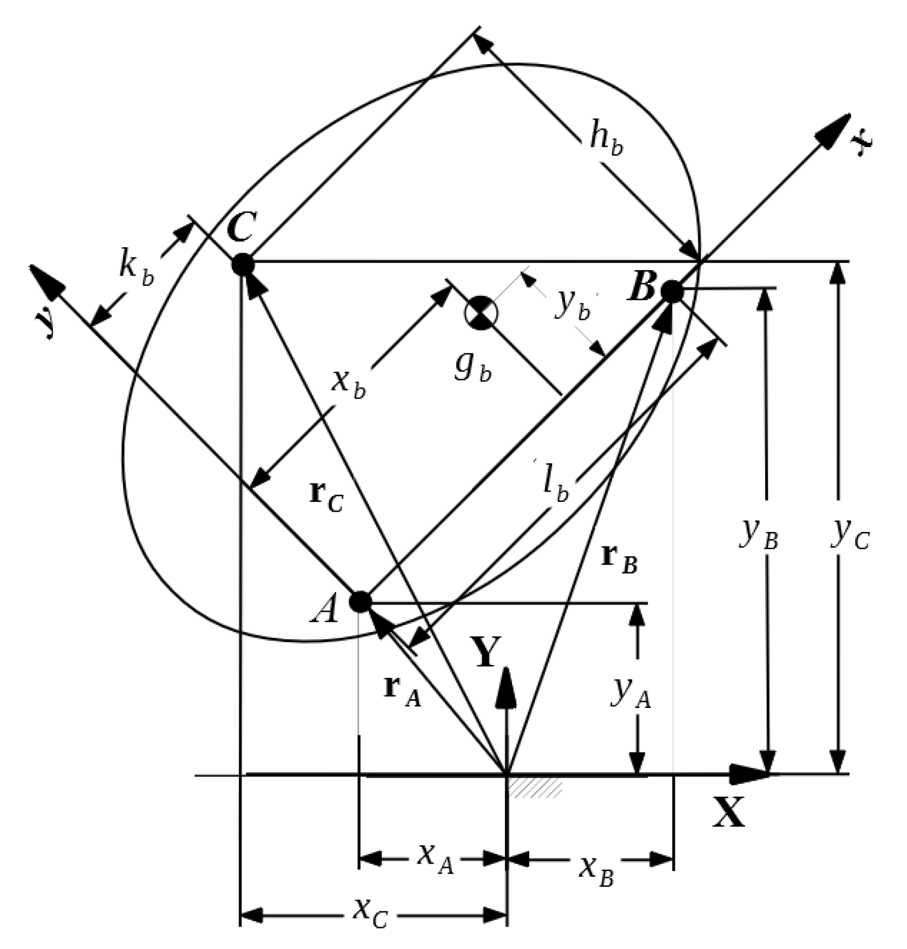
Special Case of a Body with Three “Basic Points”
A model of a body with a greater number of points could be also useful. In this case, to complete the model of the 3RRR PPM, it was required to develop the mass matrix of a body with three “basic points”; see
Figure 2.
Considering that the body
b in
Figure 2 has its mass concentrated at
equal to
and that its polar moment of inertia with respect to the origin of the local reference frame (point
A) is
, its moment of inertia with respect to the
x axis is
and its moment of inertia with respect to the
y axis is
. It is possible to distribute the whole mass into the basic points
, and
C to form the constant mass matrix of a body as follows:
where:
Note that
can be expressed in terms of the mass
; thus, the mass matrix can be expressed solely in terms of the mass of the body. In the same way as for the mass matrix in the model with two “basic points”, this mass matrix has been obtained by applying the virtual power method [
25].
2.2. Calculation of the Global Center of Mass of the System
When the model of a body is made with a pair of “basic points”, a vector of four coordinates
representing the positions vector of body
b is introduced and can be expressed as follows:
where
and
are the position vectors of points
A and
B, respectively.
In this way, the position
of the CoM of body
b with respect to the global reference frame can be calculated by the following:
In matrix form, it can be expressed as follows:
where the matrix
is introduced here to arrange the terms of the matrix multiplication to obtain the result in Equation (
16). This matrix is composed by a set of
identity matrices,
, that in number are equal to the number of basic points involved in the multiplication. In this case, matrix
is as follows:
As aforementioned, the system can be seen as a cloud of points coming from the corresponding model of each body. Thus, for a system with
n bodies, the general position of the CoM,
, can be calculated by the following:
where the total mass of the system,
m, is:
Using the points shared among bodies and following a proper assemblage procedure, the global CoM of the system can be calculated in a simple and easy to automated matrix multiplication as follows:
The terms in Equation (
21) will be exemplified in following sections by examples. The assembling procedure will be clear then.
2.3. Calculation of the Shaking Force of the System
Once the location of the global CoM of the system in Equation (
21) is defined, its linear momentum can be calculated as its time derivative in a straightforward way:
noting that
and
are constant matrices. The vector
represents the time derivatives of the coordinates in
, meaning the velocities vector. The vector
represents the velocity of the CoM of the system.
The shaking force of the system is in turn the time derivative of the linear momentum. Thus, in this case, the shaking force,
, can be calculated in a direct form as follows:
where
is the vector of accelerations of the coordinates of the points in the system, the accelerations vector, and where
is the acceleration of its CoM. It is important to note that some points are fixed; thus, its acceleration is zero. This simplifies the calculation in Equation (
23).
2.4. Calculation of the Shaking Moment of the System
The shaking moment can be calculated as the time derivative of the angular momentum of the system. The angular momentum can be calculated straightforward, noting that the system is composed solely of a cloud of points. Thus, the angular momentum,
, can be calculated by the following:
where
p is the total number of points in the system,
is the position vector of point
i,
is the velocity vector of point
j, and
is the corresponding element of the mass matrix of the system at row
i and column
j. Note that the mass matrix is symmetric.
The angular momentum in Equation (
24) can be expressed in matrix form as follows:
where
is a row vector representing all the vector products in Equation (
24) and has the following form:
where
.
The shaking moment,
, can be obtained by the time derivative of Equation (
25) and can be expressed as follows:
where
and
. It is important to note that some points are fixed; thus, their velocities and accelerations are zero, simplifying the calculation in Equation (
27). This advantage will be illustrated in the following sections with the application to a PPM.
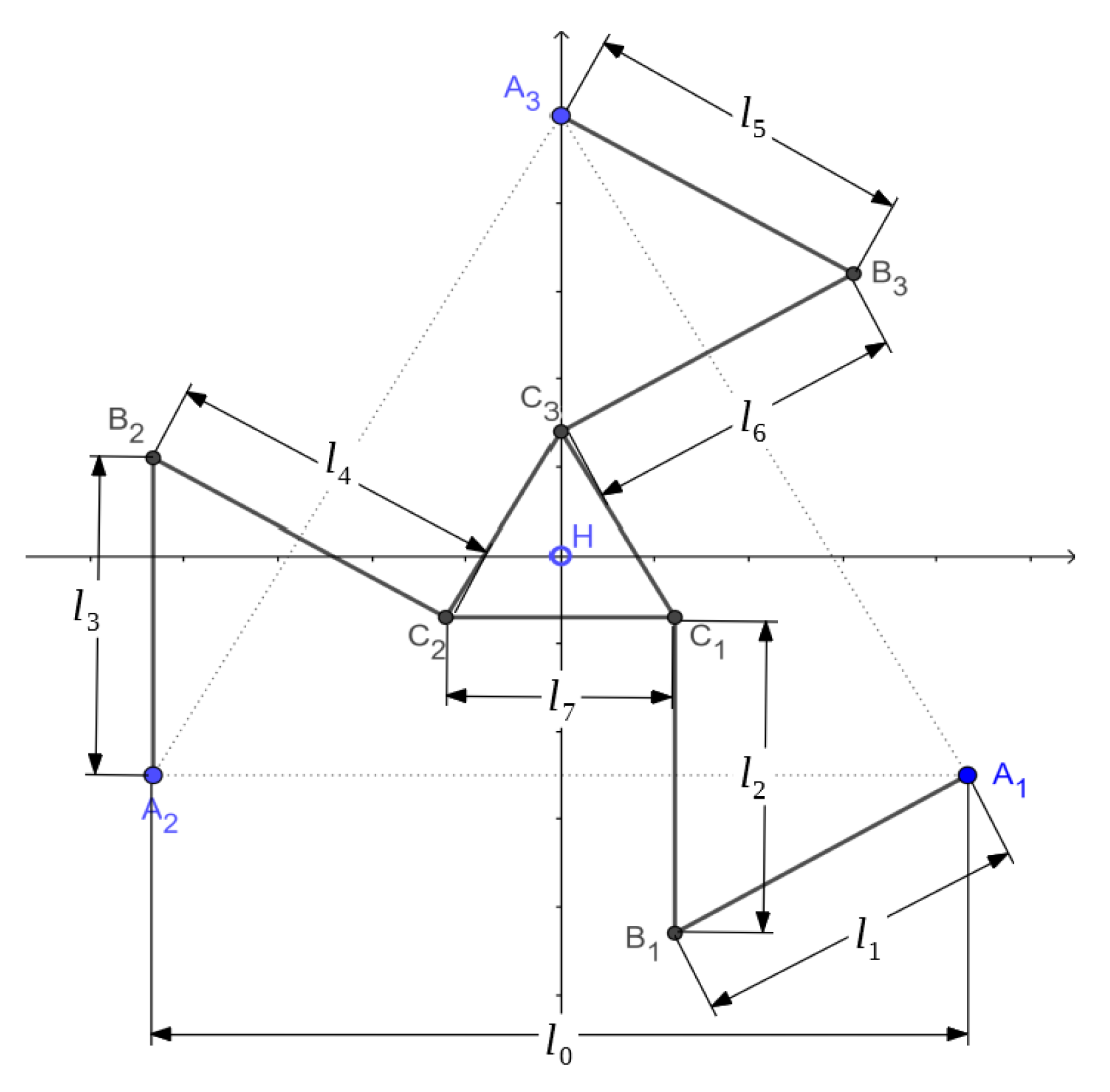
3. Generic Model of the 3RRR PPM
In this case, the model of a 3RRR PPM manipulator, represented in
Figure 3, is presented using fully Cartesian coordinates (natural coordinates), taking full advantage of this technique to obtain the global CoM position, the shaking force, and the shaking moment, as explained in
Section 2. These equations in conjunction with the kinematic equations—positions, velocities, and accelerations—are used to develop a new and general procedure to solve this kind of problem either for planar or spatial mechanisms.
3.1. Kinematic Model of the 3RRR PPM in Fully Cartesian Coordinates
The fixed platform is an equilateral triangle defined by three points: , and . The mobile platform is also an equilateral triangle defined by points: , and . The three limbs, with two links each, are defined by points ; ; and , respectively. As it can be seen, all “basic points” in the model—, and —are shared among the bodies. Point H represents the end-effector and is not part of the “basic points”.
These points introduce a vector,
, of 18 Cartesian coordinates:
where
,
. Note the way that the coordinates are organized. This is very important in the assemblage procedure of the mass matrix of the system. Any order is possible, but once selected, it must be maintained throughout all the calculation. Vector
constitutes a set of dependent Cartesian coordinates related by a set of constraint equations.
3.1.1. Constraint Equations and Solution to the Positions Problem
The manipulator has three degrees of freedom; thus, the dependent coordinates in
are related by a set of 15 constraint equations, obtained from the constant distant condition among bodies. The vector of constraint equations,
, is presented in Equation (
30).
Note that the equations in Equation (
30) are nonlinear but quadratic, very simple, and easy to differentiate to get the a linear Jacobian matrix. Thus, the solution of the positions problem though numerical iterative procedures could be faster with the aid of symbolic computing software.
3.1.2. Solution to the Velocities Problem
The velocities problem can be solved differentiating Equations (
30) with respect to time as follows:
where
is the Jacobian matrix and where
is the vector of velocities of the Cartesian coordinates:
where
, and
. The equations in Equation (
31) are linear simultaneous and lead to the solution of the velocities problem.
3.1.3. Solution to the Accelerations Problem
The accelerations problem can be solved differentiating Equation (
31) with respect to time as follows:
where
is time derivative of the Jacobian matrix and where
is the vector of accelerations of the Cartesian coordinates:
where
and
. The equations in Equation (
33) are linear simultaneous and lead to the solution of the accelerations problem once positions and velocities are known.
3.2. Calculation of the Global CoM Location
To calculate the global CoM location, Equation (
21) can be used. It is necessary to calculate or assembe the global mass matrix first. Thus, it is important to note that point
is shared by bodies 1 and 2, point
is shared by bodies 3 and 4, point
is shared by bodies 5 and 6, point
is shared by bodies 2 and 7, point
is shared by bodies 4 and 7, and point
is shared by bodies 6 and 7. In this case, following the same order specified in the positions vector, Equation (
29), the
mass matrix is assembled as follows:
In this case, matrix
has nine
identity matrices:
Multiplying the terms in Equation (
21) and simplifying, the final expression to calculate the global CoM position is as follows:
where
As it can be seen, the matrices in Equations (
38)–(
46) are constant and depend solely on the masses of the bodies. Thus, the global CoM changes with the change in position of the Cartesian coordinates in the model.
3.3. Calculation of the Shaking Force
Deriving Equation (
37) once with respect to time, it is possible to calculate the linear momentum of the manipulator. Noting that
, the linear momentum is expressed as follows:
where
is the linear momentum and
is the velocity vector of the global CoM. This equation, along with Equation (
31), is very useful to solve the velocities problem.
To calculate the shaking force of the system, it is necessary to simply derive Equation (
37) twice with respect to time. In this process, we have to note that
; thus, the shaking force can be expressed by the following:
where
is the shaking force and
is the acceleration vector of the global CoM.
3.4. Calculation of the Shaking Moment
To calculate the shaking moment of the manipulator, it is possible to use Equation (
27). It is important to take into account that the velocities and accelerations of points
, and
are zero. Multiplying and simplifying the terms in Equation (
27), it is possible to write the following:
where, in this case,
and
4. Shaking Force Reduction of the 3RRR PPM
In this section, the partial shaking force balancing of the 3RRR PPM is presented. The solution is proposed with two different approaches:
The first one is based on the optimal trajectory planning of the common CoM of the manipulator, which is carried out by “bang-bang” profile. This approach was introduced in Reference [
13] and applied to a 3RRR PPM in Reference [
31].
The second one is implemented in two stages: the first stage consists of the optimal redistribution of the driving links’ masses using counterweights, reaching the convergence of the end-effector’s trajectory and the global CoM of the manipulator. The second stage consists of the development of an optimal control of the end-effector’s acceleration according to the “bang-bang” law. A solution using this approach has been presented in Reference [
30].
Unlike the solutions presented in References [
30,
31], in this case, the equations derived in the previous section were used, pointing out the calculation procedure as well as the advantages.
The application of the method developed in the previous section is illustrated with an specific 3RRR PPM, with the mass and length parameters specified in
Table 1. The fixed points of the manipulator are located according to the following values:
,
, and
; see
Figure 3.
4.1. Optimal Trajectory Planning of the Common CoM
A common problem in robotics is to impose a trajectory to the end-effector in order to comply with a specific task. In a simple way, without regarding the obstacle avoidance and the singular positions, this is done by defining the initial point and the final point of the tool’s trajectory and then by applying a feasible law of motion between them. Usually a straight line imposes the appropriate velocity and acceleration conditions at the beginning and at the end.
If a cycloidal motion is imposed, assuring zero velocity and zero acceleration at the beginning and at the end of the trajectory, the motion law completed in a total time T and traveling a total distance L can be expressed as follows:
where
S is the distance traveled in function of time.
In this case, a manipulator with the parameters defined in
Table 1 is moved from the initial position of the end-effector,
, to the final position,
, in a total travel time
. The straight line trajectory of the end-effector is represented in
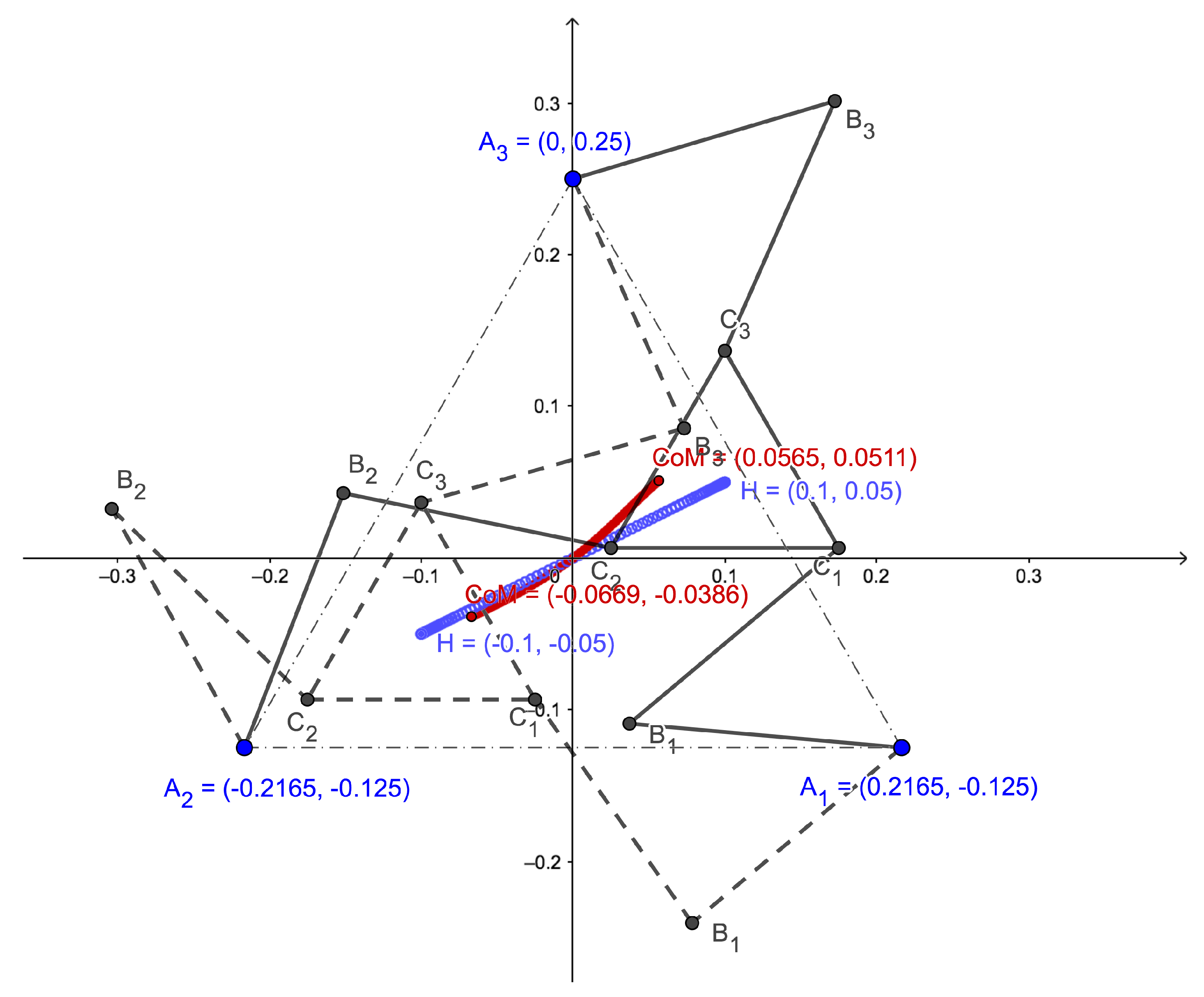
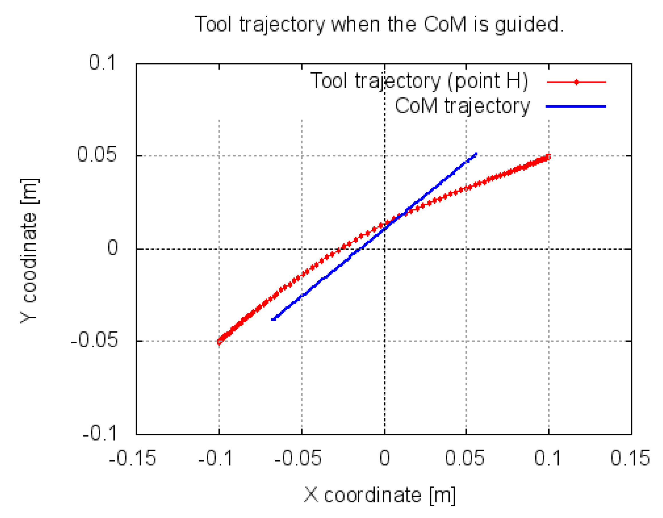
Figure 4. The trajectory followed by the CoM is also presented. Note that there is a nonlinear relation between the motion of the manipulator’s tool and its CoM.
Note also that, for the initial position of the end-effector, point , the corresponding position of the manipulator’s global CoM is , while for the final position of the end-effector, point , the corresponding position of the manipulator’s global CoM is .
To calculate the global location of the CoM corresponding to a specific point of the tool, it is necessary to solve the initial position problem. This consists of determining the position of all the “basic points” in the system by knowing the positions of the fixed and input points, which can also be called guided or driven points, in this case, point
H. Mathematically, the initial position problem in this case is reduced to calculate the position of the CoM corresponding to the input coordinates of the end-effector by solving the set of nonlinear Equations (
30) and (
37) simultaneously.
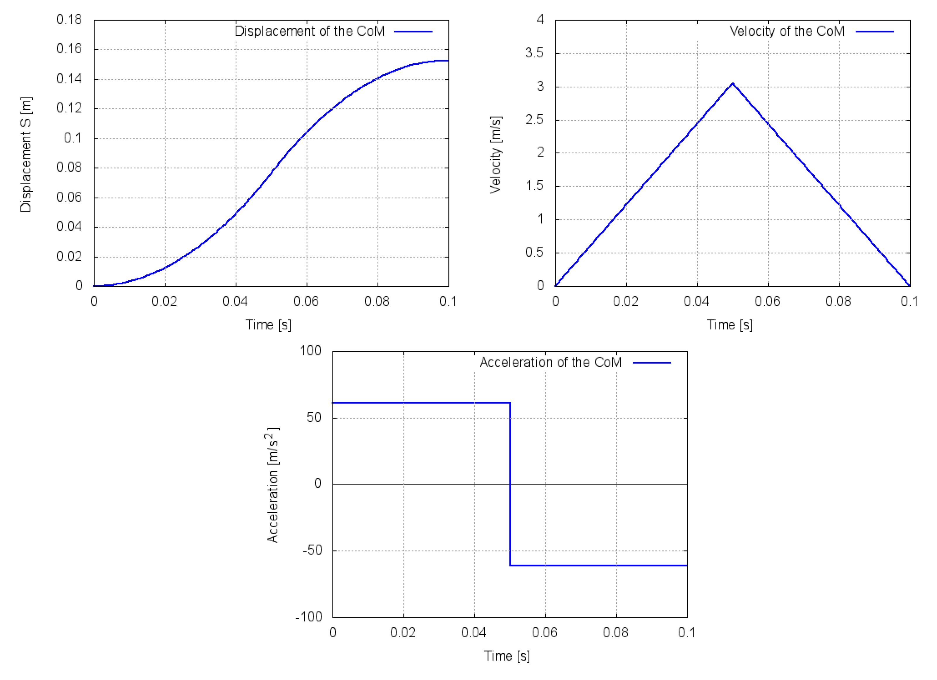
Conversely, now, it is desired to guide or drive the CoM of the manipulator to generate a corresponding trajectory for the end-effector. In this case, the trajectory imposed to the global CoM from its initial position to its final position follows a “bang-bang” profile as presented in
Figure 5.
To calculate the trajectory of point
H, corresponding to the defined trajectory of the CoM, it is necessary to solve the set of nonlinear equations in Equations (
30) and (
37) simultaneously for the known positions of the CoM. In this case, the resulting trajectory is presented in
Figure 6.
As it can be seen in
Figure 6, the trajectory of the CoM is a straight line. The corresponding trajectory of the end-effector of the manipulator is not straight; there is no linear relation between both trajectories. Note that, doing this, it can only be assured the initial and the final position of the original trajectory of the tool.
Once the positions of the manipulator are solved using Equations (
30) and (
37), it is possible to solve velocities and linear momentum, using Equations (
31) and (
47) simultaneously. Note that this new set of equations is linear; no iterative solution is required. Once the positions and velocities are known, it is possible to calculate the accelerations and the shaking force solving simultaneously Equations (
33) and (
48). Note again that this set of equations is linear.
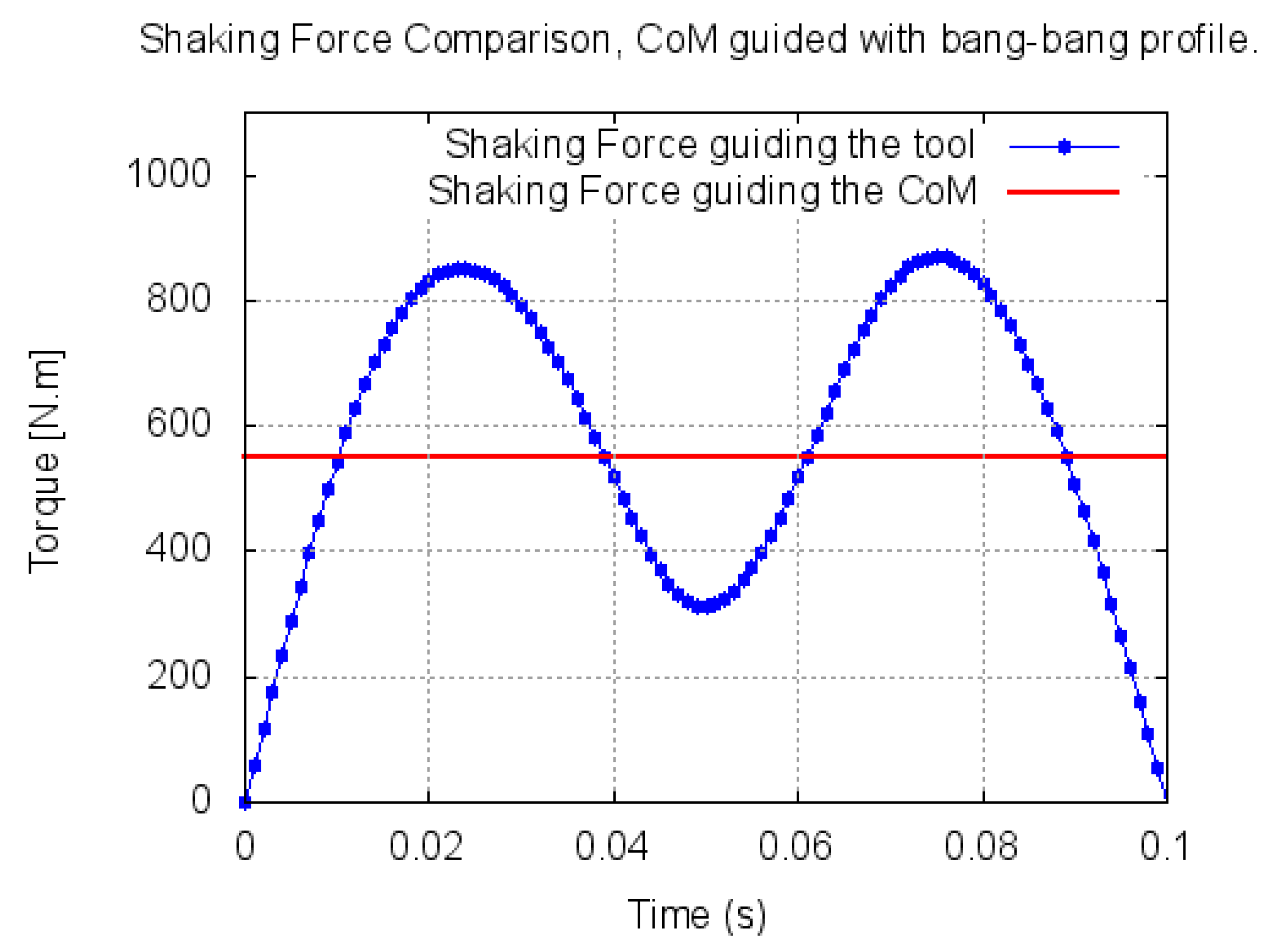
The result from guiding the CoM with a “bang-bang” profile, assuring a constant acceleration during its motion, is an elimination of the variation of the shaking force and a reduction in its magnitude as it can be seen in
Figure 7.
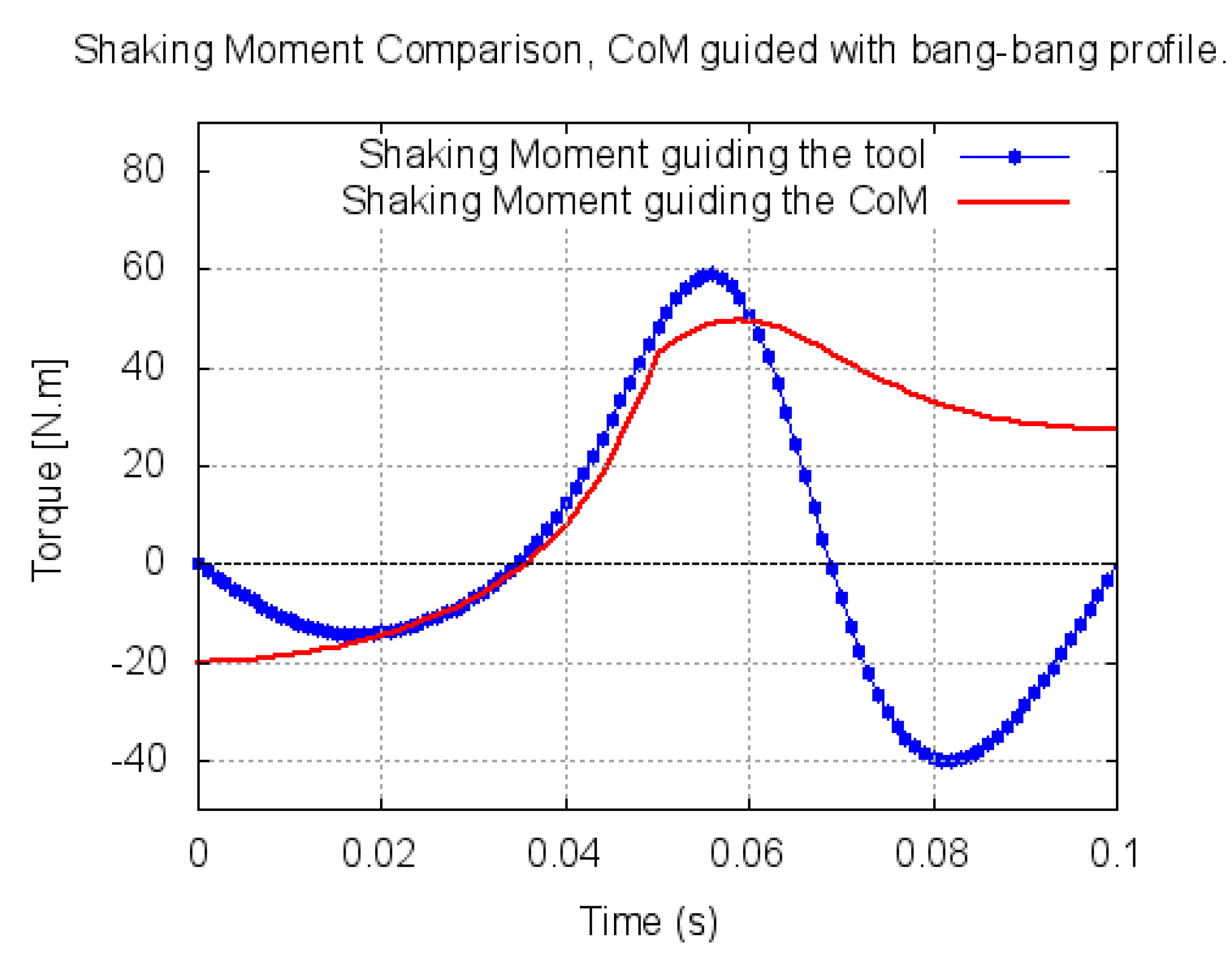
Once the positions, velocities, and accelerations of the “basic points” are solved, it is possible to calculate the shaking moment using Equation (
49). Although guiding the CoM, assuring a constant acceleration, is focused on the elimination of the variation of the shaking force, it can also contribute to the reduction of the shaking moment and its variation. A shaking moment comparison is presented in
Figure 8. The moment is calculated with respect to the origin of the global reference frame shown in
Figure 3.
4.2. Redistribution of the Driving Links’ Masses
A second strategy is to eliminate the variation of the shaking force of the manipulator following a two-stage procedure. The first stage is to redistribute the mass of the driving links in order to get a linear relation between the motion of the end-effector and the motion of the global CoM.
This can be done by eliminating all the terms (making them equal to zero) in the matrices—
and
—described in Equations (
39), (
42) and (
45); thus, Equation (
48) can be changed to calculate the shaking force as follows:
Note that, in Equation (
53), the terms in matrices
, and
are constant. Additionally the motion of points
, and
can be expressed in terms of the motion of point
H and the rotation of the mobile platform (body 7). In this way, a linear relation between the motion of the end-effector and the motion of the CoM is achieved. Thus, assigning a “bang-bang” profile to the trajectory of the the tool and solving the corresponding inverse kinematics problem, it is possible to determine the motion of the driving motors, a very common problem in robotics.
As an advantage of using fully Cartesian coordinates modeling, it can be pointed out that the necessary conditions to redistribute the mass among the driving links are expressed directly in terms of the mass and the location of the CoM of the links 1 through 6. The conditions related to limb 1 are as follows:
The conditions related to limb 2 are as follows:
Finally, the conditions related to limb 3 are as follows:
The easiest way to comply with the conditions of Equations (
55), (
57) and (
59) is having the CoM of links 2, 4, and 6 inline between their respective joints. This is the case of the manipulator illustrated in this example; see the parameters in
Table 1.
To comply with the conditions in Equations (
54), (
56) and (
58), it is proposed to leave links 2, 4, and 6 as they are and to relocate the CoM of the driving links 1, 3, and 5 by adding counterweights or by changing their form (redistribution of mass). In this case, all links are equal; thus relocation of the CoM of the driving links can be done alike for the driving links. In this case, the relocation of the CoM in these links is achieved just by moving them in the
x direction, keeping the following relation:
where
and
.
To keep the explanation of the method simple and to not distract attention from its application, the mass of the driving links are maintained in the same value:
. Thus, the new location of the CoM of the driving links can be calculated by substituting values in Equation (
60) as follows:
With these new parameters, a “bang-bang” motion profile to the straight line trajectory of the end-effector is imposed from its initial point
to its final point
.
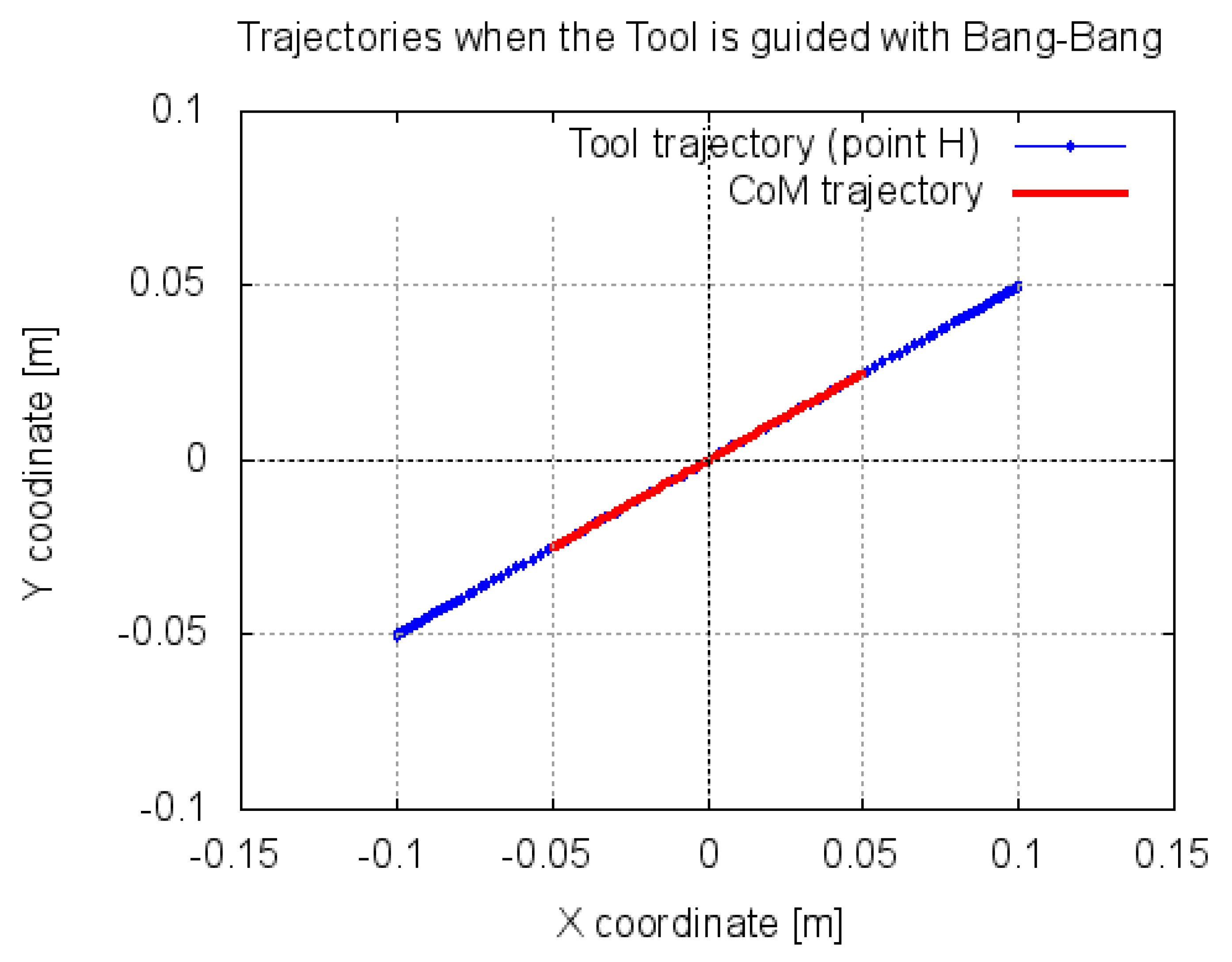
Figure 9 shows the trajectories generated for the tool and for the CoM. Note the linear relation between them; the trajectory of the CoM is exactly over the trajectory imposed to the end-effector.
Once the positions of the manipulator are solved using Equations (
30) and (
37) as in the previous case, it is possible to solve velocities and linear momentum. Then, it is possible to calculate the accelerations and the shaking force solving simultaneously Equations (
33) and (
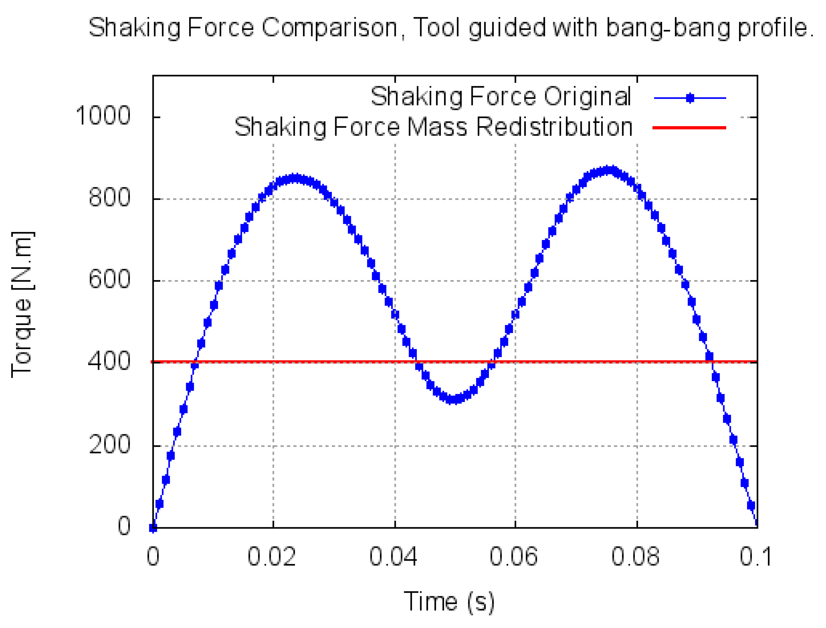
53). Note that this set of equations is linear. The corresponding calculated shaking force is presented and compared to the original case in
Figure 10.
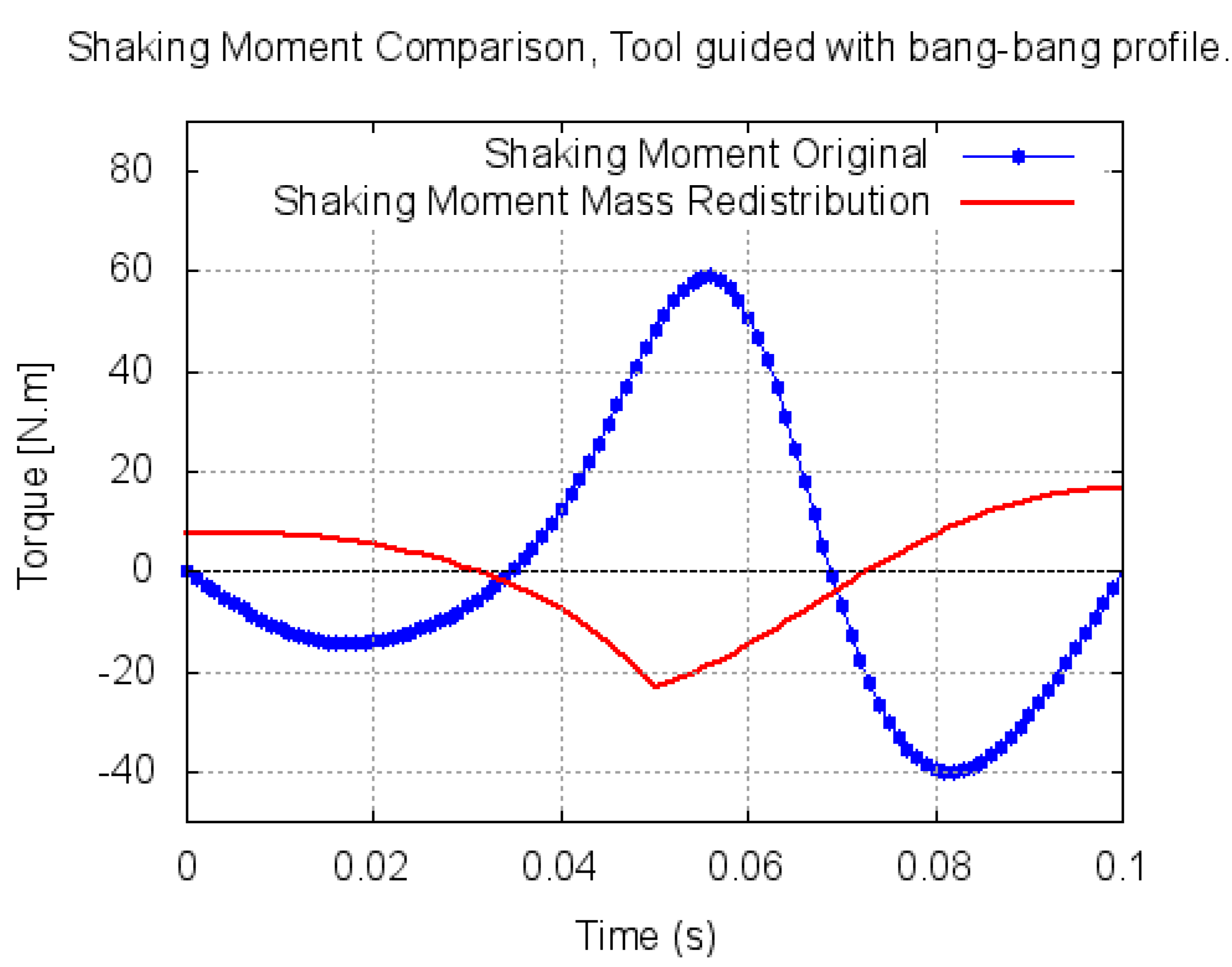
Once the positions, velocities, and accelerations are solved, it is possible to calculate the shaking moment using Equation (
49). The shaking moment comparison is presented in
Figure 11. The moment is calculated with respect to the origin of the global reference frame shown in
Figure 3.
5. Discussion
This paper has presented an alternative method, based on fully Cartesian coordinates for the modeling and generation of the shaking force and shaking moment reactions of mechanical systems in general. No angular variables were used at all. Different advantages with respect to previous modeling techniques have been pointed out, such as the ease to be automated and the direct way to get the dynamic reactions in analytical form. It has been also clear that the balancing conditions can be identified directly from the generated mathematical expressions. All these expressions are written in terms solely of the mass and of the local coordinates of the CoM of each body, making the them more clear.
The application to a 3RRR PPM is illustrated, and some interesting results have been presented. It is worth to mention that the nonlinear relation between the trajectory of the end-effector and the trajectory of the CoM of the manipulator is clearly shown. The advantages of guiding the CoM to minimize the shaking force are presented in a clear way, and the effects on the shaking moment are pointed out. Finally, the alternative of a mixed technique, combining balancing by redistributing the mass and the kinematic guidance of the end-effector using a proper motion profile, bang-bang in this case, is presented and its advantages are also shown.
This research will continue for applications in spatial parallel manipulators and mechanical systems in general. Special attention will be paid additionally to the reduction or elimination of the shaking moment, following an alternative techniques different from the redistribution of mass. Kinematic redundancy combined with actuation redundancy could be a promising direction.


