Article

A Novel Hybrid Harmony Search Approach for the Analysis of Plane Stress Systems via Total Potential Optimization

1
Department of Civil Engineering, Istanbul University–Cerrahpaşa, Istanbul 34310, Turkey
2
Department of Civil Engineering, Istanbul Beykent University, Istanbul 34396, Turkey
3
College of IT Convergence, Gachon University, Seongnam 13120, Korea
*
Authors to whom correspondence should be addressed.
Appl. Sci. 2020, 10(7), 2301; https://doi.org/10.3390/app10072301
Submission received: 27 February 2020 / Revised: 18 March 2020 / Accepted: 19 March 2020 / Published: 27 March 2020

Abstract

:
By finding the minimum total potential energy of a structural system with a defined degree of freedoms assigned as design variables, it is possible to find the equilibrium condition of the deformed system. This method, called total potential optimization using metaheuristic algorithms (TPO/MA), has been verified on truss and truss-like structures, such as cable systems and tensegric structures. Harmony Search (HS) algorithm methods perfectly found the analysis results of the previous structure types. In this study, TPO/MA is presented for analysis of plates for plane stress members to solve general types of problems. Due to the complex nature of the system, a novel hybrid Harmony Search (HHS) approach was proposed. HHS is the hybridization of local search phases of HS and the global search phase of the Flower Pollination Algorithm (FPA). The results found via HHS were verified with the finite element method (FEM). When compared with classical HS, HHS provides smaller total potential energy values, and needs less iterations than other new generation metaheuristic algorithms.

1. Introduction

In the analysis of structural members, the general trend for linear systems is to find deflections after forming a matrix equation involving the stiffness matrix, loads, and deflections. By using very elaborate matrix methods, linear equations thus formed are solved with great success. This is not the case for nonlinear systems, where the use of additional iterative methods becomes a must [1,2,3,4] since the stiffness matrix halts to be a constant one. Effectively, in those cases, the stiffness function is in turn a function of displacements. Detailed information about the optimization and design of various structure types can be found in Nazir et al. [5].
In recent years, total potential optimization using metaheuristic algorithms (TPO/MA) has been proposed as an iterative analysis method [6]. As is already known, all mechanical systems are in stable equilibrium in the case of minimum total potential energy. Thus, the minimization of the total potential energy of a system can be performed by considering the deflections as design variables. TPO/MA have been used successfully for the analysis of several structural systems. The first application area of TPO/MA is the truss structures. Different metaheuristic algorithms, such as local search [6], harmony search (HS) [7], and particle swarm optimization (PSO) [8], are employed with TPO/MA to analyze truss structures.
In TPO/MA, since the displacements are the basic unknowns of the problem, the method becomes effective in finding second-order effects directly without the requirement of an additional process. Additionally, the finding of non-unique solutions [9] and material non-linearity [10] can be easily tackled.
Different to truss structures, other truss-like systems, such as tensegric structures [11] and cable systems [12], are also solved via TPO/MA. In order to enhance the capacity of the method in solving large scale systems, hybrid metaheuristic algorithms combining the flower pollination algorithm (FPA), the teaching learning-based optimization (TLBO), and the Jaya algorithm (JA) are also proposed [13].
In this study, an innovation has been performed for enlarging the application area of the method TPO/MA to plates and plate-like structures. For this purpose, a simple approach has been adopted, which consists of dividing the system into triangles, of which the nodal displacements are the unknowns of the problem. Then, the strain energy of each triangle is expressed in terms of these variables. The summation of all these energies yields the total strain energy of the system. Adding to this value algebraically, the work done by the external forces again expressed in terms of the nodal deflections yield the total potential energy of the whole system considered. The rest of the technique is the determination of nodal displacements that will minimize the total potential energy through a metaheuristic optimization algorithm. Only plane stress problems are considered in this first trial.
According to previous studies, HS is a suitable and effective algorithm for TPO/MA. For the numerical examples of the study, HS is effective to find close values to the finite element method (FEM) results and other new generated algorithms. Additionally, HS is also a well-proved algorithm for structural optimization problems [14,15]. Several recent applications in the last decade are mentioned as follows.
Kaveh and Talatahari developed a hybrid algorithm that is based on PSO with passive congregation, ant colony optimization, and HS to solve the optimum design of plane and space truss structures [16]. An adaptive HS algorithm was proposed by Hasançebi et al., and the proposed method for the optimum design of large-scale steel frame structures has the ability to automatically adjust the algorithm parameters [17]. Martini proposed HS for structural frameworks for size, shape and topology optimization in order to conduct a multimodal optimization proposing a range of good alternative solutions instead of a single optimum one [18]. Degertekin proposed two different modifications of HS for the optimization of truss structures [19]. The sequential HS algorithm was proposed to find the shape optimization of structural systems, including frequency constraints [20]. For the control of the structures, HS-based methodologies are also perfectly applied for the placement of dampers [21], tuned mass dampers [22,23], and base isolators [24]. In structural health monitoring, Jin et al. proposed and improved HS for optimal sensor placement to crane structures [25]. For the optimization of double- and triple-layer grid structures, a modified gravitational HS algorithm was used with the efficient member grouping strategy [26]. Elaki et al. proposed a method combining HS and Artificial Neural Networks for the aim of assessing the reliability of structures with the implicit limit state function [27]. By using the three-parameter Vlaslov Elastic Foundation model, soil–structure interaction was also considered in the optimum design of braced steel frame structures using HS and TLBO [28]. De Almedia investigated the optimum design of laminated composite structures via HS [29]. The modification of HS for the structure of the algorithm is presented in a review study conducted by Zhang and Geem [30].
The main criticized factor of TPO/MA is the use of several iterations, while FEM can find the results directly for linear systems. Although FEM also needs the iteration methods for non-linear systems, the number of iterations is the most important doubt for TPO/MA. The duration of analysis is generally short for TPO/MA, but the area of using algorithms with a fast convergence ability is still a needed and important area. Due to that, hybrid algorithms are needed to develop for sensitive and fast analysis. A novel hybrid approach was proposed to find comparative results that can be found with less iterations than other algorithms. New generation metaheuristic algorithms are easy to apply to engineering problems directly and the number of parameters is generally low, and these parameters are not critically effective on solutions. Due to that, Harmony Search (HS) and the Flower Pollination Algorithm (FPA), with a Lévy distribution different from a classical random generation between 0 and 1, are hybridized instead of using classical algorithms, such as Genetic Algorithms and PSO. The hybrid Harmony Search (HHS) approach combined with FPA is an effective tool for this goal according to numerical experiments proposed in the study.

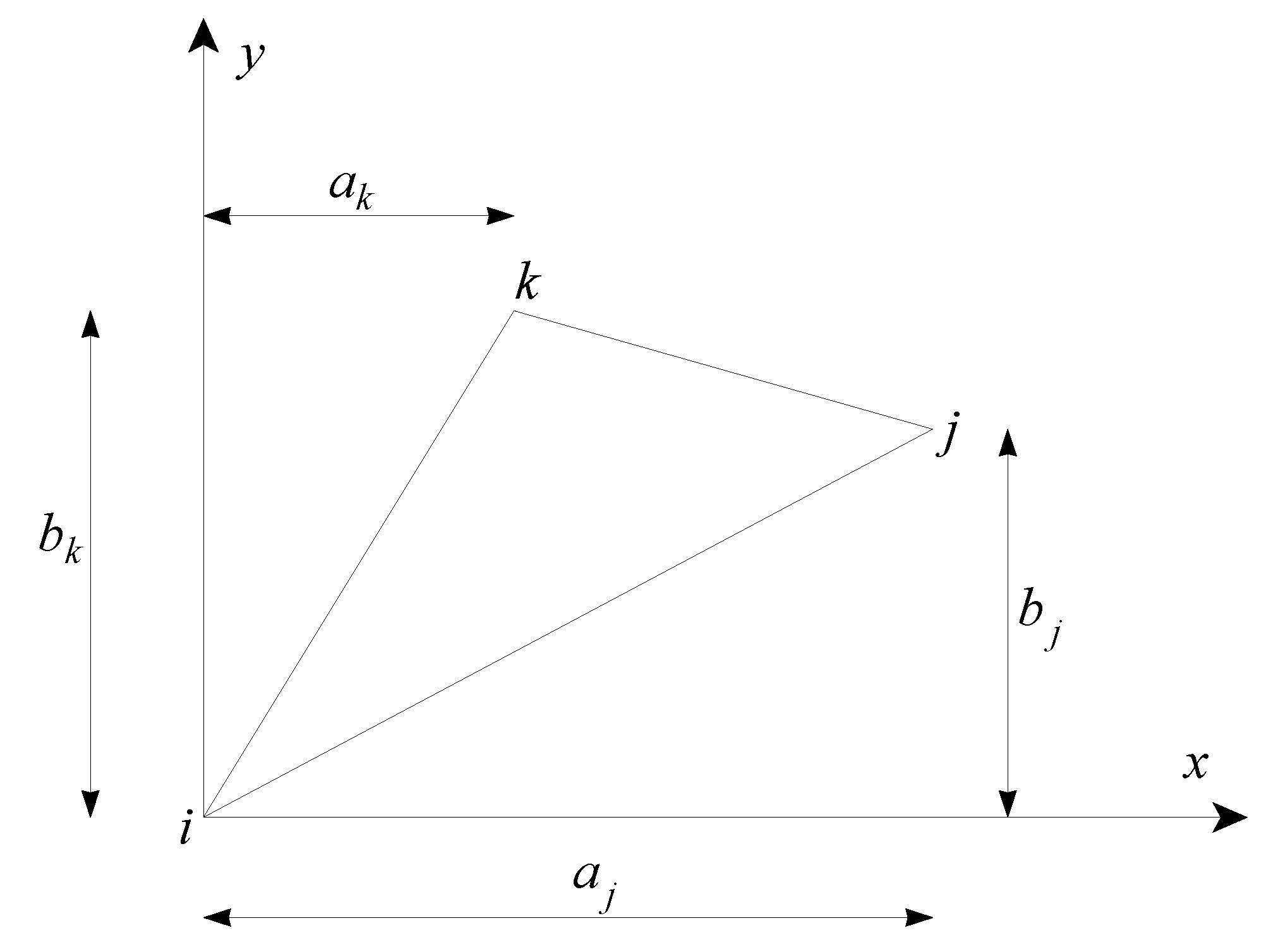
2. The Total Potential Energy of Plane Stress Members

As explained in the above paragraphs, the plates considered are divided into triangular elements such that the state variables are the displacements ui and vi at the nodes in x and y directions, respectively. Considering a linear variation in the displacements over the triangle, the displacement fields, such as u(x,y) and v(x,y), can be written as in Equations (1) and (2), respectively.
u ( x , y ) = u i + C 1 x + C 2 y ,
v ( x , y ) = v i + C 3 x + C 4 y ,
When the particular derivatives of displacement fields are taken with respect to x and y, the strains are expressed in terms of the constants C1, C2, C3, and C4.
ε x = u x = C 1 ,
ε y = v y = C 4 ,
γ = u y + v x = C 2 + C 3 ,
The strains εx, εy, and γ define the normal strain in x and y directions and the shear strain, respectively. If the coordinates of node i are the origin point, the nodal displacements of nodes i, j, and k can be expressed as follows, according to Figure 1:
u ( 0 , 0 ) = u i , v ( 0 , 0 ) = v i ,
u ( a j , b j ) = u j , v ( a j , b j ) = v j ,
u ( a k , b k ) = u k , v ( a k , b k ) = v k ,
By using Equations (1) and (2), the relations between the nodal displacements is written as Equation (9):
[ u j v j u k v k ] = [ a j b j 0 0 0 0 a j b j a k b k 0 0 0 0 a k b k ] [ C 1 C 2 C 3 C 4 ] + [ u i v i u i v i ] ,
The solution of Equation (9) yields the constants C1–C4 as in Equation (10)–(13):
C 1 = b k ( u j u i ) a j b k a k b j + b j ( u k u i ) a k b j a j b k ,
C 2 = a k ( u j u i ) a k b j a j b k + a j ( u k u i ) a j b k a k b j ,
C 3 = b k ( v j v i ) a j b k a k b j + b j ( v k v i ) a k b j a j b k ,
C 4 = a k ( v j v i ) a k b j a j b k + a j ( v k v i ) a j b k a k b j ,
The strain energy density that resulted due to deformation is written as Equation (14) for a two-dimensional elastic body:
e = ε = 0 ε σ d ε = 1 2 ( σ x ε x + σ y ε y + τ γ ) ,
When the solution of constants given as Equations (10)–(13) are used in Equations (3)–(5), the stains are written as follows:
ε x = b k ( u j u i ) a j b k a k b j + b j ( u k u i ) a k b j a j b k ,
ε y = a k ( v j v i ) a k b j a j b k + a j ( v k v i ) a j b k a k b j ,
γ = 1 a k b j a j b k + ( a k ( u j u i ) + a j ( u i u k ) + b k ( v i v j ) + b j ( v k v i ) ) ,
According to linear stress–strain relations for two-dimensional plane stress problems, stresses can be found from Equations (18)–(20), where E is the elasticity modulus and ν is the Poisson’s ratio:
σ x = E 1 ν 2 ( ε x + ν ε y ) ,
σ y = E 1 ν 2 ( ε y + ν ε x ) ,
τ = E 1 ν 2 ( 1 ν 2 γ ) ,
The substitution of Equations (15)–(17) to (18)–(20) yields Equations (21)–(23) for stresses for linear problems:
σ x = E ( ν 2 1 ) ( a k b j a j b k ) ν ( a k ( v i v j ) + a j ( v k v i ) ) + ( ν 1 ) ( b k ( u i u j ) b j ( u i u k ) ) ,
σ y = E ( ν 2 1 ) ( a k b j a j b k ) a k ( v i v j ) + a j ( v k v i ) + ν b k ( u j u i ) + ν b j ( u i u k ) ,
τ = E ( ν 2 1 ) ( a k b j a j b k ) ( 1 ν 2 a k ( u j u i ) + a j ( u i u k ) + b k ( v i v j ) + b j ( v k v i ) ,
Then, the strain energy for linear problems can be found from Equation (14), as can be seen in Equation (24), for one element:
e = E 4 ( 1 ν 2 ) ( a k b j a j b k ) 2 ( ( ν - 1 ) ( ( a k ( u j u i ) + a j ( u i u k ) + b k ( v i v j ) + b j ( v k v i ) ) 2 + 2 ( a k ( v j v i ) + a j ( v i v k ) ) ( ν ( a k ( v j v i ) + a j ( v i v k ) ) + b k ( u i u j ) + b j ( u k u i ) ) + 2 ( a k ( v j v i ) + a j ( v i v k ) ) ( a k ( v j v i ) + a j ( v i v k ) ) + ν b k ( u i u j ) + ν b j ( u k u i ) ) )
The strain energy density of the mth element (em) is multiplied with the volume (Vm) of the element to yield the strain energy of the mth element, as in Equation (25):
U i = e m V m ,
V m = ( a j b k a k b j ) t 2 ,
The volume is the multiplication of thickness (t) and area of the triangle element, as shown in Equation (26). The total strain energy of the system is calculated by adding the strain energy of all the elements. For the system consisting of n elements, the strain energy is as follows:
U = m = 1 n U m ,
In order to find the total potential energy (Πp), the work done by the external forces must be subtracted from the total strain energy. Equation (28) is given for a system with p number of nodes and point loads in x and y directions (Pxn and Pyn):
Π p = U n = 1 p ( P x n u n + P y n v n ) ,

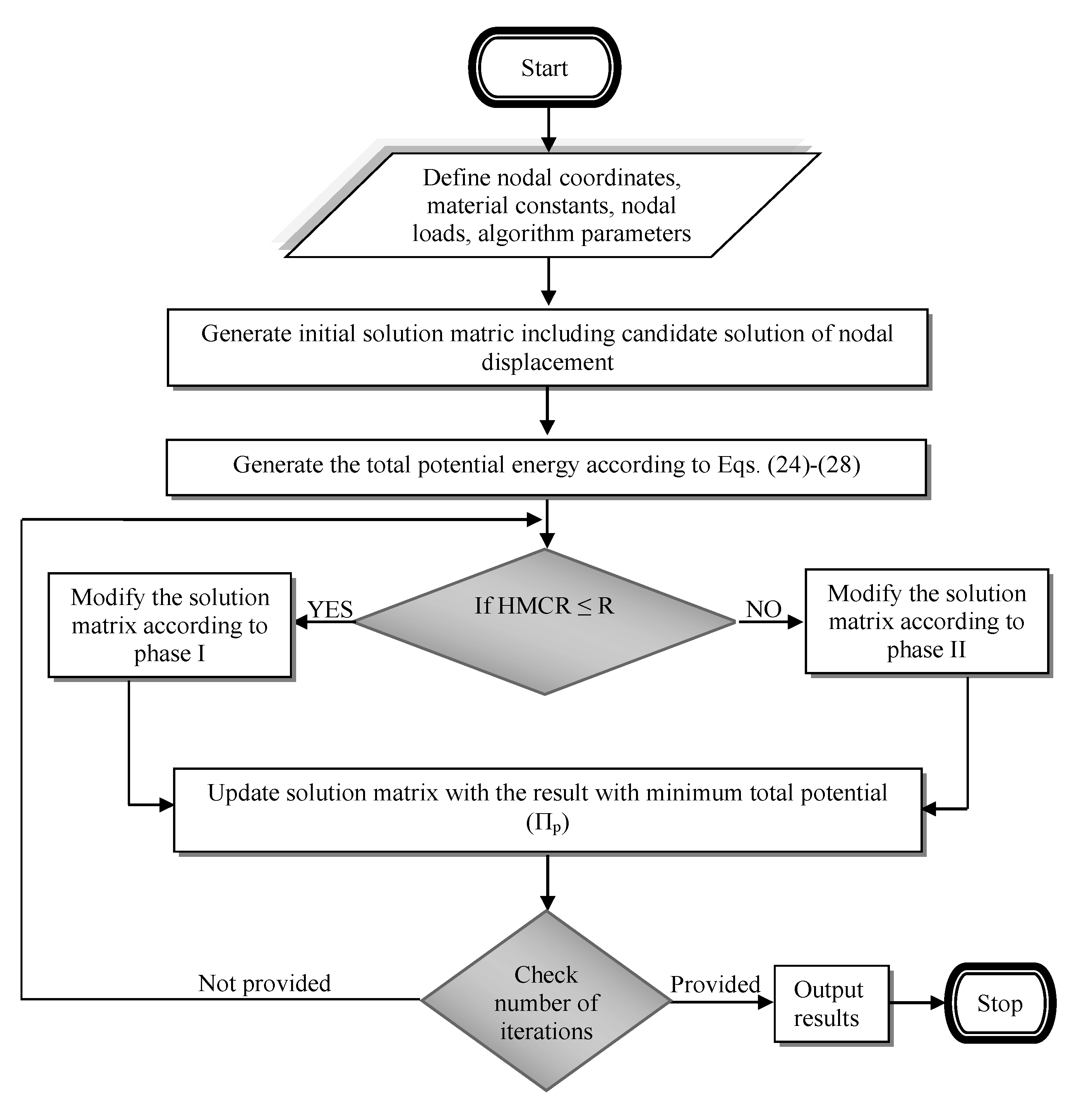
3. The Analysis Methodology

In TPO/MA, the nodal displacements (un and vn for m=1 to p) are assigned with candidate values according to the rules of employed metaheuristic algorithms. Each node has two nodal displacements and the number of design variables (s) is equal to two times the number of nodes (p) minus the number of fixed displacements (pf):
s = 2 p p f ,
The flowchart of the TPO/MA method for plane stress members is shown as Figure 2. The optimization process starts with the definition of the problem. Then, the nodal displacements must be assumed to find the total potential energy of the system. The initial solution matrix is generated via the candidate solutions of nodal displacements, and the assumed values are randomly chosen from the user-defined range of nodal displacements. Then, the iterative and essential optimization process starts, and special algorithm rules are taken into consideration for the maximum number of iterations.
In the methodology, there are two phases. Generally, one of these phases is global optimization, while the other one is a local optimization. These two phases are chosen via a parameter, and it is compared with a randomly generated number between 0 and 1 (R). The two phases of HS and HHS are chosen according to a parameter called the harmony memory considering rate (HMCR).
In this paper, the music inspired Harmony Search (HS) algorithm developed by Geem et al. [31] was employed and it was hybridized with the Flower Pollination Algorithm (FPA) developed by Yang [32]. The results of numerical examples were also compared with single forms of HS and the FPA, the Jaya Algorithm (JA) [33], and teaching–learning-based optimization (TLBO) [34].
After each iteration, the total potential energy values are calculated, and these values are compared with the existing values for updating.

3.1. Classical Harmony Search

In the classical form of HS, which has been applied to various structural optimization problems [35], the equation of the first phase is taken as Equation (30). This phase is the global search phase, which is also used for the generation of initial values.
X n e w = X min + r a n d ( 0 , 1 ) ( X max X min ) ,
In Equation (30), the maximum and minimum ranges of design variables are shown as Xmax and Xmin, respectively. A random number between 0 and 1 (ran (0,1)) is generated to form a new set of design variables (Xnew).
In local optimization phase of HS, a randomly selected existing solution (Xran) is used, and the neighborhood range (Xran ± fw) is scanned. The formulation of the local optimization of HS is shown as Equation (31):
X n e w = X r a n + f w ( 2 r a n d ( 0 , 1 ) 1 ) w i t h p r o b a b i l i t y o f P A R
The parameter “pitch adjusting rate (PAR)” is a parameter controlling the acceptable range around the chosen solution.

3.2. Hybridization of Harmony Search

To increase the convergence ability of the classical HS approach, the best existing solution can be used in global optimization. Moreover, using a distribution method that is not linear distribution may be effective. For that reason, a Lévy distribution can be used instead of considering a random number between 0 and 1. The Flower Pollination Algorithm (FPA) developed by Yang uses Lévy distribution and the best solution in the global pollination phase, which is generated via the observations biotic and cross pollinations. Due to the behavior of pollinators, such as insects, birds and other animals, a random flight (Lévy flight) is considered. The formulation of the global optimization phase of FPA and Hybrid Harmony Search (HHS) is given as Equation (32). According to the formulation, the existing solution (Xold) is modified according to best exiting solution (g*) and a Lévy distribution (L). Lévy distribution can be also assigned with random numbers covering a higher range than a linear distribution between 0 and 1. For that reason, it may affect the convergence ability negatively, but it will prevent to track to a local optimum result which is a close value to currently existing best solution that is not the global optimum.
X n e w = X o l d + L ( g * X o l d ) ,

4. Numerical Examples

As numerical examples, three problems were solved, and all solutions were compared with the finite element method (FEM) results. For all problems, the Harmony memory considering rate (HMCR) was taken as 0.5, while PAR is equal to 0.1. These parameters are the best cases for the examples in the study for sensitive final solutions and fast convergence. The HMCR value as 0.5 leads to usage of global and local optimization phases with equal probability, and the PAR value as 0.1 is a suitable value for convergence around existing solutions.

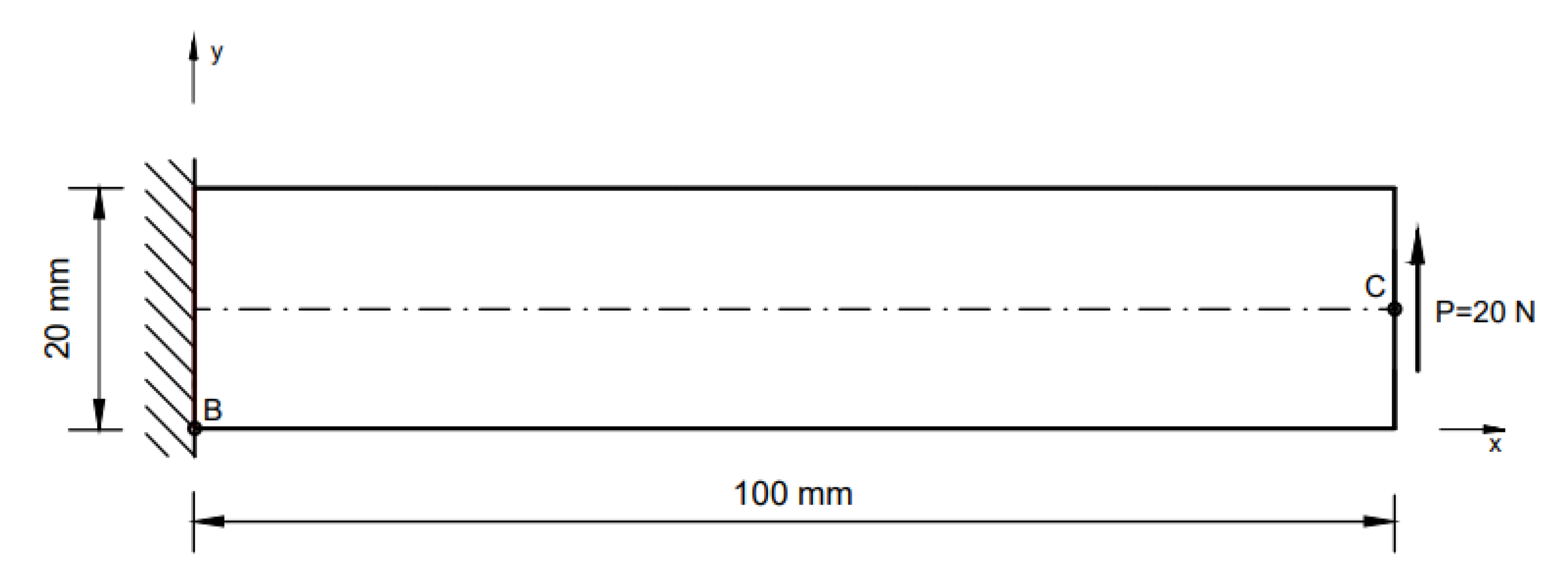
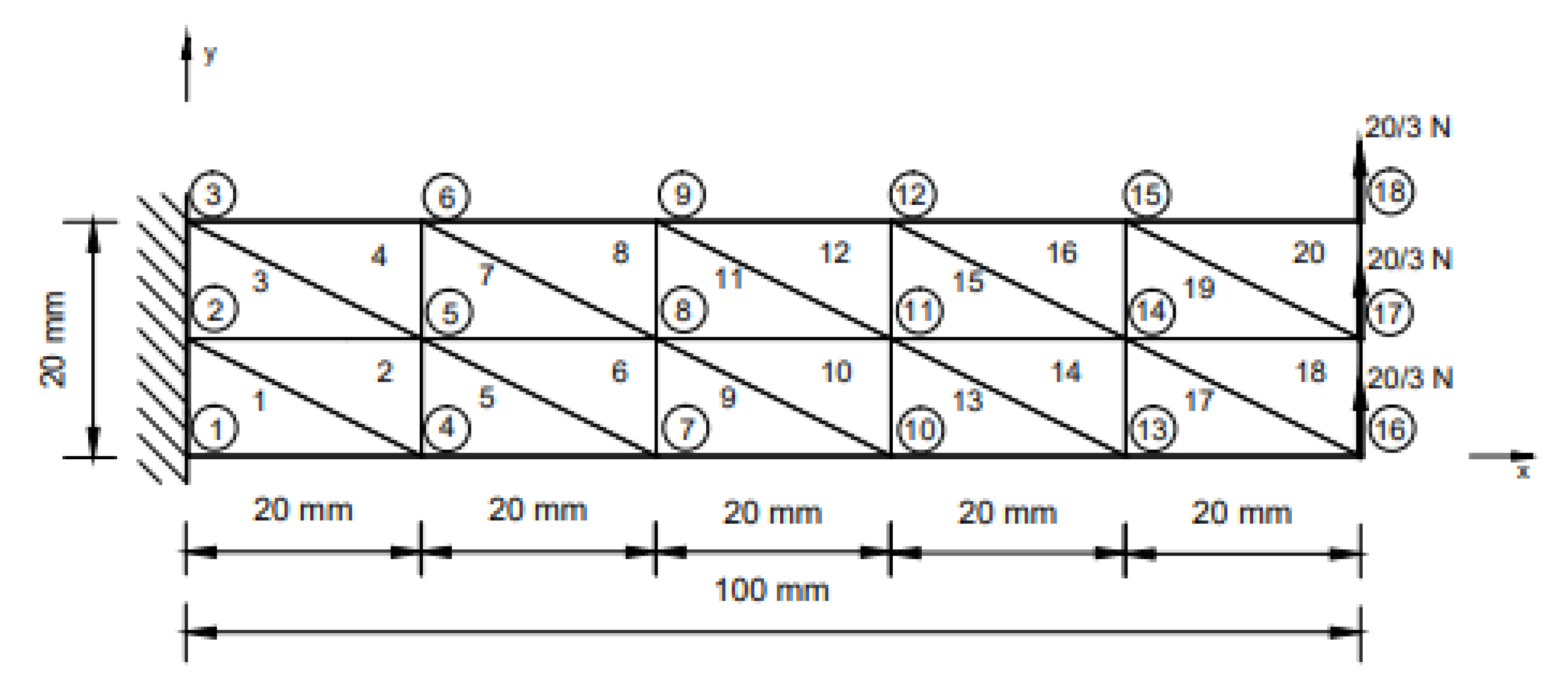
4.1. Structure 1: Cantilever Beam Under a Concentered Load

The figure of the first structure, which was previously considered by Cook [36,37], is given as Figure 3. The cantilever beam is loaded at the end (point C) in +y direction and the intensity of the load P is 20 N. The elasticity modulus and Poisson ratio of the material of the beam are 100 N/mm2 and 0.3, respectively. The thickness of the members is 10 mm. The triangulation prepared for the analyses can be seen in the Figure 4.
The cantilever beam has 15 free nodes and 30 displacement values considered as design variables. As seen in the results presented in Table 1, TPO/MA using HHS, FPA, JA, and TLBO has similar solutions to FEM. Application with HS resulted in a total potential energy value close to the others, but the nodal displacements have important differences, as compared to other algorithms. On the other hand, HS needs more iterations than other methods; this makes it computationally ineffective for the problem.
The single-phase JA has a better convergence rate as a classical form algorithm since it reached at minimum energy at 672375th iteration, while the others were found nearly at the end of 106 iterations. HHS has a significantly better convergence ability than JA by finding the best solution with 531810 iterations. By using HSS, all failures of HS are prevented.

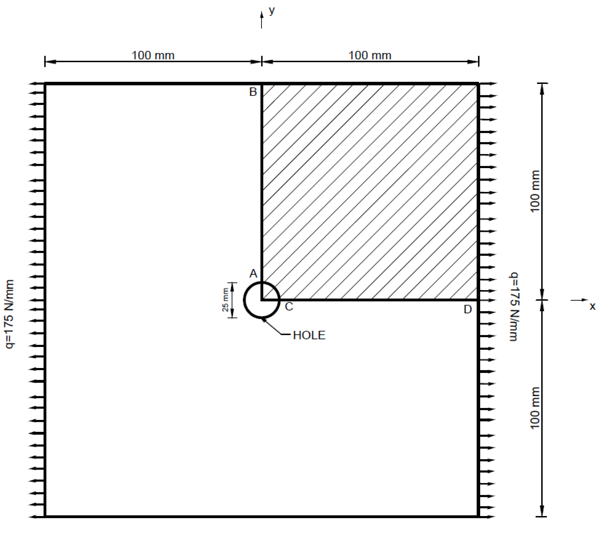
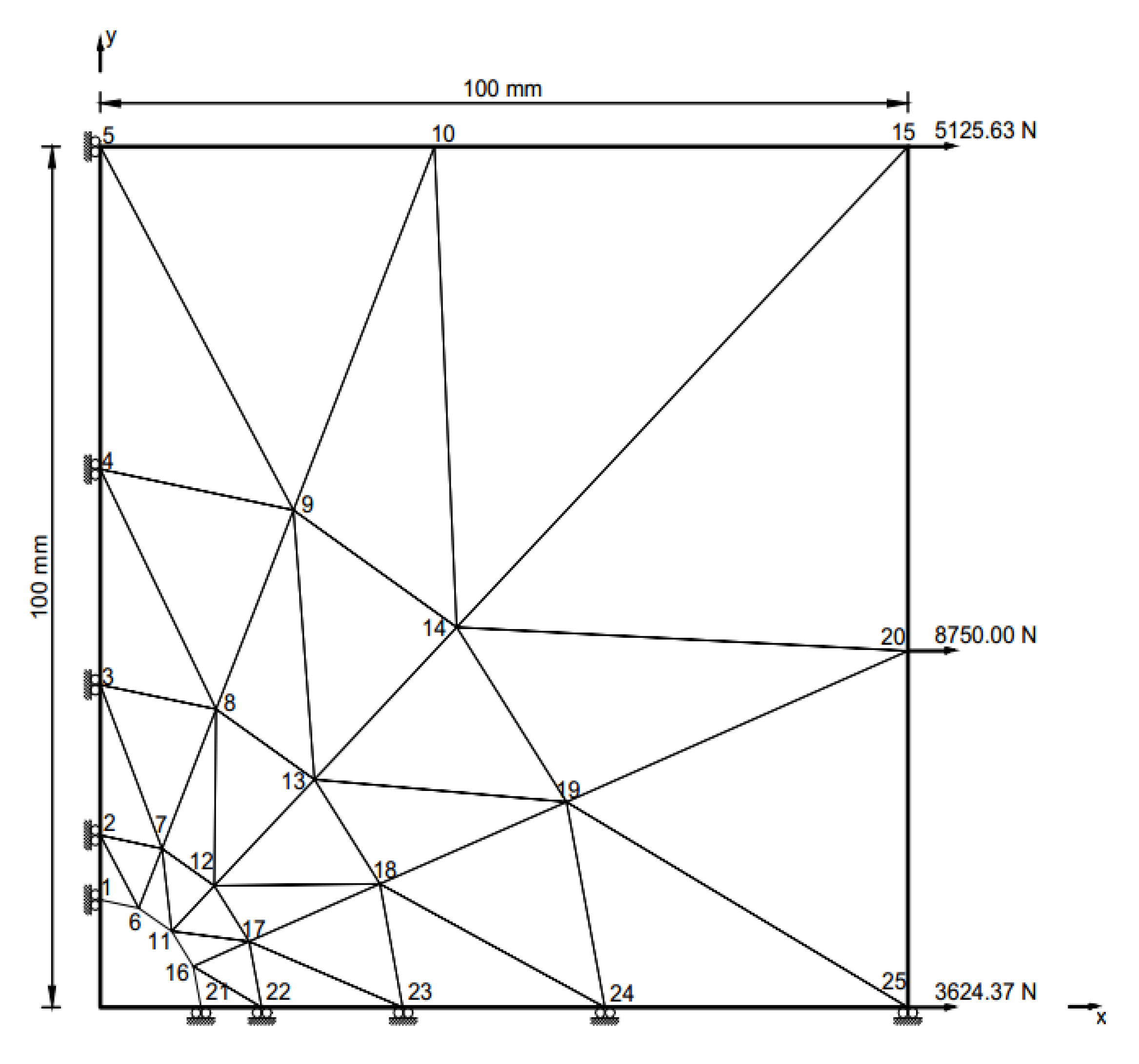
4.2. Structure 2. A Plate with the Hole in the Middle (32 Members-25 Nodes)

The second structure is the plate with the hole in the middle [37,38], having a thickness of 2.5 mm (Figure 5). The material is characterized by the elasticity modulus 70000 N/mm2 and Poisson ratio 0.3. The uniformly distributed load (q) with a density of 175 N/mm is applied to the plate in x direction. Because of symmetry, the quarter system shown in Figure 6 with 32 members and 25 nodes was solved.
The number of design variables is 40 because of the 10 fixed displacements of the 50 nodal displacements. The solutions of the design variables are shown in Table 2 for FPA, JA, HS, HHS, and TLBO. Similar to Structure 1, HHS, FPA, JA, and TLBO have the same results with FEM, while HS is close to the solutions. The number of analyses to find the minimum energy is close to each other for all methods except HHS. In this example, one cannot make a distinction among the classical form algorithms applied to their accuracy, speed, and robustness, although the number of state variables becomes increased from 30 to 40 as compared to 1st example. HSS also has a fast-computational ability comparing to all other algorithms.

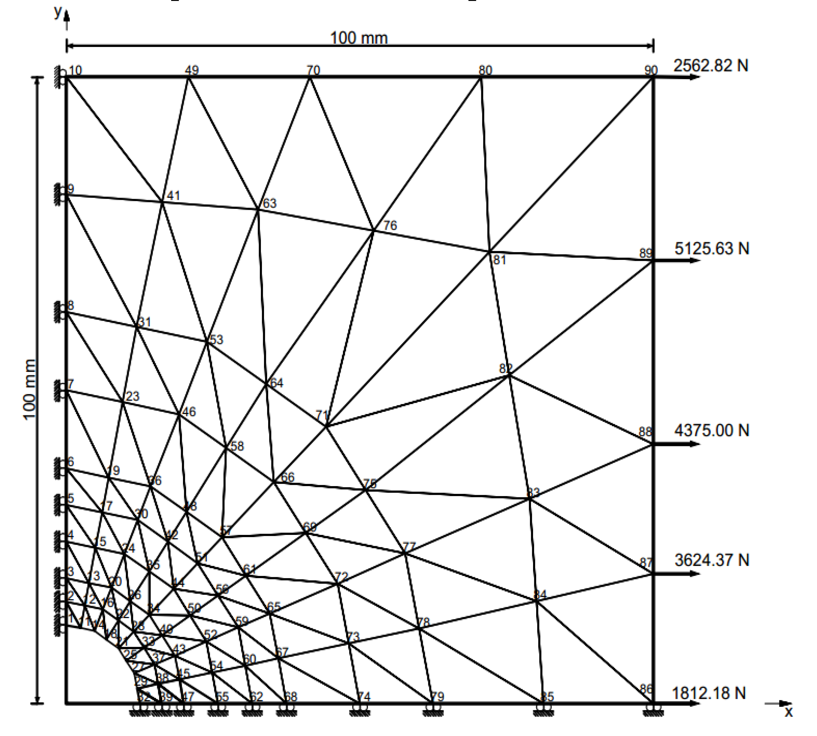
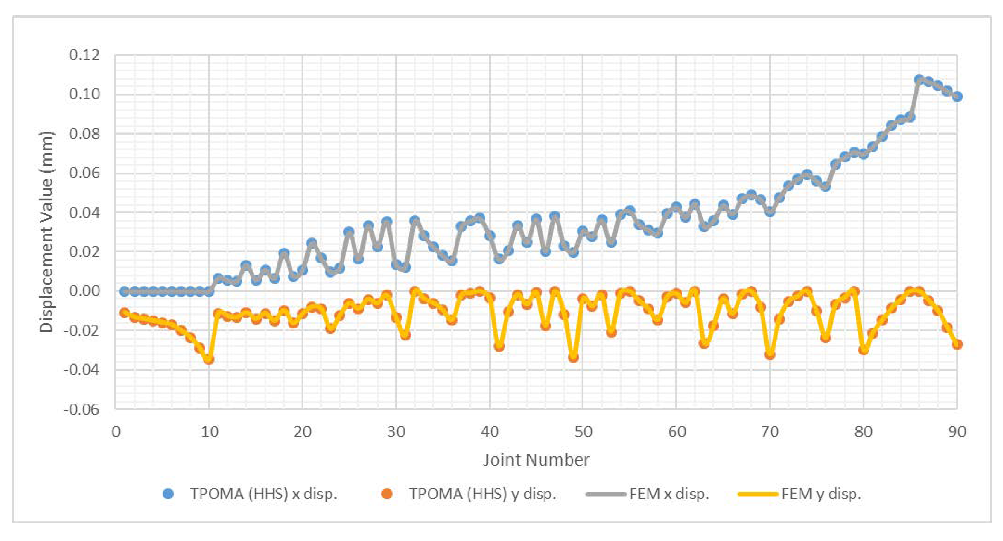
4.3. Structure 3. A Plate with a Hole in the Middle (144 Members and 90 Nodes)

The plate presented as Structure 2 is also investigated with a different meshing option, as seen in Figure 7, in order to find a deflected form of the system for more points on the plane. Furthermore, by considering more members, an analysis result close to the exact solution can also be found. In that case, the total potential energy and the displacement values for this example will be different to the results of Structure 2. The minimum energy and the analysis number needed for the minimum value are given as Table 3. All nodal displacements are plotted in Figure 8 for FEM and HHS results. Similar conclusions can be drawn in this example as compared to the first two problems solved.

5. Conclusions and Future Studies

The main purpose of this study is to see the applicability of the method called TPO/MA to more general structures than those it was previously applied to. In fact, TPO/MA has been applied until now to trusses and truss-like structures as cables and tensegric structures. The current study has shown that plates can be also analyzed using TPO/MA.
According to the No-Free-Lunch theorem [39], an algorithm may outperform another one in an example, while another one outperforms that algorithm in a second example. For that reason, several metaheuristic algorithms, such as HS, FPA, TLBO, and JA, were tested with the proposed novel hybrid method in the study. While HS has slightly failed to find the minimum energy level, the proposed HHS reached to minimum energy level quickly than the other algorithms. The methodology using HSS is effective on TPO/MA on solving plane stress problems. The processing time of the all iterations is in an acceptable value. By using TPO/MA, 1000 iterations of three examples were solved in 1.5 s, 2.5 s, and 8 s, respectively. Compared to other approaches, HHS can nearly find the global optimum results by half and 1/3 of the number of function evaluations for the first two examples and third example, respectively.
The analysis results found according to the HHS approach is effective to find the same results with the FEM method. Only minor differences (last than 1%) can be seen, but the total potential energy values are not affected.
Based on these considerations, it can be easily foreseen that this study will be followed by applications of TPO/MA on plane strain problems, plates with three-dimensional deformations, those with nonlinear constitutive equations, and those with other nonlinearities.

Author Contributions

A.E.K. and G.B. generated the analyses codes. Y.C.T. developed theory background and formulations of the methodology. The text of paper was formed by S.M.N., Y.C.T. and M.Y.. The figures were drawn by A.E.K. and M.Y., Z.W.G. supervised the research direction. All authors have read and approved the final manuscript.

Funding

This research was supported by the Energy Cloud R&D Program through the National Research Foundation of Korea (NRF) funded by the Ministry of Science, ICT (2019M3F2A1073164).

Conflicts of Interest

The authors declare no conflict of interest.

References

  1. Levy, R.; Spillers, W.R. Analysis of Geometrically Nonlinear Structures, 2nd ed.; Kluwer Academic Publishers: Dordtrecht, The Netherlands, 2003. [Google Scholar]
  2. Saffari, H.; Fadaee, M.J.; Tabatabaei, R. Nonlinear analysis of space trusses using modified normal flow algorithm. J. Struct. Eng. 2008, 134, 998–1005. [Google Scholar] [CrossRef]
  3. Krenk, S. Non-linear Modeling and Analysis of Solids and Structures; Cambridge University Press: Cambridge, UK, 2009. [Google Scholar]
  4. Greco, M.; Menin, R.C.G.; Ferreira, I.P.; Barros, F.B. Comparison between two geometrical nonlinear methods for truss analyses. Struct. Eng. Mech. 2012, 41, 735–750. [Google Scholar] [CrossRef]
  5. Nazir, A.; Abate, K.M.; Kumar, A.; Jeng, J.Y. A state-of-the-art review on types, design, optimization, and additive manufacturing of cellular structures. Int. J. Adv. Manuf. Technol. 2019, 104, 3489–3510. [Google Scholar] [CrossRef]
  6. Toklu, Y.C. Nonlinear analysis of trusses through energy minimization. Comput. Struct. 2004, 82, 1581–1589. [Google Scholar] [CrossRef]
  7. Toklu, Y.C.; Bekdas, G.; Temur, R. Analysis of trusses by total potential optimization method coupled with harmony search. Struct. Eng. Mech. 2013, 45, 183–199. [Google Scholar] [CrossRef]
  8. Temür, R.; Türkan, Y.; Toklu, Y. Geometrically Nonlinear Analysis of Trusses Using Particle Swarm Optimization; Springer International Publishing: Basel, Switzerland, 2015. [Google Scholar]
  9. Toklu, Y.C.; Temur, R.; Bekdaş, G. Computation of non-unique solutions for trusses undergoing large deflections. Int. J. Comput. Methods 2015, 12, 1550022. [Google Scholar] [CrossRef]
  10. Temür, R.; Bekdaş, G.; Toklu, Y.C. Total potential energy minimization method in structural analysis considering material nonlinearity. Chall. J. Struct. Mech. 2017, 3, 129–133. [Google Scholar] [CrossRef]
  11. Toklu, Y.C.; Uzun, F. Analysis of tensegric structures by total potential optimization using metaheuristic algorithms. J. Aerosp. Eng. 2016, 29, 04016023. [Google Scholar] [CrossRef]
  12. Toklu, Y.C.; Bekdaş, G.; Temur, R. Analysis of cable structures through energy minimization. Struct. Eng. Mech. 2017, 62, 749–758. [Google Scholar]
  13. Bekdas, G.; Kayabekir, A.E.; Niğdeli, S.M.; Toklu, Y.C. Advanced energy based analyses of trusses employing hybrid metaheuristics. Struct. Des. Tall Spec. Build. 2019, 28, e1609. [Google Scholar] [CrossRef]
  14. Lee, K.S.; Geem, Z.W. A new structural optimization method based on the harmony search algorithm. Comput. Struct. 2004, 82, 781–798. [Google Scholar] [CrossRef]
  15. Lee, K.S.; Geem, Z.W.; Lee, S.H.; Bae, K.W. The harmony search heuristic algorithm for discrete structural optimization. Eng. Optim. 2005, 37, 663–684. [Google Scholar] [CrossRef]
  16. Kaveh, A.; Talatahari, S. Particle swarm optimizer, ant colony strategy and harmony search scheme hybridized for optimization of truss structures. Comput. Struct. 2009, 87, 267–283. [Google Scholar] [CrossRef]
  17. Hasançebi, O.; Erdal, F.; Saka, M.P. Adaptive harmony search method for structural optimization. J. Struct. Eng. 2010, 136, 419–431. [Google Scholar] [CrossRef]
  18. Martini, K. Harmony search method for multimodal size, shape, and topology optimization of structural frameworks. J. Struct. Eng. 2011, 137, 1332–1339. [Google Scholar] [CrossRef] [Green Version]
  19. Degertekin, S.O. Improved harmony search algorithms for sizing optimization of truss structures. Comput. Struct. 2012, 92, 229–241. [Google Scholar] [CrossRef]
  20. Gholizadeh, S.; Barzegar, A. Shape optimization of structures for frequency constraints by sequential harmony search algorithm. Eng. Optim. 2013, 45, 627–646. [Google Scholar] [CrossRef]
  21. Amini, F.; Ghaderi, P. Hybridization of harmony search and ant colony optimization for optimal locating of structural dampers. Appl. Soft Comput. 2013, 13, 2272–2280. [Google Scholar] [CrossRef]
  22. Bekdaş, G.; Nigdeli, S.M. Estimating optimum parameters of tuned mass dampers using harmony search. Eng. Struct. 2011, 33, 2716–2723. [Google Scholar] [CrossRef]
  23. Nigdeli, S.M.; Bekdaş, G. Optimum tuned mass damper design in frequency domain for structures. KSCE J. Civ. Eng. 2017, 21, 912–922. [Google Scholar] [CrossRef]
  24. Nigdeli, S.M.; Bekdaş, G.; Alhan, C. Optimization of seismic isolation systems via harmony search. Eng. Optim. 2014, 46, 1553–1569. [Google Scholar] [CrossRef]
  25. Jin, H.; Xia, J.; Wang, Y.Q. Optimal sensor placement for space modal identification of crane structures based on an improved harmony search algorithm. J. Zhejiang Univ.-Sci. A 2015, 16, 464–477. [Google Scholar] [CrossRef] [Green Version]
  26. Mashayekhi, M.; Salajegheh, E.; Dehghani, M. Topology optimization of double and triple layer grid structures using a modified gravitational harmony search algorithm with efficient member grouping strategy. Comput. Struct. 2016, 172, 40–58. [Google Scholar] [CrossRef]
  27. Kazemi, E.N.; Shabakhty, N.; Abbasi, K.M.; Sanayee, M.S. Structural reliability: An assessment using a new and efficient two-phase method based on artificial neural network and a harmony search algorithm. Civ. Eng. Infrastruct. J. 2016, 49, 1–20. [Google Scholar]
  28. Daloglu, A.T.; Artar, M.; Ozgan, K.; Karakas, A.I. Optimum design of braced steel space frames including soil-structure interaction via teaching-learning-based optimization and harmony search algorithms. Adv. Civ. Eng. 2018, 2018, 3854620. [Google Scholar] [CrossRef] [Green Version]
  29. de Almeida, F.S. Optimization of laminated composite structures using harmony search algorithm. Compos. Struct. 2019, 221, 110852. [Google Scholar] [CrossRef] [Green Version]
  30. Zhang, T.; Geem, Z.W. Review of harmony search with respect to algorithm structure. Swarm Evolutionary Comput. 2019, 48, 31–43. [Google Scholar] [CrossRef]
  31. Geem, Z.W.; Kim, J.H.; Loganathan, G.V. A new heuristic optimization algorithm: Harmony search. Simulation 2001, 76, 60–68. [Google Scholar] [CrossRef]
  32. Yang, X.S. Flower pollination algorithm for global optimization. In Proceedings of the Unconventional Computation and Natural Computation 2012, Orléans, France, 3–7 September 2012; pp. 240–249. [Google Scholar]
  33. Rao, R. Jaya: A simple and new optimization algorithm for solving constrained and unconstrained optimization problems. Int. J. Ind. Eng. Comput. 2016, 7, 19–34. [Google Scholar]
  34. Rao, R.V.; Savsani, V.J.; Vakharia, D.P. Teaching–learning-based optimization: A novel method for constrained mechanical design optimization problems. Comput.-Aided Des. 2011, 43, 303–315. [Google Scholar] [CrossRef]
  35. Saka, M.P.; Hasançebi, O.; Geem, Z.W. Metaheuristics in structural optimization and discussions on harmony search algorithm. Swarm Evol. Comput. 2016, 28, 88–97. [Google Scholar] [CrossRef]
  36. Cook, R.D. Finite Element Modelling for Stress Analysis; John Wiley &Sons, Inc.: Hoboken, NJ, USA, 1995; ISBN 0-471-10774-3. [Google Scholar]
  37. Gazi, H. Sonlu Elemanlar Yönemi ile Çalışan Bir Bilgisayar Programının Geliştirilmesi ve Düzlem Gerilme —Düzlem Deformasyon Problemlerinin Analizi. MSc Thesis, Istanbul University, Istanbul, Turkey, 2008. [Google Scholar]
  38. Weawer, W.; Johnston, P.R. Finite Element for Structural Analysis; Prentice—Hall, Inc.: Upper Saddle River, NJ, USA, 1984. [Google Scholar]
  39. Wolpert, D.H.; Macready, W.G. No free lunch theorems for optimization. IEEE Trans. Evol. Comput. 1997, 1, 67–82. [Google Scholar] [CrossRef] [Green Version]
Figure 1. The triangular element.
Applsci 10 02301 g001
Figure 2. The flowchart of the total potential optimization using metaheuristic algorithms (TPO/MA).
Applsci 10 02301 g002
Figure 3. Structure 1: Cantilever beam.
Applsci 10 02301 g003
Figure 4. Mathematical model prepared for the analyses of the cantilever beam.
Applsci 10 02301 g004
Figure 5. Structure 2: A plate with the hole in the middle.
Applsci 10 02301 g005
Figure 6. Mathematical models with 32 members and 25 nodes.
Applsci 10 02301 g006
Figure 7. Structure 2: A plate with the hole in the middle.
Applsci 10 02301 g007
Figure 8. Nodal displacements for Structure 3.
Applsci 10 02301 g008
Table 1. Solutions for the cantilever beam with 20 plane members
TPOMA (FPA)TPOMA (JA)TPOMA (HS)TPOMA (HHS)TPOMA (TLBO)FEM
NodeΔx (mm)Δy (mm)Δx (mm)Δy (mm)Δx (mm)Δy (mm)Δx (mm)Δy (mm)Δx (mm)Δy (mm)Δx (mm)Δy (mm)
40.193690.251510.193690.251510.207150.270890.192590.249920.193690.251510.19370.2515
50.000590.241760.000590.24176−0.000030.260780.000590.240220.000590.241760.00060.2418
6−0.199120.25858−0.199120.25858−0.213260.27713−0.197990.25693−0.199120.25858−0.19910.2586
70.347010.848140.347010.848140.369920.907090.345170.843170.347010.848140.3470.8481
8−0.003140.8425−0.003140.8425−0.00460.90067−0.003120.83754−0.003140.8425−0.00310.8425
9−0.354080.85627−0.354080.85627−0.379170.91413−0.352200.85123−0.354080.85627−0.35410.8563
100.45471.709670.45471.709670.485811.830840.452471.700250.45471.709670.45471.7097
11−0.005761.70704−0.005761.70704−0.006861.82991−0.005711.69762−0.005761.70704−0.00581.707
12−0.466191.71762−0.466191.71762−0.501551.8422−0.463881.70816−0.466191.71762−0.46621.7176
130.518582.746960.518582.746960.550032.939250.516182.732580.518582.746960.51862.747
14−0.00842.74754−0.00842.74754−0.010112.94063−0.008342.73315−0.00842.74754−0.00842.7475
15−0.534222.75474−0.534222.75473−0.570022.94848−0.531722.74033−0.534222.75473−0.53422.7547
160.538613.874280.538613.874280.571924.138810.536193.854870.538613.874280.53863.8743
17−0.010543.87495−0.010543.87495−0.012744.14002−0.010483.85555−0.010543.87495−0.01053.8749
18−0.559393.88219−0.559393.88219−0.594124.14664−0.556863.86278−0.559393.88219−0.55943.8822
Пp (Nmm)−38.8−38.8−38.6−38.8−38.8−38.8
Analysis number999103672375999343531810987341
Table 2. Solutions for the plate with the hole in the middle with 32 members.
TPOMA (FPA)TPOMA (JA)TPOMA (HS)TPOMA (HHS)TPOMA (TLBO)FEM
NodeΔx (mm)Δy (mm)Δx (mm)Δy (mm)Δx (mm)Δy (mm)Δx (mm)Δy (mm)Δx (mm)Δy (mm)Δx (mm)Δy (mm)
10.000000−0.0067290.000000−0.0067290.000000−0.0062680.000000−0.0067290.000000−0.0067290.000000−0.006729
20.000000−0.0105090.000000−0.0105090.000000−0.0100430.000000−0.0105090.000000−0.0105090.000000−0.010509
30.000000−0.0148990.000000−0.0148990.000000−0.0148020.000000−0.0148990.000000−0.0148990.000000−0.014899
40.000000−0.0217820.000000−0.0217820.000000−0.0217990.000000−0.0217820.000000−0.0217820.000000−0.021782
50.000000−0.0330780.000000−0.0330780.000000−0.0329400.000000−0.0330780.000000−0.0330780.000000−0.033078
60.010933−0.0076550.010933−0.0076550.010747−0.0072950.010933−0.0076550.010933−0.0076550.010933−0.007655
70.010157−0.0089010.010157−0.0089010.010037−0.0086700.010157−0.0089010.010157−0.0089010.010157−0.008901
80.015549−0.0128420.015549−0.0128420.015359−0.0126510.015549−0.0128420.015549−0.0128420.015549−0.012842
90.024757−0.0194300.024757−0.0194300.024694−0.0192000.024757−0.0194300.024757−0.0194300.024757−0.019430
100.040879−0.0312240.040879−0.0312240.041076−0.0311810.040879−0.0312240.040879−0.0312240.040879−0.031224
110.020164−0.0054160.020164−0.0054160.019642−0.0052100.020164−0.0054160.020164−0.0054160.020164−0.005416
120.020301−0.0048720.020301−0.0048720.019816−0.0048090.020301−0.0048720.020301−0.0048720.020301−0.004872
130.030207−0.0083080.030207−0.0083080.029842−0.0081500.030207−0.0083080.030207−0.0083080.030207−0.008308
140.046860−0.0136320.046860−0.0136320.046616−0.0135800.046860−0.0136320.046860−0.0136320.046860−0.013632
150.100048−0.0282300.100048−0.0282300.100091−0.0285510.100048−0.0282300.100048−0.0282300.100048−0.028230
160.028501−0.0026510.028501−0.0026510.028253−0.0025730.028501−0.0026510.028501−0.0026510.028501−0.002651
170.029659−0.0015860.029659−0.0015860.029287−0.0015120.029659−0.0015860.029659−0.0015860.029659−0.001586
180.041562−0.0036150.041562−0.0036150.041091−0.0035370.041562−0.0036150.041562−0.0036150.041562−0.003615
190.062858−0.0066780.062858−0.0066780.062583−0.0066490.062858−0.0066780.062858−0.0066780.062858−0.006678
200.103448−0.0106290.103448−0.0106290.103312−0.0109190.103448−0.0106290.103448−0.0106290.103448−0.010629
210.0306750.0000000.0306750.0000000.0303600.0000000.0306750.0000000.0306750.0000000.0306750.000000
220.0336620.0000000.0336620.0000000.0332200.0000000.0336620.0000000.0336620.0000000.0336620.000000
230.0460970.0000000.0460970.0000000.0455170.0000000.0460970.0000000.0460970.0000000.0460970.000000
240.0687700.0000000.0687700.0000000.0682950.0000000.0687700.0000000.0687700.0000000.0687700.000000
250.1054910.0000000.1054910.0000000.1050300.0000000.1054910.0000000.1054910.0000000.1054910.000000
Пp (Nmm)−900.16−900.16−900.08−900.16−900.16−900.16
Analysis number5902563115591462999756575
Table 3. Total potential energy results for the system with 144 members.
TPOMA (FPA)TPOMA (JA)TPOMA (HS)TPOMA (HHS)TPOMA (TLBO)FEM
Пp (Nmm)−905.08−905.08−901.48−905.08−905.08−905.08
Analysis number999992972853876457269416947564

