Article

An Improved Novel Global Harmony Search Algorithm Based on Selective Acceptance

1
Business School, University of Shanghai for Science and Technology, Shanghai 200093, China
2
School of Intelligent Manufacturing, Panzhihua University, Panzhihua 617000, China
*
Author to whom correspondence should be addressed.
Appl. Sci. 2020, 10(6), 1910; https://doi.org/10.3390/app10061910
Submission received: 6 February 2020 / Revised: 5 March 2020 / Accepted: 6 March 2020 / Published: 11 March 2020

Abstract

:
The novel global harmony search (NGHS) algorithm is proposed in 2010, and it is an improved harmony search (HS) algorithm which combines the particle swarm optimization (PSO) and the genetic algorithm (GA). One of the main differences between the HS and NGHS algorithms is that of using different mechanisms to renew the harmony memory (HM). In the HS algorithm, in each iteration, the new harmony is accepted and replaced the worst harmony in the HM while the fitness of the new harmony is better than the worst harmony in the HM. Conversely, in the NGHS algorithm, the new harmony replaces the worst harmony in the HM without any precondition. However, in addition to these two mechanisms, there is one old mechanism, the selective acceptance mechanism, which is used in the simulated annealing (SA) algorithm. Therefore, in this paper, we proposed the selective acceptance novel global harmony search (SANGHS) algorithm which combines the NGHS algorithm with a selective acceptance mechanism. The advantage of the SANGHS algorithm is that it balances the global exploration and local exploitation ability. Moreover, to verify the search ability of the SANGHS algorithm, we used the SANGHS algorithm in ten well-known benchmark continuous optimization problems and two engineering problems and compared the experimental results with other metaheuristic algorithms. The experimental results show that the SANGHS algorithm has better search ability than the other four harmony search algorithms in ten continuous optimization problems. In addition, in two engineering problems, the SANGHS algorithm also provided a competition solution compared with other state-of-the-art metaheuristic algorithms.

1. Introduction

In the past two decades, the interest in the research related to metaheuristic algorithms has increased significantly due to the fact that existing numerical methods do not allow for solving a number of complex optimization problems, such as discrete structural optimization [1], design of water distribution networks [2], and vehicle routing [3]. A metaheuristic algorithm is applied to simulate the randomness and rules in natural phenomena. For example, the genetic algorithm (GA) [4] imitates the process of the biological evolutionary and natural selection. The particle swarm optimization (PSO) [5] was inspired by the animal behavior, namely, the foraging behavior of bird flocking. In addition, there are many algorithms extending PSO and GA, such as the harmony search (HS) algorithm [6] and the honey bee mating optimization (HBMO) [7]. These algorithms have proved their ability to search for better solutions than numerical methods in extensive optimization problems [8,9,10]. However, compared with theses algorithms, the HS algorithm which imitates an improvisation process of a harmony has two features. Firstly, it has fewer mathematical requirements and is easy to implement. Secondly, each decision variable in a new solution vector could be generated independently by considering all of the existing solution vectors [11]. Due to these two features, the HS algorithm has stronger adaptability for many engineering problems and could generate competition results compared with the GA [11]. In addition, based on the above advantages, many modified versions of the HS algorithm are proposed to further improve the searching ability of the HS algorithm, such as the improved harmony search (IHS) algorithm [11], the self-adaptive global best harmony search (SGHS) algorithm [12], and the novel global harmony search (NGHS) algorithm [13]. These modified versions of the HS algorithm have better search ability than the original HS algorithm.
It is worth noting that, among these HS algorithms, the mechanism that is used to decide whether a new generated harmony (solution vector) is accepted and replaces the worst harmony in the harmony memory (HM) or not is different. The HM is a storage of the harmony. Specifically, the HS, IHS, and SGHS algorithms accept a new generated harmony only when it is better than the worst harmony in the current HM. This mechanism, we call it accept-the-better-only mechanism, reminded us of the tabu search (TS) algorithm [14] which also only accepts the better solution vector in the searching process. Conversely, in the NGHS algorithm, a new generated harmony is accepted and replaced the worst harmony in the HM without preconditions in each iteration. This mechanism, we call it accept-everything mechanism, is the same one used in the PSO and GA. In the PSO algorithm, in each iteration, after calculating the velocity of the particle, the particle will fly to the new position according to its velocity whether the fitness of the new position is better than the current position or not. However, while we were discussing these two acceptance mechanisms, we suddenly came up with an old algorithm, the simulated annealing (SA) algorithm [15]. In the SA algorithm, in each iteration, the new solution vector is accepted or not according to the acceptable probability (AP), which is calculated by the Boltzmann distribution. Thus, the SA algorithm inspired us to investigate whether the AP affects the search ability or not in the NGHS algorithm. Therefore, in this paper, we proposed the selective acceptance novel global harmony search (SANGHS) algorithm, which combined the selective acceptance mechanism with the NGHS algorithm. Moreover, we proposed a proportion formula to calculate the AP according to the convergence degree. To verify the searching performance of the SANGHS algorithm, we used the SANGHS algorithms in ten well-known optimization problems and two engineering problems and compared the experimental results with other 15 algorithms. The results revealed that the SANGHS algorithm outperformed other 15 algorithms.
The remainder of this paper is organized as follows. In Section 2, the HS, IHS, SGHS, and the NGHS algorithms are introduced. Section 3 describes the SANGHS algorithm. A considerable number of experiments were conducted to test the search ability of the proposed SANGHS algorithm, and the corresponding experiments results are analyzed in Section 4. Conclusions and future research directions are provided in Section 5.

2. HS, IHS, SGHS, and NGHS Algorithms

2.1. Harmony Search Algorithm

The harmony search was proposed by Geem in 2001 [6]. Unlike other metaheuristic algorithms used to simulate the reproductive or foraging processes in the biological world, such as PSO and GA, the harmony search algorithm is inspired by a jazz trio and simulates its improvisation process [6]. The HS algorithm introduces musical notes to represent decision variables in practical problems. The number of musical notes is determined by the number of decision variables. Each note is played by a musician. Harmony requires two or more notes to be played at the same time. Thereby, each harmony represents a set of decision values. The HS algorithm simulates this in an improvisation process; hence, if the new harmony is better than the worst harmony, the new harmony will be saved to the harmony memory, and the worst harmony will be discarded from the harmony memory. Conversely, the new harmony will not be committed, and the worst harmony will not be discarded.
The HS algorithm is superior to other heuristic algorithms in terms of solving continuous variable problems and combinatorial problems; for example, it is deemed to be more applicable that GA [6]. The HS algorithm works as follows [16].
• Step 1: Initialize the algorithm and problem parameters
The main parameters of the harmony search algorithm include the harmony memory size (HMS), the harmony memory considering rate (HMCR), the pitch adjusting rate (PAR), and the bandwidth (BW). HMS is the total number of harmonies, which can be stored in the harmony memory (HM). HMCR determines whether musicians create a new harmony based on a harmony in the HM or not. PAR determines whether musicians fine-tune the musical note of a harmony that was selected in the HM or not. The bandwidth BW is the range, in which musicians fine-tune the selected harmony. Another parameter is the maximum number of iterations (NI), which denotes how many improvisations musicians have made to define the best harmony.
In this step, the above parameters in the HS algorithm are determined. In addition, the current iteration (k) is set to 1. The HS algorithm is usually used in the D-dimensional optimization problem defined as minimization of f ( x ) subject to x j [ x j L , x j U ]   ( j = 1 , 2 D ) . Here, x j L and x j U are the lower and upper bounds for the decision variable x j .
• Step 2: Initialize the harmony memory (HM)
The number of harmony vectors stored in the HM is equal to HMS. A harmony vector is a set of decision variables. The initial values of the decision variable x i , j k = 0   ( i = 1 , 2 , ,   H M S ) are generated by Equation (1). In Equation (1), r is a random number in the range [0,1]. Here, x i , j k represents the jth decision variable in the ith harmony vector, when the current iteration is k . The harmony memory (HM) is shown in Equation (2):
x i , j 0 = x j L + r × ( x j U x j L )
HM = [ x 1 , 1 0 x 1 , 2 0 x 1 , D 0 x 2 , 1 0 x 2 , 2 0 x 2 , D 0 x H M S , 1 0 x H M S , 2 0 x H M S , D 0 ]
• Step 3: Improvise a new harmony
A new harmony vector x n e w , j k = ( x n e w , 1 k , x n e w , 2 k , , x n e w , D k ) is improvised by three mechanisms: memory consideration, pitch adjustment, and random selections. It is defined as in Algorithm 1.
Algorithm 1 The Improvisation of New Harmony in HS
1: For j = 1 to D do
2:  If r 1 H M C R then
3:     x n e w , j k = x i , j k %memory consideration
4:    If r 2 P A R then
5:       x n e w , j k = x n e w , j k B W + r 3 × 2 × B W %pitch adjustment
6:     If x n e w , j k > x j U then
7:       x n e w , j k = x j U
8:     Else if x n e w , j k < x j L then
9:       x n e w , j k = x j L
10:     End
11:   End
12:  Else
13:    x n e w , j k = x j L + r 4 × ( x j U x j L ) % random selection
14:  End
15: End
Here, x n e w , j k is the jth decision variable of the new harmony improvised in the current iteration k . In the memory consideration mechanism, i of the x i , j k is an integer random selected in the range of [1, HMS]; r 1 , r 2 , r 3 , and r 4 are random numbers in the region of [0,1].
• Step 4: Update the harmony memory
If the new harmony vector x n e w , j k = ( x n e w , 1 k , x n e w , 2 k , , x n e w , D k ) has better fitness compared with the worse fitness in the harmony memory, the new harmony vector x n e w , j k will replace the worse harmony vector.
• Step 5: Check the stopping iteration
If the current iteration is equal to the stopping iteration (the maximum number of iterations is NI), the computation is terminated. Otherwise, set k = k + 1 and go back to step 3.

2.2. Improved Harmony Search Algorithm

In the HS algorithm, the pitch adjustment mechanism is designed to improve the local search ability. However, the PAR and the BW are fixed in the search process, which means that the local search ability does not change in the early iteration and the final iteration. This is a reason why the HS algorithm has a limit to balance the global search ability and local search ability in the different stages of the search process. To mitigate this deficiency, Mahdavi et al. [11] proposed a new strategy to dynamically adjust PAR and BW. At the early stage of optimization, the small PAR values with the large BW enhance the ability of the global search and increase the diversity of the solution vectors. The large PAR and the small BW values improve the ability of the local search and make the algorithm converge to the optimal solution vector in the late stage of optimization. Therefore, PAR and BW are adjusted according to Equations (3) and (4), respectively:
P A R k = P A R m i n + ( P A R m a x P A R m i n ) N I × k
B W k = B W m a x × e ln ( B W m i n B W m a x ) × k / NI
In Equation (3), P A R k represents the pitch adjusting rate, when the current iteration is k . P A R m i n and P A R m a x are the minimum and maximum pitch adjusting rates in the process of optimization, respectively. Additionally, in Equation (4), B W k represents the bandwidth, when the current iteration is k . B W m a x and B W m i n are the maximum and the minimum bandwidth in the process of optimization.

2.3. Self-Adaptive Global Best Harmony Search Algorithm

In 2010, the SGHS algorithm was proposed by Pan et al. [12]. The SGHS algorithm and the HS algorithm differ between each other in three aspects. Firstly, the SGHS algorithm implies that the pitch adjusting mechanism should be computed before the memory consideration mechanism. In addition, the memory consideration mechanism only selects the best harmony in the HM other than selecting randomly. Thereby, the new harmony is improvised using Algorithm 2. Secondly, the parameters HMCR and PAR are dynamically adjusted by the normal distribution, and BW is adjusted in each iteration according to Equation (5). Furthermore, HMCR is generated by the mean H M C R m e a n that is in the range of [0.9, 1.0] and the static standard deviation (0.01). PAR is generated by the mean P A R m e a n that is in the region of [0.0, 1.0] and the static standard deviation (0.05). Finally, the SGHS algorithm introduces another parameter named the learning period (LP) to determine H M C R m e a n and P A R m e a n . In a learning period, if the new harmony replaces the worse harmony in the HM, when the iteration is k , H M C R k and P A R k are recorded. When the learning period is satisfied, H M C R m e a n and P A R m e a n are recalculated by averaging the recorded H M C R k and P A R k , respectively, then the recorded H M C R k and P A R k are discarded, and another new learning period will begin.
Algorithm 2 The Improvisation of New Harmony in SGHS
1: For j = 1 to D do
2:  If r 1 H M C R then
3:     x n e w , j k = x i , j k B W + r 2 × 2 × B W %pitch adjustment
4:    If x n e w , j k > x j U then
5:      x n e w , j k = x j U
6:    Else if x n e w , j k < x j L then
7:      x n e w , j k = x j L
8:    End
9:    If r 3 P A R then
10:      x n e w , j k = x B , j k %memory consideration
11:    End
12:  Else
13:     x n e w , j k = x j L + r 4 × ( x j U x j L ) % random selection
14:  End
15: End
Here, x B , j k represents the jth decision variable of the best harmony in the HM, when the iteration is k . The meaning of other variables in Algorithm 2 is the same as in Algorithm 1:
B W k = { B W m a x B W m a x B W m i n N I × 2 k   i f   k < N I / 2 , B W m i n               i f   k N I / 2 ,

2.4. Noval Global Harmony Search Algorithm

In 2010, the NGHS algorithm was proposed by Zou et al. [13,17,18]. The algorithm proposed in their study combines the HS algorithm, GA, and the particle swarm optimization (PSO) algorithm. GA imitates a process of the biological evolution [4]. The genetic mutation probability ( p m ) in GA was introduced to escape from the local optimum. Particle swarm optimization (PSO) imitates the foraging process of bird flocking [5]. The position update in the NGHS algorithm was inspired by the main characteristic of PSO implying that the position of the particles is affected by the best position of all particles [13].
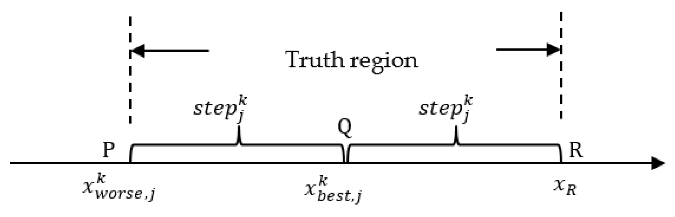
Figure 1 illustrates the principle of the position update. s t e p j k = | x b e s t , j k x w o r s e , j k | is an adaptive step of the jth decision variable in the current iteration k . The range between P and R is referred to as a truth region, which is centered at the global best harmony. In other words, the jth decision variable is generated randomly in a range of the truth region. In the early iteration, all solution vectors in the harmony memory are sporadic, and the truth region is wide, which means that the new harmony is generated randomly in a large range. It is beneficial to enhance the global search ability. In the late iteration, all solution vectors in the HM are inclined to move to the global optimum. Therefore, all solution vectors are concentrated within a small solution space, and the truth region is narrow, which enhances the local search ability of NGHS [13,17,18]. The NGHS algorithm works as follows.
• Step 1: Initialize the algorithm and problem parameters
The genetic mutation probability ( p m ), the current iteration k , and the maximum number of iterations (NI) are set in this step. However, the harmony memory considering rate (HMCR), pitch adjusting rate (PAR), and the bandwidth (BW) are excluded from the NGHS algorithm.
• Step 2: Initialize the harmony memory (HM)
The initial values of the decision variable x i , j k = 0   ( i = 1 , , ,   H M S ) are generated by Equation (1). The harmony memory (HM) is shown in Equation (2).
• Step 3: Improvise a new harmony
A new harmony vector x n e w , j k = ( x n e w , 1 k , x n e w , 2 k , , x n e w , D k ) is improvised by Algorithm 3.
Algorithm 3 The Improvisation of New Harmony in NGHS
1: For j = 1 to D do
2:    x R = 2 × x b e s t , j k x w o r s e , j k
3:   If x R > x j U then
4:      x R = x j U
5:   Else if x R < x j L then
6:      x R = x j L
7:   End
8:    x n e w , j k = x w o r s e , j k + r 1 × ( x R x w o r s e , j k ) %position update
9:   If r 2 p m then
10:      x n e w , j k = x j L + r 3 × ( x j U x j L ) % genetic mutation
11:  End
12: End
Here, x b e s t , j k and x w o r s e , j k are the best harmony and the worse harmony in the harmony memory, when the current iteration is k , respectively. r 1 , r 2 , and r 3 are random numbers in the range of [0,1]:
• Step 4: Update the harmony memory
The new harmony replaces the worse harmony in the HM, even if the worse harmony in the HM has better fitness than the new harmony.
• Step 5: Check the stopping iteration
If the current iteration k is equal to the stopping iteration (the maximum number of iterations is NI), the algorithm is terminated. Otherwise, set k = k + 1 and go back to step 3.

3. Selective Acceptance Novel Global Harmony Search Algorithm

Assad et al. [19] pointed that the effectiveness of evolutionary algorithms relies on the extent of balance between diversification, which implies the ability of an algorithm to explore the high performance regions of the search space, and intensification, which is the ability of an algorithm to search for better solution in the high performance regions during the optimizing process. In other words, the key to improving the searching ability of evolutionary algorithms is to enhance the extent of balance between diversification and intensification capabilities. It can be seen that, in Section 2, Step 3 (Improvise a new harmony) in the IHS, SGHS, or NGHS algorithm is gradually improved to balance the diversification and intensification capabilities. However, in Step 4, the mechanism of updating the HM is different in these algorithms. Accept-the-better-only mechanism is used in the HS, IHS, and the SGHS algorithm. The accept-everything mechanism is used in the NGHS algorithm. This difference inspired us to explore whether the mechanism in Step 4 could affect the balance of diversification and intensification capabilities and improve the searching ability of the NGHS algorithm. However, in the process of finding a good mechanism in Step 4, the mechanism that is used in the SA algorithm attracted our attention. The SA algorithm used Boltzmann distribution to calculate the acceptable probability dynamically in each iteration and determine to accept the new solution or not by the value of acceptable probability. Therefore, in this paper, we proposed the selective acceptance novel global harmony search (SANGHS) algorithm, which combined the selective acceptance mechanism with the NGHS algorithm.
The main difference between the SANGHS and the NGHS algorithms is that the SANGHS algorithm will accept and replace the worst harmony in the HM with the new harmony according to the selective acceptance mechanism. In this mechanism, the selective acceptance formula as shown in Equation (6), which is also dynamically adjusted in the optimization process as in the SA algorithm, is used to further balance the diversification and intensification capabilities. However, the selective acceptance formula is different from the Boltzmann distribution in the SA algorithm and does not need to use additional parameters. In Equation (6), A P k represents the acceptable probability in the current iteration k . F n e w k represents the fitness value of the new harmony in the current iteration k . F b e s t k and F w o r s e k represent the fitness values of the best and the worst harmonies in the HM in the current iteration k , respectively. According to the selective acceptance formula in the SANGHS algorithm, if the fitness of the new harmony is better than the worst harmony in the HM, the AP is equal to 1. It means that the worst harmony will be replaced by the new harmony in the HM. However, if the fitness of the new harmony is worse than the worst harmony in the HM, the SANGHS algorithm will accept the new harmony according to the AP, which is calculated by the proportion formula. Proportion formula is the most important part of the selective acceptance formula. In proportion formula, F w o r s e k F b e s t k represents the convergence degree of all harmonies in the HM. In the early iterations, all harmonies in the HM are dispersed in a large solution space, and the value of F w o r s e k F b e s t k is a large value. Thus, it is more likely to accept a worse harmony and thereby expand the range of truth region in the SANGHS algorithm, which would contribute to improve the diversification capabilities. Conversely, in the late iterations, all harmonies in the HM have converged in a small solution space; the value of F w o r s e k F b e s t k is a small value. The HM is less likely to accept a worse harmony and thereby reduce the range of truth region, which makes the SANGHS algorithm have strong intensification capabilities:
A P k = { 1 i f   F n e w k F w o r s e k ( F w o r s e k F b e s t k ) ( F n e w k F b e s t k ) i f   F n e w k > F w o r s e k
In general, the SANGHS algorithm contains the following steps:
• Step 1: Initialize the algorithm and problem parameters
The genetic mutation probability ( p m ), the current iteration k , and the maximum iteration (NI) are set in this step.
• Step 2: Initialize the harmony memory (HM)
The initial values of the decision variable x i , j k = 0   ( i = 1 , 2 , ,   H M S ) are generated by Equation (1). The harmony memory (HM) is shown in Equation (2).
• Step 3: Improvise a new harmony
A new harmony vector x n e w , j k = ( x n e w , 1 k , x n e w , 2 k , , x n e w , D k ) is improvised by Algorithm 3. This step is the same as in the NGHS algorithm.
• Step 4: Calculate AP
If the new harmony has a better fitness value than the worst harmony in the HM, AP is set to 1. Otherwise, AP is calculated by Equation (6).
• Step 5: Update the harmony memory
Firstly, generate a random number in [0,1]. If the random number is smaller than the AP, the new harmony replaces the worst harmony in the HM. Otherwise, the new harmony is discarded.
• Step 6: Check the stopping iteration
If the current iteration k is equal to the stopping iteration (the maximum number of iterations is NI), the algorithm is terminated. Otherwise, set k = k + 1 and go back to Step 3.

4. Experimental Results and Analysis

4.1. Computing Environment Settings

In this study, we used Python 3.5.1 (64-bit) as the complier to implement the program to search for the trial solution. The solution-finding equipment comprised an Intel Core (TM) i5-8500 (3.0 GHz, 3.0 GHz) CPU, 8 GB of memory, and Windows 10 professional edition (64-bit) OS.

4.2. Ten Well-Known Benchmark Optimization Problems

To estimate the performance for the proposed acceptable probability mechanism, we considered ten well-known benchmark optimization problems [20,21] as follows. Among these problems, problems 1 to 4 are unimodal problems. Problems 5 to 10 are multimodal problems with several local optima, and the number of local optima is increased with the number of decision variables [12].
(1)
Sphere function (F1)
The Sphere function is defined as m i n   f ( x i ) = i = 1 N x i 2 , where the global optimum is 0, and the search space of x i   ( i = 1 , 2 , , N ) is [ 100 ,   100 ] .
(2)
Schwedel’s problem 2.22 (F2)
This problem is defined as m i n   f ( x i ) = i = 1 N | x i | + i = 1 N | x i | , where the global optimum is 0, and the search space of x i   ( i = 1 , 2 , , N ) is [ 10 , 10 ] .
(3)
Axis Parallel Function (F3)
This problem is defined as min f ( x i ) = i = 1 N i x i 2 , where the global optimum is 0, and the search space of x i   ( i = 1 , 2 , , N ) is [ 5.12 , 5.12 ] .
(4)
Quartic Function (F4)
This problem is defined as min f ( x i ) = i = 1 N x i 4 , where the global optimum is 0, and the search space of x i   ( i = 1 , 2 , , N ) is [ 1.28 , 1.28 ] .
(5)
Ackley’s function (F5)
The Ackley’s function is defined as m i n   f ( x i ) = 20 + e 20 e x p ( 0.2 i = 1 N x i 2 N ) e x p ( i = 1 N c o s ( 2 π x i ) N ) , where the global optimum is 0, and the search space of x i   ( i = 1 , 2 , , N ) is [ 32 , 32 ] .
(6)
Rastrigin function (F6)
The Rastrigin function is defined as m i n   f ( x i ) = i = 1 N ( x i 2 10 c o s ( 2 π x i ) + 10 ) , where the global optimum is 0, and the search space of x i   ( i = 1 , 2 , , N ) is [ 5.12 , 5.12 ] .
(7)
Schwefel’s problem 2.26 (F7)
This problem is defined as m i n   f ( x i ) = 418.9829 N i = 1 N ( x i s i n ( | x i | ) ) , where the global optimum is 0, and the search space of x i   ( i = 1 , 2 , , N ) is [ 500 , 500 ] .
(8)
Levy Function (F8)
This problem is defined as m i n   f ( x i ) = sin 2 ( π w 1 ) i = 1 N 1 ( w i 1 ) 2 [ 1 + 10 s i n 2 ( π w i + 1 ) ] + ( w N 1 ) 2 [ 1 + s i n 2 ( 2 π w D ) ] , where w i = 1 + x i 1 4 and the global optimum is 0, and the search space of x i   ( i = 1 , 2 , , N ) is [ 10 , 10 ] .
(9)
Bohachevsky function (F9)
This problem is defined as m i n   f ( x i ) = i = 1 N 1 [ x i 2 + 2 x i + 1 2 0.3 cos ( 3 π x i ) 0.4 cos ( 4 π x i + 1 ) + 0.7 ] , where the global optimum is 0, and the search space of x i   ( i = 1 , 2 , , N ) is [ 15 , 15 ] .
(10)
Alpine 1 function (F10)
This problem is defined as m i n   f ( x i ) = i = 1 N | x i sin ( x i ) + 0.1 x i | , where the global optimum is 0, and the search space of x i   ( i = 1 , 2 , , N ) is [ 10 , 10 ] .

4.3. Comparison of Different Harmony Search Algorithms in Ten Benchmark Optimization Problems

To test the performance of the SANGHS algorithm for ten aforementioned optimization problems, we compared it with four harmony search algorithms, which were the HS, IHS, SGHS, and NGHS algorithms. The parameters of these algorithms are provided in Table 1 [12,17,22,23]. We tested three different dimensions equal to 10, 30, and 100. The maximum number of iterations (NI) is set to 30,000 with D = 10, 60,000 with D = 30, and 150,000 with D = 100. Each problem was tested in 30 independent experiments. The experimental results for all problems with three different dimensions obtained by the four harmony search algorithms and the SANGHS algorithm are shown in Table 2, Table 3 and Table 4. Mean and Std represent the average and the standard deviation of 30 independent experiments, respectively, as provided in Table 2, Table 3 and Table 4. Min and Max represent the minimum and maximum fitness values in 30 independent experiments.
In Table 2, Table 3 and Table 4, several experimental results are given. Firstly, in all problems (F1 to F10) with three different dimensions (D = 10, 30, and 100), the SANGHS algorithm has smaller minimum (Min) and maximum (Max) fitness values than other four HS algorithms. For example, in problem 1 with D = 10, SANGHS has the smallest minimum fitness values (9.6086 × 10−111) and the smallest maximum fitness values (1.3918 × 10−77). Secondly, the SANGHS algorithm has a smallest average (Mean) fitness value. For example, in problem 1 with D = 10, SANGHS has the smallest average fitness values (4.6889 × 10−79). This value is far less than the second one (8.2477 × 10−38). The above two experimental results reveal that the SANGHS algorithm has a better search ability than other four harmony search algorithms. Lastly, in the above problems (F1 to F10) with D = 10, 30, and 100, the SANGHS algorithm has a smallest standard deviation (Std) value. For example, in problem 1 with D = 10, SANGHS has the smallest standard deviation values (2.4976 × 10−78), and this value is also far less than the second one (3.8833 × 10−37). It means that the search ability of the SANGHS algorithm is more robust than other four harmony search algorithms.
In addition, to further explore the difference in the performance of the SANGHS algorithm and other four harmony search algorithms, the experiment results were also analyzed through the Wilcoxon rank-sum test [24,25] as shown in Table 5. In Table 5, the p-value, which is greater than 0.05, is bold. Based on the p-value, the SANGHS algorithm is significantly better than the other four HS algorithms in all problems with three different dimensions, except in problem 10 (F10) with D = 10 (6.3886 × 10⁻²).
Figure 2 shows the typical convergence graphs of five different algorithms for ten problems with D = 30. In Figure 2a–d which are unimodal problems, as the number of iterations increases, the SANGHS algorithm converges faster than other four harmony search algorithms. It means that the SANGHS algorithm has a strong local search ability in unimodal problems. In Figure 2e,f,h,j which are multimodal problems, we can easily observe that the SANGHS algorithm is more effective in escaping from the local optima and have a better convergence ability compared with the other four harmony search algorithms. In other words, the SANGHS algorithm has a better balance between the global search ability and the local search ability in multimodal problems.

4.4. Two Benchmarks’ Engineering Optimization Problems

In this section, to verify the searching performance of the SANGHS algorithm further, we used the SANGHS algorithm to solve two benchmark engineering problems and compared the experimental results with previous references [26,27,28,29,30,31,32,33,34,35,36,37,38].

4.4.1. Tension/Compression Spring Design Optimization Problem

The first engineering problem is the tension/compression spring design engineering problem. The main purpose of this problem is to minimize the spring weight by determining three design variables when four constraints are satisfied. Three design variables are the wire diameter (d), mean coil diameter (D), and the number of active coils (N). Four constraints are about the shear stress, surge frequency, and the minimum deflection. One objective function, three design variables, and four constraints are shown in Figure 3.
We used the HS, IHS, SGHS, NGHS, and the SANGHS algorithms to search the best result for this problem. Table 6 shows the parameters of these five HS algorithms. The best results obtained by these five algorithms are shown in Table 7. Moreover, as shown in Table 7, to further verify the searching performance of SANGHS algorithm, the best result of SANGHS algorithm is also compared with other state-of-the-art algorithms which have been applied to solve this problem.
In Table 7, it can be seen that, compared with the HS, IHS, SGHS, and the NGHS algorithm, the SANGHS algorithm provides a best fitness value for the tension/compression spring design engineering problem. It is worth noting that the SANGHS algorithm also provides a very competitive result compared with the other state-of-the-art algorithms in previous works.

4.4.2. Welded Beam Design Optimization Problem

The second problem is the welded beam design engineering problem. In this problem, there are four variables that need to be determined that are the thickness of the weld ( x 1 ), the length of the clamped bar ( x 2 ), the height of the bar ( x 3 ), and the thickness of the bar ( x 4 ). The main purpose of this problem is to minimize the manufacturing cost when seven constraints are satisfied. The constraints include limits on the shear stress, bending stress, buckling load and end deflection, and several size constraints. The welded beam and its design variables are shown in Figure 4. These seven constraints and the objective function of manufacturing cost are defined as follows.
We also used the HS, IHS, SGHS, NGHS, and the SANGHS algorithms to search the best result for this problem. Table 8 shows the parameters of these five HS algorithms. The best results obtained by these five algorithms are shown in Table 9. Moreover, as shown in Table 9, to further verify the searching performance of SANGHS algorithm, the best result of the SANGHS algorithm is also compared with other state-of-the-art algorithms that have been applied to solve this problem.
In Table 9, it can be seen that, compared with the HS, IHS, SGHS, and the NGHS algorithm, the SANGHS algorithm provides a minimum manufacturing cost for the welded beam design engineering problem. It is worth noting that the SANGHS algorithm also provides a very competitive result compared with other state-of-the-art algorithms in previous works.

5. Conclusions

In this paper, we presented a novel algorithm, called the SANGHS algorithm, which combines the NGHS algorithm with a selective acceptance mechanism. In the SANGHS algorithm, the acceptable probability (AP) is generated by a selective acceptance formula in each iteration. Based on the value of AP, the SANGHS algorithm will determine whether to accept the worse trial solution or not. Moreover, to verify the searching performance of the SANGHS algorithm, we used the SANGHS algorithm in ten well-known benchmark continuous optimization problems and two engineering problems and compared the experimental results with other state-of-the-art metaheuristic algorithms. The experimental results provide two findings that are worth noting.
Firstly, it was found that the SANGHS algorithm could result in improved searching performance as opposed to the NGHS algorithm. In the SANGHS algorithm, the selective acceptance mechanism dynamically adjusts the acceptable probability according to the selective acceptance formula. The most important part of the selective acceptance formula is proportion formula, and the main concept of the proportion formula is convergence degree in the HM. Hence, in Equation (6), F w o r s e k F b e s t k represents the convergence degree of all harmonies in the HM. In the early iterations, all solutions have not yet converged in the HM. Therefore, the value of F w o r s e k F b e s t k will be a larger value, and then there is a larger acceptable probability to accept a worse harmony. In the next iteration, there is a higher probability to generate a new harmony in a larger truth region. In other words, there is a strong global exploration ability in the early iterations. However, in the late iterations, the value of F w o r s e k F b e s t k will be a smaller value while all solutions have converged in the HM. Therefore, there is a smaller acceptable probability to accept a worse harmony. In the next iteration, there is a higher probability to generate a new harmony in a smaller truth region. In other words, there is a strong local exploitation ability in the later iterations. According to the experimental results, the proposed proportion mechanism can balance the global exploration and local exploitation ability in the NGHS algorithm.
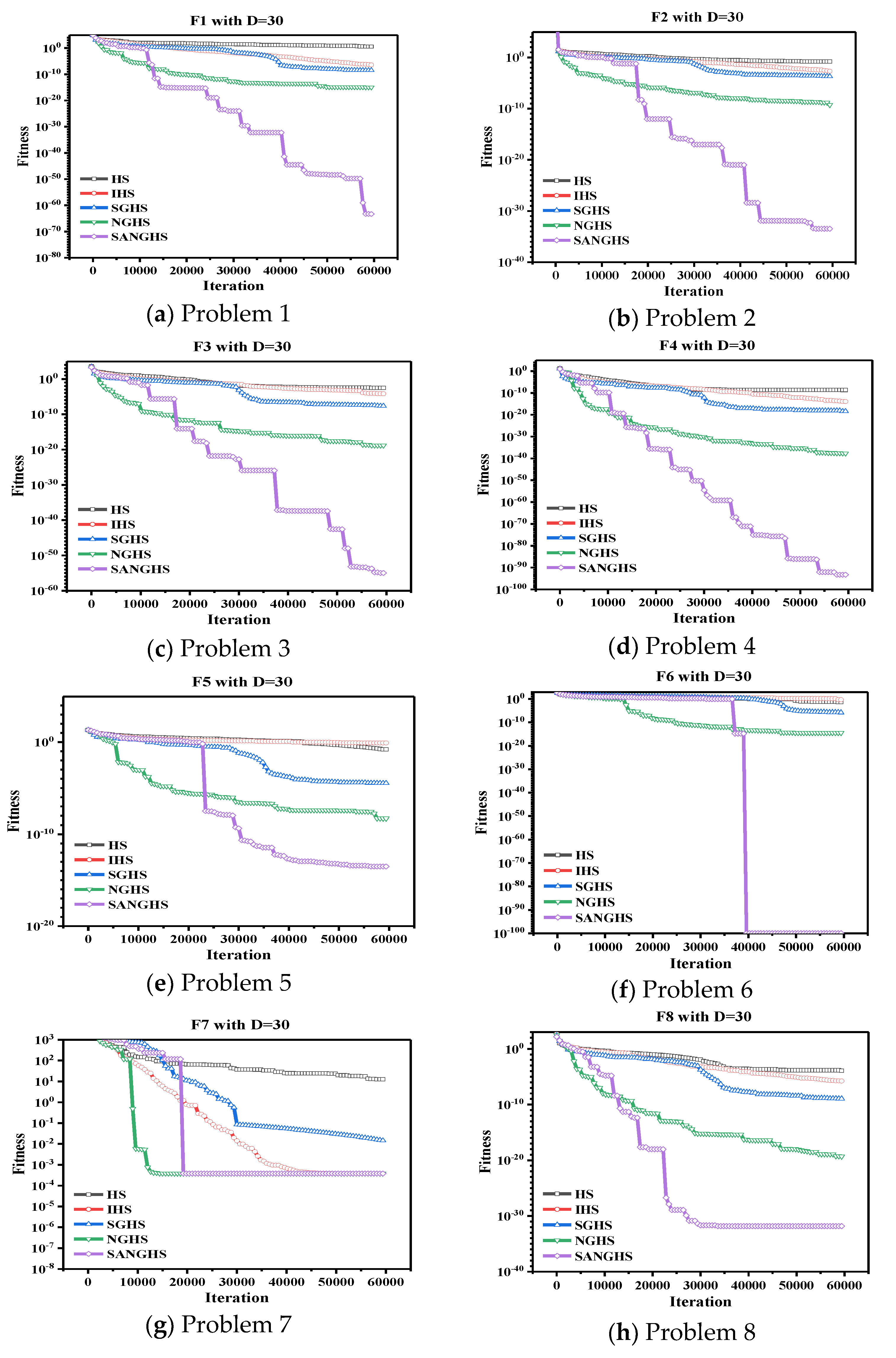
Finally, in ten considered benchmark optimization problems with three different dimensions, based on the results of the Wilcoxon rank-sum test and the convergence graphs, the searching performance of the SANGHS algorithm was better than other four HS algorithms significantly. Especially in Figure 2, we can easily observe that the SANGHS algorithm had the better searching performance and convergence ability than other algorithms in all problems. Conversely, the HS, IHS, and the SGHS algorithms easily fall within the local optimum, and unlikely escape it. Moreover, in two engineering optimization problems, the SANGHS algorithm could not only search for a better solution compared with other four HS algorithms, but also could provide a competition result to compare with other state-of-the-art algorithms. In conclusion, the SANGHS algorithm is a more efficient and effective algorithm.

Author Contributions

Conceptualization, P.-C.S. and H.L.; Formal analysis, H.L. and L.H.; Methodology, H.L.; Software, H.L.; Supervision, X.Z. and C.Y.; Validation, H.L. and P.-C.S.; Writing—original draft, H.L.; Writing—review and editing, P.-C.S. and H.L. All authors have read and agreed to the published version of the manuscript.

Funding

This research was funded by the National Natural Science Foundation of China, Grant No. 71840003.

Acknowledgments

The authors would like to thank all the reviewers for their constructive comments.

Conflicts of Interest

The authors declare no conflict of interest.

References

  1. Lee, K.S.; Geem, Z.W.; Lee, S.H.; Bae, K.W. The harmony search heuristic algorithm for discrete structural optimization. Eng. Optim. 2005, 37, 663–684. [Google Scholar] [CrossRef]
  2. Geem, Z.W. Optimal cost design of water distribution networks using harmony search. Eng. Optim. 2006, 38, 259–280. [Google Scholar] [CrossRef]
  3. Geem, Z.W.; Lee, K.S.; Park, Y. Application of Harmony Search to Vehicle Routing. Am. J. Appl. Sci. 2005, 12, 1552–1557. [Google Scholar] [CrossRef] [Green Version]
  4. Metawaa, N.; Hassana, M.K.; Elhoseny, M. Genetic algorithm based model for optimizing bank lending decisions. Expert Syst. Appl. 2017, 80, 75–82. [Google Scholar] [CrossRef]
  5. Chen, K.H.; Chen, L.F.; Su, C.T. A new particle swarm feature selection method for classification. J. Intell. Inf. Syst. 2014, 42, 507–530. [Google Scholar] [CrossRef]
  6. Lee, K.S.; Geem, Z.W. A new meta-heuristic algorithm for continuous engineering optimization: Harmony search theory and practice. Comput. Methods Appl. Mech. Eng. 2005, 194, 3902–3933. [Google Scholar] [CrossRef]
  7. Afshar, A.; Bozorg Haddad, O.; Mariño, M.A.; Adams, B.J. Honey-bee mating optimization (HBMO) algorithm for optimal reservoir operation. J. Franklin Inst. 2007, 344, 452–462. [Google Scholar] [CrossRef]
  8. Sanchis, J.; Martínez, M.A.; Blasco, X. Integrated multiobjective optimization and a priori preferences using genetic algorithms. Inf. Sci. 2008, 178, 931–951. [Google Scholar] [CrossRef]
  9. Zhang, J.; Zhang, Y.; Gao, R. Genetic algorithms for optimal design of vehicle suspensions. In Proceedings of the IEEE International Conference on Engineering of Intelligent Systems, Islamabad, Pakistan, 22–23 April 2006. [Google Scholar]
  10. Marinakis, Y.; Marinaki, M.; Dounias, G. Particle swarm optimization for pap-smear diagnosis. Expert Syst. Appl. 2008, 35, 1645–1656. [Google Scholar] [CrossRef]
  11. Mahdavi, M.; Fesanghary, M.; Damangir, E. An improved harmony search algorithm for solving optimization problems. Appl. Math. Comput. 2007, 188, 1567–1579. [Google Scholar] [CrossRef]
  12. Pan, Q.K.; Suganthan, P.N.; Tasgetiren, M.F.; Liang, J.J. A self-adaptive global best harmony search algorithm for continuous optimization problems. Appl. Math. Comput. 2010, 216, 830–848. [Google Scholar] [CrossRef]
  13. Zou, D.; Gao, L.; Li, S.; Wu, J.; Wang, X. A novel global harmony search algorithm for task assignment problem. J. Syst. Softw. 2010, 83, 1678–1688. [Google Scholar] [CrossRef]
  14. Nowicki, E.; Smutnicki, C. A fast tabu search algorithm for the permutation flow-shop problem. Eur. J. Oper. Res. 1996, 91, 160–175. [Google Scholar] [CrossRef]
  15. Metropolis, N.; Rosenbluth, A.W.; Rosenbluth, M.N.; Teller, A.H.; Teller, E. Equation of state calculations by fast computing machines. J. Chem. Phys. 1953, 21, 1087–1092. [Google Scholar] [CrossRef] [Green Version]
  16. Chiu, C.Y.; Shih, P.C.; Li, X. A dynamic adjusting novel global harmony search for continuous optimization problems. Symmetry 2018, 10, 337. [Google Scholar] [CrossRef] [Green Version]
  17. Zou, D.; Gao, L.; Wu, J.; Li, S. Novel global harmony search algorithm for unconstrained problems. Neurocomputing 2010, 73, 3308–3318. [Google Scholar] [CrossRef]
  18. Zou, D.; Gao, L.; Wu, J.; Li, S.; Li, Y. A novel global harmony search algorithm for reliability problems. Comput. Ind. Eng. 2010, 58, 307–316. [Google Scholar] [CrossRef]
  19. Assad, A.; Deep, K. A two-phase harmony search algorithm for continuous optimization. Comput. Intell. 2017, 33, 1038–1075. [Google Scholar] [CrossRef]
  20. Jamil, M.; Yang, X.S. A literature survey of benchmark functions for global optimisation problems. Int. J. Math. Model. Numer. Optim. 2013, 4, 150–194. [Google Scholar] [CrossRef] [Green Version]
  21. Laguna, M.; Martí, R. Experimental testing of advanced scatter search designs for global optimization of multimodal functions. J. Glob. Optim. 2005, 33, 235–255. [Google Scholar] [CrossRef]
  22. Tavakoli, S.; Valian, E.; Mohanna, S. Feedforward neural network training using intelligent global harmony search. Evol. Syst. 2012, 3, 125–131. [Google Scholar] [CrossRef]
  23. Valian, E.; Tavakoli, S.; Mohanna, S. An intelligent global harmony search approach to continuous optimization problems. Appl. Math. Comput. 2014, 232, 670–684. [Google Scholar] [CrossRef]
  24. Wilcoxon, F. Individual Comparisons by Ranking Methods. Biom. Bull. 1945, 1, 80–83. [Google Scholar] [CrossRef]
  25. García, S.; Molina, D.; Lozano, M.; Herrera, F. A study on the use of non-parametric tests for analyzing the evolutionary algorithms’ behaviour: A case study on the CEC’2005 Special Session on Real Parameter Optimization. J. Heuristics 2009, 12, 15–617. [Google Scholar] [CrossRef]
  26. Heidari, A.A.; Mirjalili, S.; Faris, H.; Aljarah, I.; Mafarja, M.; Chen, H. Harris hawks optimization: Algorithm and applications. Futur. Gener. Comput. Syst. 2019, 97, 849–872. [Google Scholar] [CrossRef]
  27. Mirjalili, S.; Mirjalili, S.M.; Lewis, A. Grey Wolf Optimizer. Adv. Eng. Softw. 2014, 69, 46–61. [Google Scholar] [CrossRef] [Green Version]
  28. Kaveh, A.; Khayatazad, M. A new meta-heuristic method: Ray Optimization. Comput. Struct. 2012, 112–113, 283–294. [Google Scholar] [CrossRef]
  29. Huang, F.; Wang, L.; He, Q. An effective co-evolutionary differential evolution for constrained optimization. Appl. Math. Comput. 2007, 186, 340–356. [Google Scholar] [CrossRef]
  30. He, Q.; Wang, L. An effective co-evolutionary particle swarm optimization for constrained engineering design problems. Eng. Appl. Artif. Intell. 2007, 20, 89–99. [Google Scholar] [CrossRef]
  31. Coello, C.A.C.; Montes, E.M. Constraint-handling in genetic algorithms through the use of dominance-based tournament selection. Adv. Eng. Inform. 2002, 16, 193–203. [Google Scholar] [CrossRef]
  32. Mezura-Montes, E.; Coello, C.A.C. An empirical study about the usefulness of evolution strategies to solve constrained optimization problems. Int. J. Gen. Syst. 2008, 37, 443–473. [Google Scholar] [CrossRef]
  33. Mirjalili, S.; Lewis, A. The Whale Optimization Algorithm. Adv. Eng. Softw. 2016, 95, 51–67. [Google Scholar] [CrossRef]
  34. Mirjalili, S. Moth-flame optimization algorithm: A novel nature-inspired heuristic paradigm. Knowl. -Based Syst. 2015, 89, 228–249. [Google Scholar] [CrossRef]
  35. Heidari, A.A.; Abbaspour, A.R.; Jordehi, A.R. An efficient chaotic water cycle algorithm for optimization tasks. Neural Comput. Appl. 2017, 28, 57–85. [Google Scholar] [CrossRef]
  36. Li, Y.; Li, X.; Liu, J.; Ruan, X. An Improved Bat Algorithm Based on Lévy Flights and Adjustment Factors. Symmetry 2019, 7, 925. [Google Scholar] [CrossRef] [Green Version]
  37. Deb, K. Optimal design of a welded beam via genetic algorithms. AIAA J. 1991, 29, 2013–2015. [Google Scholar] [CrossRef]
  38. Ragsdell, K.M.; Phillips, D.T. Optimal Design of a Class of Welded Structures Using Geometric Programming. Am. Soc. Mech. Eng. 1975, 1021–1025. [Google Scholar] [CrossRef]
Figure 1. Schematic diagram of position update.
Applsci 10 01910 g001
Figure 2. Typical convergence graph of five different algorithms for ten problems with D = 30. (a) problem 1; (b) problem 2; (c) problem 3; (d) problem 4; (e) problem 5; (f) problem 6; (g) problem 7; (h) problem 8; (i) problem 9; (j) problem 10.
Applsci 10 01910 g002aApplsci 10 01910 g002b
Figure 3. Tension/compression spring design.
Applsci 10 01910 g003
Figure 4. Welded beam design.
Applsci 10 01910 g004
Table 1. Parameters of compared harmony search (HS) algorithms in ten optimization problems.
AlgorithmHSIHSSGHSNGHSSANGHS
HMS 155555
HMCR 20.90.9 H M C R m e a n = 0.98
PAR 30.3 P A R m i n = 0.01
P A R m a x = 0.99
P A R m e a n = 0.9
BW 4 B W m i n = 0.0001
B W m a x = ( x j U x j L ) / 20
B W m i n = 0.0005
B W m a x = ( x j U x j L ) / 10
LP 5100
P m 60.0050.005
1 HMS: the harmony memory size; 2 HMCR: the harmony memory considering rate; 3 PAR: the pitch adjusting rate; 4 BW: the bandwidth; 5 LP: the learning period; 6 P m : the genetic mutation probability.
Table 2. Experimental results of five algorithms for 10 problems with D = 10.
No.AlgorithmMinMaxMeanStdNo.AlgorithmMinMaxMeanStd
F1HS5.2096 × 10−81.1157 × 10−62.3562 × 10−71.8902 × 10⁻⁷F6HS8.3112 × 10−67.8214 × 10−53.3076 × 10−51.7982 × 10⁻⁵
IHS6.7803 × 10−92.3518 × 10−81.3575 × 10−83.7943 × 10⁻⁹IHS1.1191 × 10−64.0212 × 10−62.6004 × 10−66.4709 × 10⁻⁷
SGHS6.8178 × 10−121.4106 × 10−103.2650 × 10−112.5506 × 10⁻¹¹SGHS1.1716 × 10−93.8150 × 10−11.2717 × 10−26.8481 × 10⁻²
NGHS1.0698 × 10−452.1604 × 10−368.2477 × 10−383.8833 × 10−37NGHS0.0000 × 1000.0000 × 1000.0000 × 1000.0000 × 100
SANGHS9.6086 × 10−1111.3918 × 10−774.6889 × 10−792.4976 × 10−78SANGHS0.0000 × 1000.0000 × 1000.0000 × 1000.0000 × 100
F2HS3.2109 × 10−41.5971 × 10−37.7726 × 10−42.7372 × 10⁻⁴F7HS1.2731 × 10−42.8515 × 10−21.0739 × 10−35.0957 × 10⁻³
IHS2.0318 × 10−43.6754 × 10−42.9700 × 10−43.2031 × 10⁻⁵IHS1.2728 × 10−41.2728 × 10−41.2728 × 10−44.0700 × 10⁻¹⁰
SGHS7.3565 × 10−61.8055 × 10−51.2027 × 10−52.7866 × 10⁻⁶SGHS1.2728 × 10−42.9759 × 10−41.3517 × 10−43.1705 × 10⁻⁵
NGHS3.8140 × 10−275.1898 × 10−212.3612 × 10−229.4731 × 10⁻²²NGHS1.2728 × 10−41.2728 × 10−41.2728 × 10−48.5769 × 10⁻¹⁴
SANGHS1.4267 × 10−827.2433 × 10−543.5052 × 10−551.4044 × 10−54SANGHS1.2728 × 10−41.2728 × 10−41.2728 × 10−44.4839 × 10⁻¹⁴
F3HS1.4468 × 10−72.1934 × 10−68.0446 × 10−74.2722 × 10⁻⁷F8HS2.0732 × 10−83.4077 × 10−78.0031 × 10−86.4199 × 10⁻⁸
IHS3.1842 × 10−89.8796 × 10−86.2079 × 10−81.8245 × 10⁻⁸IHS3.3581 × 10−91.0209 × 10−86.7715 × 10−91.7956 × 10⁻⁹
SGHS2.7923 × 10−117.2398 × 10−101.7525 × 10−101.4531 × 10⁻¹⁰SGHS1.7990 × 10−125.0988 × 10−111.3622 × 10−111.1253 × 10⁻¹¹
NGHS4.4709 × 10−463.5344 × 10−392.3102 × 10−407.0896 × 10−40NGHS1.4998 × 10−321.4998 × 10−321.4998 × 10−325.4738 × 10−48
SANGHS3.8636 × 10−1134.3798 × 10−832.3947 × 10−849.1559 × 10−84SANGHS1.4998 × 10−321.4998 × 10−321.4998 × 10−325.4738 × 10−48
F4HS2.2666 × 10−173.0752 × 10−147.0687 × 10−158.2181 × 10⁻¹⁵F9HS1.1130 × 10−62.8915 × 10−57.0153 × 10−65.3517 × 10⁻⁶
IHS9.5725 × 10−186.5490 × 10−172.9787 × 10−171.3161 × 10⁻¹⁷IHS3.0585 × 10−79.1446 × 10−75.8587 × 10−71.4754 × 10⁻⁷
SGHS2.5924 × 10−234.7975 × 10−216.9747 × 10−221.1480 × 10⁻²¹SGHS3.2077 × 10−104.1452 × 10−91.3097 × 10−98.5282 × 10⁻¹⁰
NGHS1.9010 × 10−867.5124 × 10−672.5042 × 10−681.3485 × 10−67NGHS5.7250 × 10−492.0380 × 10−367.8672 × 10−383.6838 × 10−37
SANGHS1.7493 × 10−1699.2806 × 10−1243.2904 × 10−1251.6640 × 10−124SANGHS2.0444 × 10−1131.4776 × 10−694.9253 × 10−712.6524 × 10−70
F5HS1.7118 × 10−48.0222 × 10−44.6344 × 10−41.5000 × 10⁻⁴F10HS1.1494 × 10−41.8959 × 10−34.9240 × 10−43.4263 × 10⁻⁴
IHS1.0584 × 10−41.6838 × 10−41.4686 × 10−41.5429 × 10⁻⁵IHS2.0995 × 10−53.2351 × 10−45.9924 × 10−57.1295 × 10⁻⁵
SGHS2.8256 × 10−61.2840 × 10−56.6281 × 10−62.4208 × 10⁻⁶SGHS5.6467 × 10−71.8978 × 10−55.9487 × 10−65.4367 × 10⁻⁶
NGHS6.6613 × 10−153.8636 × 10−141.8267 × 10−147.1015 × 10⁻¹⁵NGHS1.4433 × 10−151.5821 × 10−146.1063 × 10−153.0077 × 10⁻¹⁵
SANGHS6.6613 × 10−152.7978 × 10−141.4122 × 10−144.8842 × 10⁻¹⁵SANGHS8.3267 × 10−161.0658 × 10−144.9442 × 10−152.5741 × 10⁻¹⁵
Table 3. Experimental results of five algorithms for 10 problems with D = 30.
No.AlgorithmMinMaxMeanStdNo.AlgorithmMinMaxMeanStd
F1HS5.0536 × 10−16.4171 × 1003.3124 × 1001.5861 × 100F6HS2.6666 × 10−22.0462 × 1005.0288 × 10−16.0096 × 10⁻¹
IHS2.1207 × 10−74.9163 × 10−73.5819 × 10−77.1968 × 10⁻⁸IHS4.0261 × 10−54.6986 × 1001.3178 × 1001.0352 × 100
SGHS1.5978 × 10−91.4781 × 10−84.8841 × 10−93.1202 × 10⁻⁹SGHS7.9528 × 10−79.9496 × 10−14.8052 × 10−21.8483 × 10⁻¹
NGHS1.2081 × 10−176.1930 × 10−156.6153 × 10−161.3269 × 10⁻¹⁵NGHS0.0000 × 1004.7713 × 10−121.7243 × 10−138.5424 × 10⁻¹³
SANGHS2.3793 × 10−662.4404 × 10−378.1347 × 10−394.3807 × 10−38SANGHS0.0000 × 1000.0000 × 1000.0000 × 1000.0000 × 100
F2HS4.5085 × 10−22.0043 × 10−17.6210 × 10−23.7203 × 10⁻²F7HS8.1324 × 1005.2395 × 1012.0713 × 1019.5235 × 100
IHS1.7655 × 10−34.4854 × 10−32.3905 × 10−34.6485 × 10⁻⁴IHS3.8186 × 10−41.7516 × 1006.3827 × 10−23.1460 × 10⁻¹
SGHS8.1564 × 10−51.9686 × 10−41.5091 × 10−42.9858 × 10⁻⁵SGHS3.8277 × 10−47.8715 × 10−21.7508 × 10−21.9421 × 10⁻²
NGHS3.2148 × 10−108.7017 × 10−92.0345 × 10−91.7972 × 10⁻⁹NGHS3.8183 × 10−43.8183 × 10−43.8183 × 10−48.1680 × 10⁻¹²
SANGHS1.3727 × 10−447.3787 × 10−282.4752 × 10−291.3243 × 10⁻²⁸SANGHS3.8183 × 10−43.8183 × 10−43.8183 × 10−41.0918 × 10⁻¹³
F3HS1.5858 × 10−34.8414 × 10−32.9867 × 10−37.1956 × 10⁻⁴F8HS5.1397 × 10−51.6213 × 10−41.0240 × 10−42.2064 × 10⁻⁵
IHS8.1295 × 10−61.3227 × 10−31.7068 × 10−43.1223 × 10⁻⁴IHS1.1278 × 10−74.7712 × 10−68.2210 × 10−71.0175 × 10⁻⁶
SGHS8.4500 × 10−95.2306 × 10−82.1700 × 10−81.1042 × 10⁻⁸SGHS3.0351 × 10−101.4228 × 10−97.3604 × 10−102.3859 × 10⁻¹⁰
NGHS3.4329 × 10−193.4291 × 10−161.8533 × 10−176.0640 × 10⁻¹⁷NGHS9.6185 × 10−207.8833 × 10−178.7557 × 10−181.8706 × 10⁻¹⁷
SANGHS9.6420 × 10−702.0955 × 10−487.4888 × 10−503.7563 × 10−49SANGHS1.4998 × 10−321.4998 × 10−321.4998 × 10−325.4738 × 10−48
F4HS9.2705 × 10−104.8468 × 10−93.1521 × 10−99.6498 × 10⁻¹⁰F9HS7.5871× 10−33.2014× 1001.0965× 1001.0189× 100
IHS2.3766 × 10−152.5488 × 10−148.1771 × 10−154.4175 × 10⁻¹⁵IHS8.6839× 10−62.1440× 1005.3391× 10−15.8893× 10⁻¹
SGHS1.9509 × 10−201.6666 × 10−184.2398 × 10−194.2829 × 10⁻¹⁹SGHS3.1568× 10−81.2410× 10−77.9116× 10−82.4154× 10⁻⁸
NGHS1.8030 × 10−406.0162 × 10−354.2247 × 10−361.1809 × 10⁻³⁵NGHS4.2058× 10−191.3275× 10−141.0821× 10−152.8017× 10⁻¹⁵
SANGHS2.6142 × 10−943.9928 × 10−691.3328 × 10−707.1669 × 10−70SANGHS6.1353 × 10−656.3460 × 10−332.3282 × 10−341.1387 × 10⁻³³
F5HS1.5649 × 10−21.7072 × 1006.7498 × 10−13.9769 × 10⁻¹F10HS2.4004 × 10−21.9367 × 10−11.0981 × 10−14.6542 × 10⁻²
IHS3.2084 × 10−41.3089 × 1003.6401 × 10−14.4719 × 10⁻¹IHS2.1852 × 10−29.7546 × 10−25.3262 × 10−21.9894 × 10⁻²
SGHS2.5647 × 10−54.6874 × 10−53.2244 × 10−55.0051 × 10⁻⁶SGHS1.2359 × 10−51.4067 × 10−31.0235 × 10−42.4394 × 10⁻⁴
NGHS7.4210 × 10−101.4597 × 10−84.6791 × 10−93.5652 × 10⁻⁹NGHS1.0805 × 10−103.0740 × 10−98.6347 × 10−106.8488 × 10⁻¹⁰
SANGHS3.8636 × 10−142.9798 × 10−136.2321 × 10−144.5175 × 10⁻¹⁴SANGHS4.4409 × 10−152.1261 × 10−141.1208 × 10−144.4960 × 10⁻¹⁵
Table 4. Experimental results of five algorithms for 10 problems with D = 100.
No.AlgorithmMinMaxMeanStdNo.AlgorithmMinMaxMeanStd
F1HS8.7644 × 1031.6480 × 1041.2203 × 1041.5403 × 103F6HS2.2313 × 1022.9442 × 1022.5974 × 1022.1788 × 101
IHS9.1067 × 1031.4800 × 1041.2428 × 1041.0779 × 103IHS1.9487 × 1022.8076 × 1022.4522 × 1022.0779 × 101
SGHS8.7681 × 10−12.6029 × 1001.3666 × 1004.2374 × 10−1SGHS1.5762 × 1008.5459 × 1004.0935 × 1001.5444 × 100
NGHS4.8032 × 10−41.0576 × 10−37.3694 × 10−41.6006 × 10⁻⁴NGHS1.5643 × 10−32.0192 × 1004.7179 × 10−16.1547 × 10⁻¹
SANGHS5.1238 × 10−237.0729 × 10−154.3965 × 10−161.3365 × 10⁻¹⁵SANGHS0.0000 × 1001.3856 × 10−136.5133 × 10−152.4832 × 10⁻¹⁴
F2HS5.0156 × 1017.3451 × 1016.1118 × 1014.9536 × 100F7HS4.5600 × 1037.0794 × 1035.8498 × 1035.8361 × 102
IHS5.1843 × 1016.8563 × 1016.0248 × 1014.3861 × 100IHS4.4499 × 1036.5893 × 1035.5203 × 1034.9043 × 102
SGHS8.1631 × 10−24.1138 × 10−12.4863 × 10−18.1339 × 10⁻²SGHS8.9612 × 1003.0848 × 1011.7210 × 1015.3463 × 100
NGHS9.9950 × 10−31.6514 × 10−21.3619 × 10−21.5409 × 10⁻³NGHS3.9466 × 10−31.1539 × 10−11.6436 × 10−22.4948 × 10⁻²
SANGHS2.2360 × 10−122.2218 × 10−31.9072 × 10−45.5550 × 10⁻⁴SANGHS1.2728 × 10−31.2728 × 10−31.2728 × 10−34.8314 × 10⁻¹²
F3HS9.4087 × 1021.5941 × 1031.1913 × 1031.6577 × 102F8HS2.4107 × 1013.3570 × 1012.9300 × 1012.8794 × 100
IHS9.2595 × 1021.5737 × 1031.1718 × 1031.4788 × 102IHS2.3183 × 1013.6516 × 1012.9135 × 1013.1786 × 101
SGHS6.4869 × 10−55.3603 × 10−38.8126 × 10−41.2161 × 10⁻³SGHS4.4458 × 10−74.0334 × 10−42.2728 × 10−58.2115 × 10⁻⁵
NGHS3.3424 × 10−51.1541 × 10−46.4369 × 10−51.9242 × 10⁻⁵NGHS1.4748 × 10−69.2715 × 10−63.6238 × 10−61.4865 × 10⁻⁶
SANGHS7.2707 × 10−221.4056 × 10−137.1676 × 10−152.6377 × 10⁻¹⁴SANGHS4.8189 × 10−319.5129 × 10−173.2482 × 10−181.7065 × 10⁻¹⁷
F4HS1.3307 × 10−12.6181 × 10−11.9974 × 10−13.4152 × 10⁻²F9HS7.0005 × 1021.1205 × 1039.0061 × 1021.0327 × 102
IHS1.3301 × 10−12.8520 × 10−12.0499 × 10−13.3111 × 10⁻²IHS7.3029 × 1021.1882 × 1039.1884 × 1021.0628 × 102
SGHS4.0943 × 10−151.1631 × 10−147.5656 × 10−152.0292 × 10⁻¹⁵SGHS2.5895 × 10−14.6678 × 1002.0793 × 1001.0991 × 100
NGHS8.7725 × 10−167.2065 × 10−152.3953 × 10−151.7313 × 10⁻¹⁵NGHS3.4107 × 10−41.4657 × 10−37.7456 × 10−42.5196 × 10⁻⁴
SANGHS6.1762 × 10−464.0280 × 10−311.4178 × 10−327.2252 × 10⁻³²SANGHS2.8823 × 10−221.6936 × 10−151.6201 × 10−163.2735 × 10⁻¹⁶
F5HS1.0843 × 1011.2640 × 1011.1775 × 1014.3937 × 10−1F10HS1.9740 × 1012.6059 × 1012.2513 × 1011.6612 × 100
IHS1.1199 × 1011.2544 × 1011.1869 × 1013.3008 × 10−1IHS1.6309 × 1012.6621 × 1012.1674 × 1012.1494 × 100
SGHS3.2093 × 10−26.5191 × 10−12.4740 × 10−11.3506 × 10⁻¹SGHS9.7570 × 10−22.0103 × 10−11.4311 × 10−12.6382 × 10⁻²
NGHS2.4194 × 10−35.1098 × 10−33.4730 × 10−35.5824 × 10⁻⁴NGHS3.1071 × 10−37.3450 × 10−35.1084 × 10−31.1414 × 10⁻³
SANGHS2.1347 × 10−122.4401 × 10−92.9843 × 10−106.6605 × 10⁻¹⁰SANGHS1.7615 × 10−138.6512 × 10−43.8048 × 10−51.5973 × 10⁻⁴
Table 5. p-value of Wilcoxon rank-sum test in ten problems.
DNo.SANGHS vs. HSSANGHS vs. IHSSANGHS vs. SGHSSANGHS vs. NGHS
10F11.5099 × 10−111.5099 × 10−111.5099 × 10−111.5099 × 10⁻¹¹
F21.5099 × 10−111.5099 × 10−111.5099 × 10−111.5099 × 10⁻¹¹
F31.5099 × 10−111.5099 × 10−111.5099 × 10−111.5099 × 10⁻¹¹
F41.5099 × 10−111.5099 × 10−111.5099 × 10−111.5099 × 10⁻¹¹
F57.8779 × 10−127.8779 × 10−127.8779 × 10−121.1293 × 10−02
F66.0589 × 10−136.0589 × 10−136.0589 × 10⁻¹³
F79.1371 × 10−129.1371 × 10−129.1371 × 10−128.1647 × 10−04
F86.0589 × 10−136.0589 × 10−136.0589 × 10⁻¹³
F91.5099 × 10−111.5099 × 10−111.5099 × 10−111.5099 × 10⁻¹¹
F101.5071 × 10−111.5071 × 10−111.5071 × 10−116.3886 × 10−02
30F11.5099 × 10−111.5099 × 10−111.5099 × 10−111.5099 × 10⁻¹¹
F21.5099 × 10−111.5099 × 10−111.5099 × 10−111.5099 × 10⁻¹¹
F31.5099 × 10−111.5099 × 10−111.5099 × 10−111.5099 × 10⁻¹¹
F41.5099 × 10−111.5099 × 10−111.5099 × 10−111.5099 × 10⁻¹¹
F51.4019 × 10−111.4019 × 10−111.4019 × 10−111.4019 × 10⁻¹¹
F66.0589 × 10−136.0589 × 10−136.0589 × 10−132.2246 × 10⁻¹²
F71.3835 × 10−111.3835 × 10−111.3835 × 10−111.3661 × 10⁻¹¹
F86.0589 × 10−136.0589 × 10−136.0589 × 10−136.0589 × 10⁻¹³
F91.5099 × 10−111.5099 × 10−111.5099 × 10−111.5099 × 10⁻¹¹
F101.5099 × 10−111.5099 × 10−111.5099 × 10−111.5099 × 10⁻¹¹
100F11.5099 × 10−111.5099 × 10−111.5099 × 10−111.5099 × 10⁻¹¹
F21.5099 × 10−111.5099 × 10−111.5099 × 10−111.5099 × 10⁻¹¹
F31.5099 × 10−111.5099 × 10−111.5099 × 10−111.5099 × 10⁻¹¹
F41.5099 × 10−111.5099 × 10−111.5099 × 10−111.5099 × 10⁻¹¹
F51.5099 × 10−111.5099 × 10−111.5099 × 10−111.5099 × 10⁻¹¹
F61.0142 × 10−111.0142 × 10−111.0142 × 10−111.0142 × 10⁻¹¹
F71.4688 × 10−111.4688 × 10−111.4688 × 10−111.4688 × 10⁻¹¹
F81.5099 × 10−111.5099 × 10−111.5099 × 10−111.5099 × 10⁻¹¹
F91.5099 × 10−111.5099 × 10−111.5099 × 10−111.5099 × 10⁻¹¹
F101.5099 × 10−111.5099 × 10−111.5099 × 10−111.5099 × 10⁻¹¹
Table 6. Parameters of compared harmony search (HS) algorithms in the tension/compression spring design engineering problem.
AlgorithmHSIHS [11]SGHSNGHSSANGHS
HMS 144444
HMCR 20.80.95 H M C R m e a n = 0.98
PAR 30.3 P A R m i n = 0.35
P A R m a x = 0.99
P A R m e a n = 0.9
BW 4 B W m i n = 0.0005
B W m a x = 0.05
B W m i n = 0.0005
B W m a x = ( x j U x j L ) / 10
LP 5100
P m 60.0060.008
NI 750,00050,00050,00050,00050,000
1 HMS: the harmony memory size; 2 HMCR: the harmony memory considering rate; 3 PAR: the pitch adjusting rate; 4 BW: the bandwidth; 5 LP: the learning period; 6 P m : the genetic mutation probability; 7 NI: the maximum number of iterations.
Table 7. Experimental results in the tension/compression spring design engineering problem.
AlgorithmdDNOptimal Cost
HHO [26]0.051796390.3593053611.138859000.0126654
GWO [27]0.051690000.3567370011.288850000.0126663
RO [28]0.051370000.3490960011.762790000.0126786
CDE [29]0.051609000.3547140011.410831000.0126702
CPSO [30]0.051728000.3576440011.244543000.0126747
GA3 [31]0.051989000.3639650010.890522000.0126810
ES [32]0.051643000.3553600011.397926000.0126980
GSA [33]0.050276000.3236800013.525410000.0127022
MFO [34]0.051994460.3641093210.868421860.0126669
CWCA [35]0.051709100.3571073411.270825770.0126716
LAFBA [36]0.051663000.3560740011.333400000.0126720
HS0.051520350.3526697711.530406490.0126659
IHS0.051292910.3472589511.865975660.0126683
SGHS0.051496840.3521104511.564294550.0126659
NGHS0.051481160.3517367911.587070750.0126660
SANGHS0.051628280.3552573211.375101960.0126653
Table 8. Parameters of compared harmony search (HS) algorithms in the welded beam design engineering problem.
AlgorithmHSIHS [11]SGHSNGHSSANGHS
HMS 188888
HMCR 20.80.95 H M C R m e a n = 0.98
PAR 30.3 P A R m i n = 0.45
P A R m a x = 0.99
P A R m e a n = 0.9
BW 4 B W m i n = 0.0005
B W m a x = 2.5
B W m i n = 0.0005
B W m a x = ( x j U x j L ) / 10
LP 5100
P m 60.0150.014
NI 7200,000200,000200,000200,000200,000
1 HMS: the harmony memory size; 2 HMCR: the harmony memory considering rate; 3 PAR: the pitch adjusting rate; 4 BW: the bandwidth; 5 LP: the learning period; 6 P m : the genetic mutation probability; 7 NI: the maximum number of iterations.
Table 9. Experimental results in the welded beam design engineering problem.
AlgorithmshltbOptimal Cost
HHO [26]0.204039003.531061009.027463000.206147001.73198796
RO [28]0.203687003.528467009.004233000.207241001.73534560
CDE [29]0.203137003.542998009.033498000.206179001.73346218
ES [32]0.199742003.612060009.037500000.206082001.73729731
GSA [33]0.182129003.8569790010.000000000.202376001.87994703
LAFBA [36]0.184706193.642655699.134897360.205254051.72870000
GA1 [37]0.248900006.173000008.178900000.253300002.43116000
RANDOM [38]0.457500004.731300005.085300000.660000004.11855504
DAVID [38]0.243400006.255200008.291500000.244400002.38410685
SIMPLEX [38]0.279200005.625600007.751200000.279600002.53072583
APPOX [38]0.244400006.218900008.291500000.244400002.38145339
HS0.205706043.471007469.036596280.205730991.72489123
IHS0.205737213.470455709.036448130.205744891.72494527
SGHS0.205476233.478142819.031044630.205985151.72646956
NGHS0.205736403.470400799.036474490.205736441.72487683
SANGHS0.205729543.470490909.036623880.205729641.72485245

