An Enhanced Auxiliary Information-Based EWMA-t Chart for Monitoring the Process Mean


Abstract
1. Introduction
2. Exponentially Weighted Moving Average (EWMA)-t and Auxiliary Information-Based (AIB)-EWMA-t Control Charts
2.1. EWMA-t Control Charts
2.2. AIB-EWMA-t Control Charts
3. Proposed Control Charts
3.1. Generally Weighted Moving Average (GWMA-t) Control Charts
3.2. AIB-GWMA-t Control Charts
4. Performance Measurement and Comparison
4.1. In-Control ARL Profiles
4.2. Performance Comparison
- (1)
- (2)
- A larger sample size results in a smaller value at fixed parameter combinations of .
- (3)
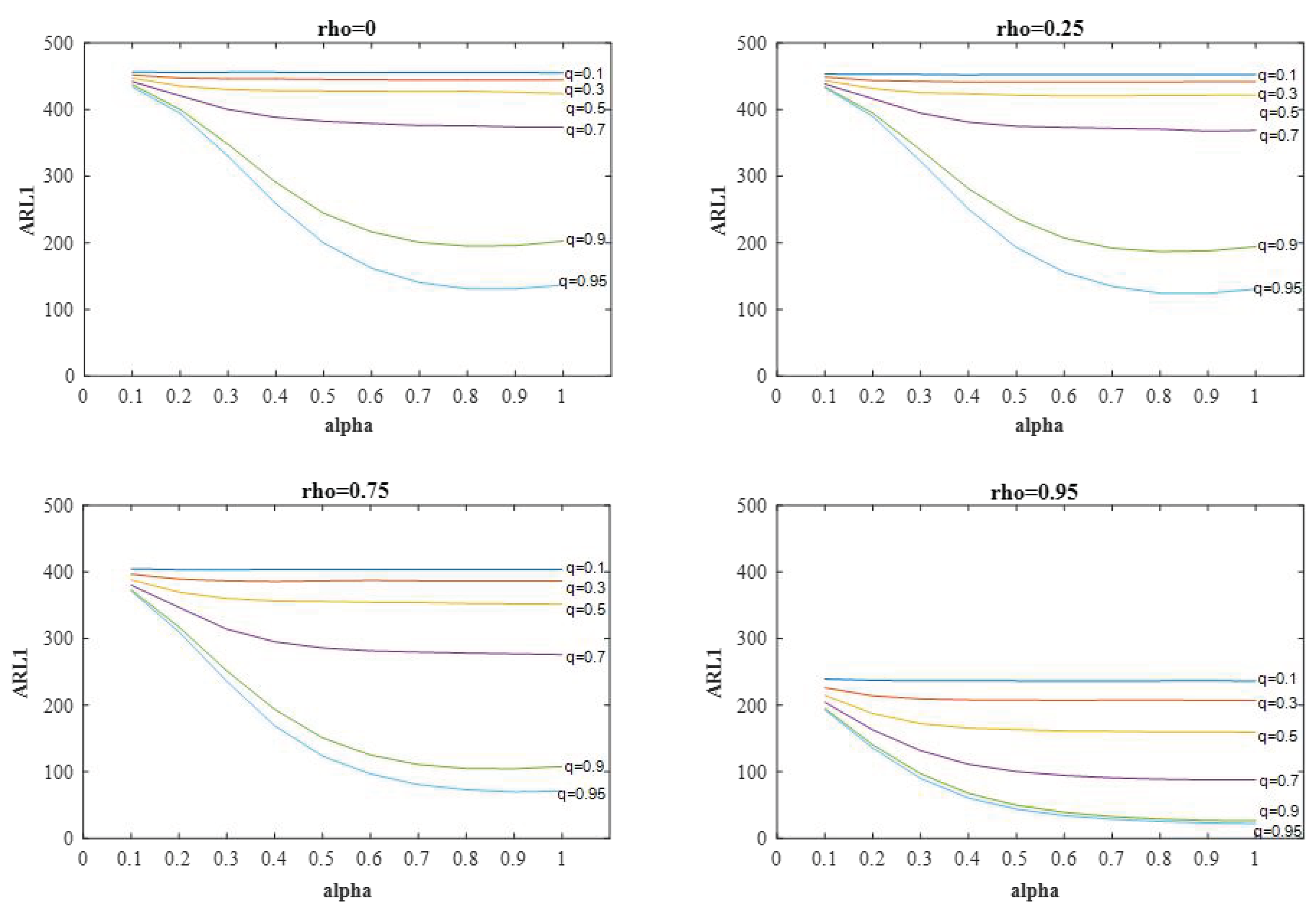
- For fixed , and , the values decrease as the value of increases. Moreover, for fixed , , and , the values tend to decrease as the value of increases. Similarly, the value is a decreasing function of when , , and are fixed.
- (4)
- The AIB-GWMA-t and AIB-EWMA-t charts uniformly perform better than the GWMA-t and EWMA-t charts, respectively. This result reveals that the use of auxiliary information enhances the performance of the GWMA-t and EWMA-t charts, especially for large values of .
- (5)
- To detect small process mean shifts, the AIB-GWMA-t chart with large and performs better than the AIB-EWMA-t chart with . However, the AIB-GWMA-t chart performs comparably to the AIB-GWMA-t chart at .
5. Illustrative Example
6. Conclusions
Author Contributions
Funding
Conflicts of Interest
Appendix A
| Input: |
| Set sample size: ; correlation coefficients: |
| Set parameters: ; |
| Set mean shifts: |
| Output: |
| Out-of-control |
| 1. Set the desired in-control |
| 2. Generate pseudo bivariate normal random numbers |
| 3. Calculate the statistic for the AIB-GWMA-t chart is by Equations (7) and (15) |
| 4. Given appropriate value of , the and can be calculated by Equation (16) |
| 5. Count the Run Length when exceeds or |
| 6. Execute 50,000 iterations of the Steps 2-5, the corresponding to the specific shift size and combination is calculated. |
| 7. Using the “Bi-Section” researching method, corresponding to the desired is obtained through repeating Steps 2–6 under in-control |
| 8. Repeat Steps 2-6 to compute under specific shift size and combination |
References
- Roberts, S.W. Control chart tests based on geometric moving averages. Technometrics 1959, 1, 239–250. [Google Scholar] [CrossRef]
- Crowder, S.V. Design of exponentially weighted moving average schemes. J. Qual. Technol. 1989, 21, 155–162. [Google Scholar] [CrossRef]
- Ng, C.H.; Case, K.E. Development and evaluation of control charts using exponentially weighted moving averages. J. Qual. Technol. 1989, 21, 242–250. [Google Scholar] [CrossRef]
- Lucas, J.M.; Saccucci, M.S. Exponentially weighted moving average control schemes: Properties and enhancements. Technometrics 1990, 32, 1–12. [Google Scholar] [CrossRef]
- Steiner, S.H. EWMA control charts with time-varying control limits and fast initial response. J. Qual. Technol. 1999, 31, 75–86. [Google Scholar] [CrossRef]
- Capizzi, G.; Masarotto, G. An adaptive exponentially weighted moving average control chart. Technometrics 2003, 45, 199–207. [Google Scholar] [CrossRef]
- Sheu, S.H.; Lin, T.C. The generally weighted moving average control chart for detecting small shifts in the process mean. Qual. Eng. 2003, 16, 209–231. [Google Scholar] [CrossRef]
- Sheu, S.H.; Chiu, W.C. Poisson GWMA control chart. Commun. Stat. Simul. Comput. 2007, 36, 1099–1114. [Google Scholar] [CrossRef]
- Sheu, S.H.; Lu, S.L. Monitoring the mean of autocorrelated observations with one generally weighted moving average control chart. J. Stat. Comput. Simul. 2009, 79, 1393–1406. [Google Scholar] [CrossRef]
- Lu, S.L. An extended nonparametric exponentially weighted moving average sign control chart. Qual. Reliab. Eng. Int. 2015, 31, 3–13. [Google Scholar] [CrossRef]
- Lu, S.L. Novel design of composite generally weighted moving average and cumulative sum charts. Qual. Reliab. Eng. Int. 2017, 33, 2397–2408. [Google Scholar] [CrossRef]
- Sheu, S.H.; Yang, L. The generally weighted moving average control chart for monitoring the process median. Qual. Eng. 2006, 3, 333–344. [Google Scholar] [CrossRef]
- Sheu, S.H.; Hsieh, Y.T. The extended GWMA control chart. J. Appl. Stat. 2009, 36, 135–147. [Google Scholar] [CrossRef]
- Huang, C.J.; Tai, S.H.; Lu, S.L. Measuring the performance improvement of a double generally weighted moving average control chart. Expert Syst. Appl. 2014, 41, 3313–3322. [Google Scholar] [CrossRef]
- Chakraborty, N.; Chakraborti, S.; Human, S.W.; Balakrishnan, N. A generally weighted moving average signed-rank control chart. Qual. Reliab. Eng. Int. 2016, 32, 2835–2845. [Google Scholar] [CrossRef]
- Aslam, M.; Al-marshadi, A.H.; Jun, C.H. Monitoring process mean using generally weighted moving average chart for exponentially distributed characteristics. Commun. Stat. Simul. Comput. 2017, 46, 3712–3722. [Google Scholar] [CrossRef]
- Riaz, M. Monitoring process mean level using auxiliary information. Stat. Neerl. 2008, 62, 458–481. [Google Scholar] [CrossRef]
- Ahmad, S.; Riaz, M.; Abbasi, S.A.; Lin, Z. On efficient median control charting. J. Chin. Inst. Eng. 2014, 37, 358–375. [Google Scholar] [CrossRef]
- Riaz, M. Control charting and survey sampling techniques in process monitoring. J. Chin. Inst. Eng. 2015, 38, 342–354. [Google Scholar] [CrossRef]
- Abbas, N.; Riaz, M.; Does, R.J.M.M. An EWMA-type control chart for monitoring the process mean using auxiliary information. Commun. Stat. Theory Methods. 2014, 43, 3485–3498. [Google Scholar] [CrossRef]
- Haq, A.; Abidin, Z.U. An enhanced GWMA chart for process mean. Commun. Stat. Simul. Comput. 2018. [Google Scholar] [CrossRef]
- Zhang, L.; Chen, G.; Castagliola, P. On t and EWMA t charts for monitoring changes in the process mean. Qual. Reliab. Eng. Int. 2009, 25, 933–945. [Google Scholar] [CrossRef]
- Celano, G.; Castagliola, P.; Trovato, E.; Fichera, S. Shewhart and EWMA t control charts for short production runs. Qual. Reliab. Eng. Int. 2011, 27, 313–326. [Google Scholar] [CrossRef]
- Celano, G.; Castagliola, P.; Fichera, S.; Nenes, G. Performance of t control charts in short runs with unknown shift sizes. Comput. Ind. Eng. 2013, 64, 56–68. [Google Scholar] [CrossRef]
- Haq, A.; Abidin, Z.U.; Khoo, M.B.C. An enhanced EWMA-t control chart for monitoring the process mean. Commun. Stat. Theory Methods. 2019, 48, 1333–1350. [Google Scholar] [CrossRef]


| 0.1 | 0.2 | 0.3 | 0.4 | 0.5 | 0.6 | 0.7 | 0.8 | 0.9 | 1.0 | ||
| 0.1 | 5.079 | 5.078 | 5.076 | 5.073 | 5.069 | 5.067 | 5.064 | 5.061 | 5.060 | 5.058 | |
| 0.2 | 5.077 | 5.071 | 5.060 | 5.053 | 5.037 | 5.029 | 5.021 | 5.007 | 5.001 | 4.993 | |
| 0.3 | 5.076 | 5.060 | 5.045 | 5.017 | 4.999 | 4.975 | 4.949 | 4.925 | 4.901 | 4.881 | |
| 0.4 | 5.075 | 5.051 | 5.016 | 4.976 | 4.939 | 4.891 | 4.850 | 4.809 | 4.766 | 4.726 | |
| 5 | 0.5 | 5.070 | 5.038 | 4.989 | 4.924 | 4.861 | 4.791 | 4.718 | 4.652 | 4.585 | 4.521 |
| 0.6 | 5.067 | 5.025 | 4.953 | 4.865 | 4.762 | 4.655 | 4.548 | 4.449 | 4.355 | 4.264 | |
| 0.7 | 5.063 | 5.008 | 4.913 | 4.782 | 4.629 | 4.474 | 4.319 | 4.180 | 4.053 | 3.943 | |
| 0.8 | 5.062 | 4.990 | 4.854 | 4.667 | 4.444 | 4.217 | 4.005 | 3.824 | 3.671 | 3.550 | |
| 0.9 | 5.060 | 4.969 | 4.787 | 4.497 | 4.154 | 3.815 | 3.526 | 3.302 | 3.145 | 3.047 | |
| 0.1 | 0.2 | 0.3 | 0.4 | 0.5 | 0.6 | 0.7 | 0.8 | 0.9 | 1.0 | ||
| 0.1 | 3.792 | 3.791 | 3.790 | 3.788 | 3.788 | 3.787 | 3.786 | 3.785 | 3.785 | 3.784 | |
| 0.2 | 3.791 | 3.787 | 3.784 | 3.780 | 3.778 | 3.774 | 3.770 | 3.765 | 3.757 | 3.754 | |
| 0.3 | 3.790 | 3.783 | 3.774 | 3.767 | 3.756 | 3.744 | 3.734 | 3.722 | 3.710 | 3.704 | |
| 0.4 | 3.790 | 3.777 | 3.768 | 3.746 | 3.728 | 3.705 | 3.689 | 3.666 | 3.647 | 3.629 | |
| 10 | 0.5 | 3.788 | 3.775 | 3.751 | 3.724 | 3.692 | 3.658 | 3.625 | 3.595 | 3.566 | 3.540 |
| 0.6 | 3.786 | 3.766 | 3.733 | 3.692 | 3.643 | 3.591 | 3.548 | 3.503 | 3.465 | 3.431 | |
| 0.7 | 3.784 | 3.758 | 3.711 | 3.643 | 3.578 | 3.511 | 3.444 | 3.385 | 3.336 | 3.296 | |
| 0.8 | 3.783 | 3.708 | 3.681 | 3.593 | 3.491 | 3.391 | 3.301 | 3.226 | 3.166 | 3.125 | |
| 0.9 | 3.782 | 3.738 | 3.645 | 3.502 | 3.339 | 3.181 | 3.059 | 2.968 | 2.910 | 2.874 | |
| 0.5 | 0.7 | 0.9 | 1.0 | 0.5 | 0.7 | 0.9 | 1.0 | 0.5 | 0.7 | 0.9 | 1.0 | 0.5 | 0.7 | 0.9 | 1.0 | 0.5 | 0.7 | 0.9 | 1.0 | |||||
| 4.861 | 4.718 | 4.585 | 4.521 | 4.852 | 4.713 | 4.584 | 4.521 | 4.861 | 4.724 | 4.590 | 4.526 | 4.854 | 4.715 | 4.580 | 4.516 | 4.861 | 4.718 | 4.585 | 4.521 | |||||
| 0.00 | 499.99 | 500.10 | 500.14 | 500.10 | 499.76 | 499.76 | 500.26 | 500.03 | 500.25 | 500.17 | 499.77 | 499.90 | 500.02 | 499.89 | 499.93 | 499.85 | 500.95 | 499.45 | 500.22 | 499.56 | ||||
| 0.10 | 427.92 | 426.79 | 425.88 | 423.93 | 421.41 | 420.66 | 421.33 | 421.76 | 404.82 | 406.46 | 406.53 | 405.86 | 355.45 | 354.09 | 352.08 | 351.54 | 163.20 | 160.85 | 160.17 | 159.38 | ||||
| 0.20 | 290.35 | 286.99 | 286.66 | 285.44 | 279.40 | 278.21 | 278.90 | 278.42 | 251.58 | 250.63 | 249.57 | 248.82 | 177.55 | 176.01 | 174.51 | 173.79 | 39.83 | 37.61 | 36.92 | 36.59 | ||||
| 0.40 | 112.49 | 110.01 | 109.08 | 108.31 | 103.94 | 102.08 | 102.07 | 101.59 | 83.63 | 81.60 | 80.88 | 80.45 | 45.47 | 43.25 | 42.46 | 42.23 | 7.51 | 6.57 | 6.09 | 5.92 | ||||
| 0.60 | 46.53 | 44.25 | 43.55 | 43.22 | 42.80 | 40.51 | 39.99 | 39.78 | 32.90 | 30.84 | 30.06 | 29.78 | 16.84 | 15.19 | 14.48 | 14.27 | 3.33 | 3.00 | 2.79 | 2.71 | ||||
| 1.00 | 13.33 | 11.80 | 11.14 | 10.92 | 12.27 | 10.86 | 10.23 | 10.05 | 9.51 | 8.35 | 7.79 | 7.61 | 5.27 | 4.63 | 4.25 | 4.13 | 1.53 | 1.50 | 1.48 | 1.48 | ||||
| 2.00 | 3.11 | 2.82 | 2.63 | 2.55 | 2.92 | 2.67 | 2.50 | 2.44 | 2.43 | 2.27 | 2.15 | 2.10 | 1.64 | 1.60 | 1.57 | 1.56 | 1.01 | 1.01 | 1.01 | 1.01 | ||||
| 0.5 | 0.7 | 0.9 | 1.0 | 0.5 | 0.7 | 0.9 | 1.0 | 0.5 | 0.7 | 0.9 | 1.0 | 0.5 | 0.7 | 0.9 | 1.0 | 0.5 | 0.7 | 0.9 | 1.0 | |||||
| 4.629 | 4.319 | 4.053 | 3.943 | 4.619 | 4.315 | 4.048 | 3.943 | 4.631 | 4.321 | 4.048 | 3.939 | 4.619 | 4.313 | 4.045 | 3.936 | 4.624 | 4.315 | 4.048 | 3.941 | |||||
| 0.00 | 500.13 | 500.27 | 500.33 | 500.16 | 499.96 | 499.66 | 499.83 | 499.73 | 500.05 | 499.81 | 500.13 | 499.54 | 500.21 | 500.13 | 500.62 | 500.05 | 500.31 | 499.99 | 499.93 | 500.05 | ||||
| 0.10 | 382.43 | 376.07 | 373.81 | 373.29 | 374.91 | 371.57 | 367.30 | 368.48 | 354.13 | 349.12 | 344.27 | 343.39 | 285.94 | 279.80 | 276.92 | 275.77 | 100.18 | 90.96 | 87.98 | 87.84 | ||||
| 0.20 | 212.28 | 203.76 | 201.07 | 200.70 | 201.70 | 193.99 | 190.96 | 191.16 | 175.02 | 165.51 | 161.61 | 161.40 | 110.43 | 101.66 | 98.75 | 98.44 | 23.65 | 18.63 | 16.66 | 16.30 | ||||
| 0.40 | 64.52 | 55.77 | 53.54 | 53.31 | 59.92 | 51.62 | 49.42 | 49.31 | 47.58 | 39.99 | 37.47 | 37.13 | 26.62 | 21.19 | 19.10 | 18.69 | 5.98 | 4.87 | 4.23 | 4.02 | ||||
| 0.60 | 27.18 | 21.62 | 19.53 | 19.14 | 25.29 | 20.06 | 17.99 | 17.67 | 20.11 | 15.69 | 13.78 | 13.35 | 11.48 | 8.97 | 7.71 | 7.36 | 3.02 | 2.68 | 2.47 | 2.39 | ||||
| 1.00 | 9.51 | 7.49 | 6.43 | 6.11 | 8.90 | 7.06 | 6.06 | 5.75 | 7.28 | 5.83 | 5.00 | 4.73 | 4.45 | 3.76 | 3.34 | 3.19 | 1.52 | 1.50 | 1.50 | 1.51 | ||||
| 2.00 | 2.85 | 2.55 | 2.36 | 2.30 | 2.70 | 2.44 | 2.28 | 2.22 | 2.30 | 2.13 | 2.02 | 1.99 | 1.62 | 1.59 | 1.58 | 1.58 | 1.01 | 1.01 | 1.01 | 1.01 | ||||
| 0.5 | 0.7 | 0.9 | 1.0 | 0.5 | 0.7 | 0.9 | 1.0 | 0.5 | 0.7 | 0.9 | 1.0 | 0.5 | 0.7 | 0.9 | 1.0 | 0.5 | 0.7 | 0.9 | 1.0 | |||||
| 4.154 | 3.526 | 3.146 | 3.047 | 4.147 | 3.520 | 3.141 | 3.044 | 4.150 | 3.522 | 3.142 | 3.042 | 4.145 | 3.521 | 3.142 | 3.042 | 4.150 | 3.522 | 3.143 | 3.045 | |||||
| 0.00 | 500.46 | 500.38 | 500.24 | 500.15 | 500.12 | 499.68 | 500.11 | 500.18 | 500.23 | 500.34 | 500.63 | 500.43 | 499.96 | 500.19 | 500.08 | 499.83 | 500.08 | 500.00 | 500.17 | 499.83 | ||||
| 0.10 | 244.10 | 200.66 | 195.69 | 202.54 | 236.52 | 191.66 | 187.69 | 194.02 | 210.36 | 166.25 | 160.91 | 166.75 | 150.93 | 111.04 | 104.44 | 108.00 | 49.88 | 32.76 | 26.94 | 26.30 | ||||
| 0.20 | 103.32 | 70.65 | 63.21 | 64.58 | 97.97 | 66.77 | 59.24 | 60.59 | 82.72 | 55.59 | 48.32 | 48.70 | 54.38 | 35.84 | 29.74 | 29.19 | 15.97 | 11.30 | 9.25 | 8.70 | ||||
| 0.40 | 34.90 | 23.09 | 18.59 | 17.71 | 32.98 | 21.86 | 17.58 | 16.76 | 27.45 | 18.44 | 14.80 | 13.99 | 17.53 | 12.28 | 10.01 | 9.39 | 5.24 | 4.37 | 3.96 | 3.84 | ||||
| 0.60 | 17.86 | 12.49 | 10.13 | 9.51 | 16.93 | 11.86 | 9.65 | 9.08 | 14.03 | 10.10 | 8.33 | 7.83 | 9.04 | 6.92 | 5.89 | 5.60 | 2.89 | 2.67 | 2.61 | 2.62 | ||||
| 1.00 | 7.75 | 6.06 | 5.25 | 5.02 | 7.35 | 5.79 | 5.05 | 4.84 | 6.18 | 5.00 | 4.44 | 4.28 | 4.07 | 3.55 | 3.31 | 3.26 | 1.54 | 1.59 | 1.70 | 1.76 | ||||
| 2.00 | 2.74 | 2.56 | 2.52 | 2.53 | 2.61 | 2.47 | 2.44 | 2.46 | 2.26 | 2.19 | 2.21 | 2.24 | 1.64 | 1.68 | 1.77 | 1.82 | 1.01 | 1.02 | 1.05 | 1.08 | ||||
| 0.5 | 0.7 | 0.9 | 1.0 | 0.5 | 0.7 | 0.9 | 1.0 | 0.5 | 0.7 | 0.9 | 1.0 | 0.5 | 0.7 | 0.9 | 1.0 | 0.5 | 0.7 | 0.9 | 1.0 | |||||
| 3.893 | 3.114 | 2.750 | 2.682 | 3.888 | 3.109 | 2.747 | 2.684 | 3.893 | 3.112 | 2.745 | 2.681 | 3.886 | 3.104 | 2.744 | 2.682 | 3.893 | 3.110 | 2.750 | 2.685 | |||||
| 0.00 | 500.18 | 499.75 | 500.21 | 500.46 | 499.56 | 499.71 | 499.93 | 500.69 | 499.56 | 500.45 | 500.63 | 500.16 | 500.01 | 499.81 | 499.93 | 500.77 | 500.40 | 500.57 | 500.25 | 500.06 | ||||
| 0.10 | 199.63 | 140.33 | 130.70 | 136.63 | 192.76 | 134.41 | 124.31 | 130.51 | 171.81 | 116.71 | 105.30 | 109.43 | 123.51 | 80.80 | 69.88 | 71.12 | 43.87 | 28.66 | 23.25 | 22.06 | ||||
| 0.20 | 85.93 | 55.11 | 45.90 | 45.06 | 81.97 | 52.56 | 43.46 | 42.80 | 70.37 | 45.10 | 36.89 | 35.90 | 47.50 | 30.95 | 25.10 | 23.91 | 15.09 | 11.13 | 9.55 | 9.10 | ||||
| 0.40 | 31.44 | 21.16 | 17.21 | 16.21 | 29.77 | 20.15 | 16.48 | 15.58 | 25.19 | 17.33 | 14.26 | 13.48 | 16.46 | 11.97 | 10.21 | 9.73 | 5.19 | 4.55 | 4.39 | 4.37 | ||||
| 0.60 | 16.75 | 12.18 | 10.33 | 9.80 | 15.89 | 11.62 | 9.92 | 9.44 | 13.34 | 10.03 | 8.68 | 8.31 | 8.76 | 7.03 | 6.36 | 6.18 | 2.90 | 2.82 | 2.94 | 3.02 | ||||
| 1.00 | 7.55 | 6.22 | 5.72 | 5.59 | 7.19 | 5.96 | 5.51 | 5.41 | 6.08 | 5.17 | 4.89 | 4.83 | 4.06 | 3.71 | 3.70 | 3.73 | 1.56 | 1.69 | 1.89 | 2.00 | ||||
| 2.00 | 2.75 | 2.71 | 2.83 | 2.91 | 2.63 | 2.61 | 2.74 | 2.84 | 2.28 | 2.32 | 2.48 | 2.59 | 1.66 | 1.77 | 1.98 | 2.09 | 1.01 | 1.04 | 1.14 | 1.24 | ||||
| 0.5 | 0.7 | 0.9 | 1.0 | 0.5 | 0.7 | 0.9 | 1.0 | 0.5 | 0.7 | 0.9 | 1.0 | 0.5 | 0.7 | 0.9 | 1.0 | 0.5 | 0.7 | 0.9 | 1.0 | |||||
| 3.692 | 3.625 | 3.566 | 3.540 | 3.688 | 3.624 | 3.564 | 3.539 | 3.688 | 3.623 | 3.565 | 3.538 | 3.685 | 3.621 | 3.563 | 3.538 | 3.688 | 3.621 | 3.563 | 3.538 | |||||
| 0.00 | 500.43 | 499.55 | 500.18 | 499.76 | 500.32 | 500.29 | 499.80 | 500.29 | 499.91 | 499.58 | 500.33 | 499.70 | 500.05 | 499.90 | 499.91 | 500.32 | 500.34 | 499.93 | 499.96 | 500.09 | ||||
| 0.10 | 267.97 | 266.89 | 268.56 | 269.64 | 257.46 | 257.98 | 258.65 | 259.83 | 226.70 | 226.83 | 229.40 | 230.53 | 155.00 | 155.70 | 157.67 | 159.09 | 33.21 | 31.40 | 31.54 | 31.91 | ||||
| 0.20 | 94.45 | 93.47 | 95.03 | 96.05 | 88.03 | 87.56 | 88.53 | 89.77 | 70.22 | 68.89 | 69.94 | 70.61 | 37.87 | 36.20 | 36.45 | 36.96 | 6.60 | 5.85 | 5.52 | 5.44 | ||||
| 0.40 | 19.47 | 17.84 | 17.58 | 17.67 | 17.95 | 16.38 | 16.06 | 16.16 | 13.79 | 12.41 | 12.07 | 12.08 | 7.46 | 6.63 | 6.28 | 6.20 | 1.79 | 1.75 | 1.73 | 1.73 | ||||
| 0.60 | 7.64 | 6.76 | 6.39 | 6.31 | 7.09 | 6.29 | 5.93 | 5.86 | 5.58 | 4.98 | 4.68 | 4.59 | 3.26 | 3.00 | 2.84 | 2.79 | 1.11 | 1.12 | 1.14 | 1.14 | ||||
| 1.00 | 2.73 | 2.55 | 2.44 | 2.40 | 2.57 | 2.42 | 2.32 | 2.29 | 2.12 | 2.04 | 1.98 | 1.97 | 1.42 | 1.42 | 1.43 | 1.44 | 1.00 | 1.00 | 1.00 | 1.00 | ||||
| 2.00 | 1.08 | 1.09 | 1.10 | 1.11 | 1.06 | 1.07 | 1.08 | 1.09 | 1.02 | 1.02 | 1.03 | 1.03 | 1.00 | 1.00 | 1.00 | 1.00 | 1.00 | 1.00 | 1.00 | 1.00 | ||||
| 0.5 | 0.7 | 0.9 | 1.0 | 0.5 | 0.7 | 0.9 | 1.0 | 0.5 | 0.7 | 0.9 | 1.0 | 0.5 | 0.7 | 0.9 | 1.0 | 0.5 | 0.7 | 0.9 | 1.0 | |||||
| 3.578 | 3.444 | 3.336 | 3.296 | 3.577 | 3.443 | 3.336 | 3.297 | 3.577 | 3.443 | 3.335 | 3.294 | 3.574 | 3.439 | 3.331 | 3.291 | 3.576 | 3.438 | 3.331 | 3.291 | |||||
| 0.00 | 499.91 | 500.22 | 500.45 | 499.63 | 500.32 | 500.38 | 500.05 | 500.25 | 500.36 | 500.12 | 499.88 | 500.39 | 500.21 | 499.81 | 499.61 | 499.65 | 499.82 | 500.03 | 500.12 | 499.96 | ||||
| 0.10 | 171.35 | 170.28 | 178.13 | 182.98 | 164.04 | 161.84 | 169.32 | 174.93 | 138.46 | 136.56 | 142.45 | 146.74 | 87.55 | 83.15 | 86.67 | 89.91 | 20.41 | 17.09 | 16.38 | 16.58 | ||||
| 0.20 | 51.56 | 46.71 | 48.01 | 49.67 | 48.50 | 43.47 | 44.63 | 46.35 | 38.89 | 34.15 | 34.47 | 35.65 | 22.81 | 19.20 | 18.55 | 18.85 | 5.57 | 4.81 | 4.41 | 4.29 | ||||
| 0.40 | 13.28 | 11.02 | 10.20 | 10.15 | 12.45 | 10.36 | 9.57 | 9.49 | 10.12 | 8.41 | 7.69 | 7.57 | 6.16 | 5.29 | 4.82 | 4.69 | 1.80 | 1.80 | 1.83 | 1.84 | ||||
| 0.60 | 6.24 | 5.36 | 4.89 | 4.75 | 5.90 | 5.08 | 4.64 | 4.52 | 4.84 | 4.26 | 3.93 | 3.81 | 3.06 | 2.83 | 2.70 | 2.66 | 1.13 | 1.17 | 1.22 | 1.26 | ||||
| 1.00 | 2.62 | 2.49 | 2.41 | 2.38 | 2.49 | 2.38 | 2.32 | 2.30 | 2.10 | 2.05 | 2.04 | 2.04 | 1.45 | 1.49 | 1.55 | 1.59 | 1.00 | 1.00 | 1.00 | 1.00 | ||||
| 2.00 | 1.10 | 1.13 | 1.18 | 1.22 | 1.08 | 1.11 | 1.15 | 1.18 | 1.03 | 1.04 | 1.07 | 1.08 | 1.00 | 1.00 | 1.00 | 1.00 | 1.00 | 1.00 | 1.00 | 1.00 | ||||
| 0.5 | 0.7 | 0.9 | 1.0 | 0.5 | 0.7 | 0.9 | 1.0 | 0.5 | 0.7 | 0.9 | 1.0 | 0.5 | 0.7 | 0.9 | 1.0 | 0.5 | 0.7 | 0.9 | 1.0 | |||||
| 3.339 | 3.059 | 2.910 | 2.874 | 3.339 | 3.061 | 2.911 | 2.875 | 3.339 | 3.065 | 2.911 | 2.876 | 3.339 | 3.061 | 2.914 | 2.876 | 3.336 | 3.057 | 2.911 | 2.878 | |||||
| 0.00 | 500.14 | 499.71 | 500.89 | 499.97 | 499.98 | 500.19 | 500.55 | 499.67 | 500.04 | 500.20 | 499.96 | 499.56 | 500.04 | 499.98 | 500.36 | 499.53 | 499.75 | 500.21 | 500.20 | 500.67 | ||||
| 0.10 | 89.90 | 73.59 | 76.23 | 81.53 | 86.01 | 70.34 | 72.33 | 77.25 | 49.87 | 59.59 | 59.83 | 63.46 | 49.87 | 39.12 | 37.56 | 38.82 | 15.72 | 12.81 | 11.51 | 11.16 | ||||
| 0.20 | 32.52 | 25.56 | 23.49 | 23.55 | 31.00 | 24.38 | 22.30 | 22.31 | 17.19 | 20.76 | 18.76 | 18.53 | 17.19 | 13.96 | 12.53 | 12.13 | 5.30 | 4.92 | 4.73 | 4.65 | ||||
| 0.40 | 11.07 | 9.33 | 8.49 | 8.20 | 10.50 | 8.93 | 8.14 | 7.87 | 5.80 | 7.66 | 7.04 | 6.82 | 5.80 | 5.31 | 5.06 | 4.96 | 1.90 | 2.08 | 2.26 | 2.34 | ||||
| 0.60 | 5.86 | 5.36 | 5.10 | 4.99 | 5.57 | 5.14 | 4.91 | 4.82 | 3.12 | 4.45 | 4.32 | 4.26 | 3.12 | 3.14 | 3.21 | 3.22 | 1.19 | 1.36 | 1.61 | 1.73 | ||||
| 1.00 | 2.70 | 2.78 | 2.89 | 2.93 | 2.58 | 2.68 | 2.80 | 2.84 | 1.55 | 2.35 | 2.50 | 2.56 | 1.55 | 1.75 | 1.95 | 2.03 | 1.00 | 1.00 | 1.04 | 1.08 | ||||
| 2.00 | 1.15 | 1.31 | 1.56 | 1.68 | 1.12 | 1.27 | 1.51 | 1.64 | 1.00 | 1.14 | 1.35 | 1.48 | 1.00 | 1.01 | 1.06 | 1.13 | 1.00 | 1.00 | 1.00 | 1.00 | ||||
| 0.5 | 0.7 | 0.9 | 1.0 | 0.5 | 0.7 | 0.9 | 1.0 | 0.5 | 0.7 | 0.9 | 1.0 | 0.5 | 0.7 | 0.9 | 1.0 | 0.5 | 0.7 | 0.9 | 1.0 | |||||
| 3.181 | 2.804 | 2.654 | 2.634 | 3.182 | 2.802 | 2.654 | 2.633 | 3.187 | 2.806 | 2.653 | 2.634 | 3.185 | 2.803 | 2.657 | 2.638 | 3.181 | 2.803 | 2.655 | 2.635 | |||||
| 0.00 | 499.85 | 499.90 | 500.00 | 499.92 | 499.81 | 500.09 | 499.76 | 499.61 | 499.88 | 500.30 | 499.66 | 499.61 | 500.13 | 500.62 | 500.63 | 500.35 | 500.15 | 500.70 | 500.46 | 499.83 | ||||
| 0.10 | 80.22 | 63.94 | 60.95 | 62.94 | 77.00 | 61.22 | 58.25 | 59.83 | 66.89 | 52.96 | 49.34 | 50.21 | 46.18 | 36.65 | 33.55 | 33.21 | 15.42 | 13.32 | 12.32 | 11.90 | ||||
| 0.20 | 30.78 | 25.07 | 22.68 | 22.07 | 29.42 | 23.94 | 21.74 | 21.10 | 25.12 | 20.66 | 18.76 | 18.15 | 16.82 | 14.38 | 13.27 | 12.80 | 5.39 | 5.36 | 5.45 | 5.44 | ||||
| 0.40 | 10.99 | 9.90 | 9.38 | 9.12 | 10.47 | 9.47 | 9.02 | 8.79 | 8.87 | 8.19 | 7.90 | 7.74 | 5.89 | 5.77 | 5.82 | 5.79 | 1.97 | 2.31 | 2.66 | 2.80 | ||||
| 0.60 | 5.94 | 5.82 | 5.86 | 5.82 | 5.66 | 5.58 | 5.65 | 5.63 | 4.80 | 4.86 | 4.99 | 5.02 | 3.21 | 3.47 | 3.76 | 3.85 | 1.22 | 1.52 | 1.88 | 2.00 | ||||
| 1.00 | 2.78 | 3.08 | 3.40 | 3.51 | 2.66 | 2.96 | 3.29 | 3.40 | 2.28 | 2.60 | 2.94 | 3.07 | 1.60 | 1.93 | 2.28 | 2.43 | 1.00 | 1.02 | 1.18 | 1.36 | ||||
| 2.00 | 1.18 | 1.46 | 1.82 | 1.95 | 1.15 | 1.41 | 1.78 | 1.92 | 1.06 | 1.26 | 1.64 | 1.80 | 1.00 | 1.03 | 1.25 | 1.45 | 1.00 | 1.00 | 1.00 | 1.00 | ||||
| The Near Optimal Design | |||||||
|---|---|---|---|---|---|---|---|
| Schemes | |||||||
| 5 | 0.00 | 0.1 | GWMA-t | 0.95 | 0.9 | 2.750 | 130.698 |
| 0.6 | EWMA-t | 0.9 | 1.0 | 3.047 | 9.506 | ||
| 2.0 | EWMA-t | 0.7 | 1.0 | 3.949 | 2.296 | ||
| 0.25 | 0.1 | AIB-GWMA-t | 0.95 | 0.9 | 2.747 | 124.315 | |
| 0.6 | AIB-EWMA-t | 0.9 | 1.0 | 3.044 | 9.081 | ||
| 2.0 | AIB-GWMA-t | 0.7 | 1.0 | 3.943 | 2.221 | ||
| 0.50 | 0.1 | AIB-GWMA-t | 0.95 | 0.9 | 2.745 | 105.297 | |
| 0.6 | AIB-EWMA-t | 0.9 | 1.0 | 3.042 | 7.828 | ||
| 2.0 | AIB-EWMA-t | 0.7 | 1.0 | 3.939 | 1.989 | ||
| 0.75 | 0.1 | AIB-GWMA-t | 0.95 | 0.9 | 2.744 | 69.875 | |
| 0.6 | AIB-EWMA-t | 0.9 | 1.0 | 3.042 | 5.599 | ||
| 2.0 | AIB-EWMA-t | 0.5 | 1.0 | 4.516 | 1.557 | ||
| 0.95 | 0.1 | AIB-EWMA-t | 0.95 | 1.0 | 2.685 | 22.064 | |
| 0.6 | AIB-EWMA-t | 0.7 | 1.0 | 3.941 | 2.395 | ||
| 2.0 | AIB-GWMA-t | 0.5 | 0.4 | 4.925 | 1.005 | ||
| 10 | 0.00 | 0.1 | GWMA-t | 0.97 | 0.9 | 2.448 | 58.390 |
| 0.6 | EWMA-t | 0.66 | 1.0 | 3.352 | 4.925 | ||
| 2.0 | GWMA-t | 0.4 | 0.4 | 3.748 | 1.076 | ||
| 0.25 | 0.1 | AIB-GWMA-t | 0.98 | 0.9 | 2.269 | 56.196 | |
| 0.6 | AIB-EWMA-t | 0.66 | 1.0 | 3.355 | 4.670 | ||
| 2.0 | AIB-GWMA-t | 0.3 | 0.4 | 3.765 | 1.056 | ||
| 0.50 | 0.1 | AIB-GWMA-t | 0.97 | 0.9 | 2.446 | 48.085 | |
| 0.6 | AIB-EWMA-t | 0.7 | 1.0 | 3.294 | 3.815 | ||
| 2.0 | AIB-GWMA-t | 0.3 | 0.3 | 3.774 | 1.017 | ||
| 0.75 | 0.1 | AIB-EWMA-t | 0.96 | 1.0 | 2.555 | 32.876 | |
| 0.6 | AIB-EWMA-t | 0.68 | 1.0 | 3.321 | 2.651 | ||
| 2.0 | AIB-GWMA-t | 0.3 | 0.3 | 3.770 | 1.000 | ||
| 0.95 | 0.1 | AIB-EWMA-t | 0.91 | 1.0 | 2.841 | 11.182 | |
| 0.6 | AIB-GWMA-t | 0.54 | 0.5 | 3.671 | 1.112 | ||
| 2.0 | AIB-GWMA-t | 0.2 | 0.3 | 3.781 | 1.000 | ||
| No. | No. | No. | No. | No. | ||||||||||
|---|---|---|---|---|---|---|---|---|---|---|---|---|---|---|
| 1 | 2.340 | 1.092 | 11 | −0.159 | −1.007 | 21 | 0.037 | −1.230 | 31 | −0.366 | −0.658 | 41 | 2.022 | −0.519 |
| −0.260 | −0.118 | 0.053 | −0.597 | 0.395 | −2.477 | −0.200 | −1.288 | 0.481 | −0.168 | |||||
| 0.652 | 0.868 | 0.206 | −0.093 | 0.310 | −0.985 | 1.370 | −1.397 | 0.432 | −0.596 | |||||
| 0.435 | −0.131 | 0.679 | 0.812 | 0.496 | −0.836 | −1.866 | 0.264 | 2.196 | 1.245 | |||||
| 1.700 | 0.010 | 0.408 | −0.576 | −0.940 | −1.936 | 0.744 | −0.579 | −0.277 | −1.524 | |||||
| 2 | 2.440 | 0.179 | 12 | 0.499 | 0.607 | 22 | 1.383 | −0.550 | 32 | 1.419 | 1.735 | 42 | −0.728 | −1.044 |
| −0.563 | −1.099 | −0.345 | 0.030 | −1.220 | −2.884 | 2.367 | 2.345 | −0.536 | −1.499 | |||||
| 1.586 | 1.341 | 0.309 | 0.111 | 1.082 | 0.349 | −0.791 | −0.602 | −0.230 | −0.374 | |||||
| −0.088 | 1.220 | −0.082 | −0.034 | 1.281 | 0.917 | −0.148 | −1.442 | 0.287 | −0.539 | |||||
| 0.627 | 1.814 | −0.556 | −0.237 | −0.043 | 0.309 | 0.677 | 1.476 | −0.307 | −0.924 | |||||
| 3 | −0.545 | 1.675 | 13 | 0.053 | 0.215 | 23 | −0.055 | −0.271 | 33 | 0.429 | 0.049 | 43 | 0.479 | 0.597 |
| 0.320 | 0.446 | 0.475 | 1.013 | 1.182 | 1.386 | −1.341 | −0.419 | 0.945 | −0.120 | |||||
| 1.334 | 0.737 | 0.260 | −1.199 | 0.074 | 1.125 | −0.042 | 0.845 | −0.040 | 0.059 | |||||
| 0.085 | −1.383 | 0.600 | 0.563 | −0.131 | −0.812 | 0.178 | −1.022 | 0.245 | −0.921 | |||||
| 1.057 | 0.584 | −0.081 | 2.508 | 0.988 | 0.984 | 1.414 | 0.533 | 0.691 | 0.928 | |||||
| 4 | −1.211 | −0.250 | 14 | −0.429 | −0.321 | 24 | 0.229 | 0.811 | 34 | 0.196 | 0.168 | 44 | −1.287 | 0.802 |
| 2.311 | 1.635 | −0.267 | 1.354 | −1.408 | 0.201 | 0.431 | −0.483 | 0.062 | −0.003 | |||||
| −0.585 | −0.237 | −1.340 | −1.035 | 0.477 | 0.778 | 2.100 | 1.264 | 0.001 | −1.385 | |||||
| 1.086 | −0.031 | 1.375 | 0.738 | −0.754 | −0.063 | 1.131 | 1.347 | −0.667 | −2.131 | |||||
| 0.481 | −1.361 | −0.342 | −2.611 | −1.081 | 1.151 | −1.040 | −1.207 | 0.159 | 0.255 | |||||
| 5 | −0.029 | 1.020 | 15 | 0.791 | −0.249 | 25 | −0.659 | −0.574 | 35 | 2.419 | −0.344 | 45 | 0.574 | 0.835 |
| 1.034 | 2.560 | −1.589 | −2.071 | 1.350 | 1.658 | −0.005 | −0.509 | −0.238 | 0.525 | |||||
| −1.428 | −0.768 | 0.525 | −0.146 | 0.417 | −0.669 | 0.103 | 0.693 | −0.422 | 0.074 | |||||
| 0.125 | −1.362 | −0.973 | −1.290 | 1.378 | −0.202 | 0.668 | 0.865 | 0.321 | −0.817 | |||||
| 0.444 | −0.944 | −0.599 | −0.767 | 0.175 | −2.290 | 1.024 | 2.418 | −0.546 | 0.065 | |||||
| 6 | 2.452 | 0.919 | 16 | −0.013 | 0.876 | 26 | 1.322 | 1.830 | 36 | −1.768 | −0.402 | 46 | 2.337 | 0.686 |
| 0.493 | −1.540 | 0.310 | −0.413 | 0.830 | 0.310 | −0.654 | 0.202 | 0.293 | 0.961 | |||||
| −0.493 | 0.372 | −1.075 | −1.048 | −0.406 | −1.277 | 1.060 | 0.726 | 0.915 | 0.994 | |||||
| 0.631 | 0.102 | 1.715 | 1.670 | 0.117 | 0.457 | 0.035 | −1.372 | 1.799 | 1.041 | |||||
| 0.977 | −0.404 | 1.004 | 0.524 | −0.564 | 0.410 | −0.207 | −0.748 | 0.697 | 1.118 | |||||
| 7 | 0.751 | −0.662 | 17 | 2.045 | 1.089 | 27 | −1.482 | −1.008 | 37 | 0.037 | −0.843 | 47 | −0.965 | 0.239 |
| 0.476 | −0.239 | −1.118 | −1.660 | 1.146 | −0.650 | 1.616 | 0.210 | −0.688 | −0.737 | |||||
| 3.065 | 0.002 | −0.834 | 0.093 | −1.352 | −0.646 | 0.588 | −0.588 | −0.199 | −1.286 | |||||
| −1.397 | −0.744 | 0.068 | −0.926 | 0.576 | −0.001 | −2.733 | −1.173 | 0.903 | 2.380 | |||||
| −0.593 | 1.603 | 0.344 | −0.293 | 1.362 | −0.715 | 1.003 | 0.786 | 0.373 | 0.701 | |||||
| 8 | −0.443 | −1.017 | 18 | 0.083 | 0.581 | 28 | 0.887 | 1.137 | 38 | −0.669 | −0.845 | 48 | 1.430 | 0.246 |
| 0.248 | 0.165 | −2.046 | −2.705 | 0.151 | −0.572 | 0.866 | 0.254 | 0.494 | −0.485 | |||||
| 0.043 | −0.375 | 0.484 | −1.689 | 0.131 | −0.612 | 0.119 | 0.637 | 1.470 | 1.104 | |||||
| −1.143 | −1.297 | 0.273 | −0.041 | −0.505 | −0.157 | −0.567 | −1.353 | 1.110 | −0.264 | |||||
| 0.185 | 0.461 | 0.793 | −0.155 | 1.076 | 0.178 | −0.907 | −0.482 | 2.529 | 1.371 | |||||
| 9 | −0.246 | −0.560 | 19 | −0.214 | 0.783 | 29 | 0.257 | 0.116 | 39 | 0.230 | 0.348 | 49 | 0.171 | 1.054 |
| −0.149 | −0.102 | −0.316 | −0.840 | 2.920 | 1.049 | 1.926 | −0.486 | 0.901 | 0.820 | |||||
| 0.805 | 0.085 | 0.851 | 0.944 | 0.390 | −0.924 | 1.521 | 0.488 | 2.287 | −1.175 | |||||
| −0.735 | 0.261 | −0.530 | −0.497 | 0.824 | −0.209 | −0.478 | −0.570 | −0.139 | −0.011 | |||||
| 0.430 | −0.649 | 1.325 | 0.408 | 1.286 | −0.797 | 0.729 | 0.922 | −0.586 | 1.066 | |||||
| 10 | −0.535 | −1.340 | 20 | −0.564 | −0.908 | 30 | 0.107 | 0.226 | 40 | −1.405 | −0.157 | 50 | 0.220 | −0.684 |
| 1.484 | 0.542 | −0.197 | −0.050 | −0.239 | −0.072 | −0.345 | −0.296 | 0.023 | −0.388 | |||||
| −0.932 | −0.799 | −1.455 | 0.047 | −3.243 | −2.441 | −0.709 | −0.750 | 1.429 | 0.920 | |||||
| 0.115 | 0.067 | 1.360 | 0.411 | −0.317 | 0.450 | −0.530 | −1.302 | −0.074 | 0.602 | |||||
| 0.373 | 0.214 | 2.273 | 1.148 | 2.015 | 0.848 | 0.654 | 1.663 | −0.697 | 0.383 |
| EWMA-t | GWMA-t | AIB-EWMA-t | AIB-GWMA-t | |||||||
|---|---|---|---|---|---|---|---|---|---|---|
| No. | ||||||||||
| 1 | 0.801 | 1.993 | 0.041 | 0.988 | 0.041 | 0.920 | 0.199 | 0.987 | 0.199 | 0.918 |
| 2 | 0.455 | 0.960 | 0.144 | 0.988 | 0.140 | 0.920 | 0.252 | 0.987 | 0.275 | 0.918 |
| 3 | 0.244 | 0.834 | 0.173 | 0.988 | 0.155 | 0.920 | 0.295 | 0.987 | 0.331 | 0.918 |
| 4 | 0.441 | 0.821 | –0.018 | 0.988 | –0.041 | 0.920 | 0.333 | 0.987 | 0.380 | 0.918 |
| 5 | –0.021 | –0.061 | 0.086 | 0.988 | 0.082 | 0.920 | 0.281 | 0.987 | 0.336 | 0.918 |
| 6 | 0.867 | 2.098 | 0.276 | 0.988 | 0.265 | 0.920 | 0.461 | 0.987 | 0.512 | 0.918 |
| 7 | 0.464 | 0.709 | 0.351 | 0.988 | 0.317 | 0.920 | 0.462 | 0.987 | 0.532 | 0.918 |
| 8 | –0.016 | –0.070 | 0.418 | 0.988 | 0.371 | 0.920 | 0.397 | 0.987 | 0.472 | 0.918 |
| 9 | 0.117 | 0.503 | 0.344 | 0.988 | 0.286 | 0.920 | 0.407 | 0.987 | 0.475 | 0.918 |
| 10 | 0.233 | 0.646 | 0.509 | 0.988 | 0.457 | 0.920 | 0.427 | 0.987 | 0.492 | 0.918 |
| 11 | 0.383 | 3.070 | 0.822 | 0.988 | 0.754 | 0.920 | 0.686 | 0.987 | 0.750 | 0.918 |
| 12 | –0.083 | –0.486 | 0.798 | 0.988 | 0.692 | 0.920 | 0.535 | 0.987 | 0.626 | 0.918 |
| 13 | –0.048 | –0.441 | 0.719 | 0.988 | 0.608 | 0.920 | 0.439 | 0.987 | 0.519 | 0.918 |
| 14 | –0.013 | –0.035 | 0.636 | 0.988 | 0.534 | 0.920 | 0.400 | 0.987 | 0.464 | 0.918 |
| 15 | 0.083 | 0.213 | 0.745 | 0.988 | 0.657 | 0.920 | 0.387 | 0.987 | 0.439 | 0.918 |
| 16 | 0.227 | 0.557 | 0.682 | 0.988 | 0.588 | 0.920 | 0.408 | 0.987 | 0.451 | 0.918 |
| 17 | 0.271 | 0.562 | 0.627 | 0.988 | 0.542 | 0.920 | 0.422 | 0.987 | 0.462 | 0.918 |
| 18 | 0.318 | 0.728 | 0.599 | 0.988 | 0.525 | 0.920 | 0.451 | 0.987 | 0.488 | 0.918 |
| 19 | 0.143 | 0.454 | 0.593 | 0.988 | 0.529 | 0.920 | 0.447 | 0.987 | 0.485 | 0.918 |
| 20 | 0.219 | 0.375 | 0.576 | 0.988 | 0.517 | 0.920 | 0.438 | 0.987 | 0.474 | 0.918 |
| 21 | 0.806 | 3.563 | 0.728 | 0.988 | 0.676 | 0.920 | 0.750 | 0.987 | 0.783 | 0.918 |
| 22 | 0.682 | 1.579 | 0.519 | 0.988 | 0.454 | 0.920 | 0.796 | 0.987 | 0.862 | 0.918 |
| 23 | 0.170 | 0.705 | 0.643 | 0.988 | 0.602 | 0.920 | 0.765 | 0.987 | 0.847 | 0.918 |
| 24 | –0.795 | –2.493 | 0.493 | 0.988 | 0.444 | 0.920 | 0.430 | 0.987 | 0.513 | 0.918 |
| 25 | 0.740 | 2.227 | 0.644 | 0.988 | 0.613 | 0.920 | 0.641 | 0.987 | 0.684 | 0.918 |
| 26 | 0.087 | 0.279 | 0.677 | 0.988 | 0.635 | 0.920 | 0.592 | 0.987 | 0.644 | 0.918 |
| 27 | 0.352 | 0.664 | 0.566 | 0.988 | 0.520 | 0.920 | 0.600 | 0.987 | 0.646 | 0.918 |
| 28 | 0.351 | 1.417 | 0.448 | 0.988 | 0.415 | 0.920 | 0.680 | 0.987 | 0.723 | 0.918 |
| 29 | 1.212 | 2.908 | 0.474 | 0.988 | 0.459 | 0.920 | 0.892 | 0.987 | 0.941 | 0.918 |
| 30 | –0.237 | –0.324 | 0.450 | 0.988 | 0.438 | 0.920 | 0.741 | 0.987 | 0.815 | 0.918 |
| 31 | 0.302 | 0.634 | 0.469 | 0.988 | 0.462 | 0.920 | 0.734 | 0.987 | 0.797 | 0.918 |
| 32 | 0.354 | 0.731 | 0.438 | 0.988 | 0.431 | 0.920 | 0.733 | 0.987 | 0.790 | 0.918 |
| 33 | 0.129 | 0.336 | 0.509 | 0.988 | 0.507 | 0.920 | 0.691 | 0.987 | 0.745 | 0.918 |
| 34 | 0.455 | 1.010 | 0.363 | 0.988 | 0.354 | 0.920 | 0.726 | 0.987 | 0.771 | 0.918 |
| 35 | 0.529 | 1.400 | 0.453 | 0.988 | 0.461 | 0.920 | 0.790 | 0.987 | 0.834 | 0.918 |
| 36 | –0.147 | –0.369 | 0.455 | 0.988 | 0.455 | 0.920 | 0.665 | 0.987 | 0.714 | 0.918 |
| 37 | 0.263 | 0.402 | 0.578 | 0.988 | 0.577 | 0.920 | 0.649 | 0.987 | 0.683 | 0.918 |
| 38 | –0.053 | –0.189 | 0.805 | 0.988 | 0.791 | 0.920 | 0.570 | 0.987 | 0.596 | 0.918 |
| 39 | 0.715 | 1.907 | 0.725 | 0.988 | 0.681 | 0.920 | 0.715 | 0.987 | 0.727 | 0.918 |
| 40 | –0.383 | –1.328 | 0.801 | 0.988 | 0.759 | 0.920 | 0.499 | 0.987 | 0.521 | 0.918 |
| 41 | 1.127 | 2.686 | 0.878 | 0.988 | 0.828 | 0.920 | 0.739 | 0.987 | 0.738 | 0.918 |
| 42 | 0.135 | 0.909 | 0.932 | 0.988 | 0.871 | 0.920 | 0.737 | 0.987 | 0.755 | 0.918 |
| 43 | 0.410 | 2.766 | 0.931 | 0.988 | 0.863 | 0.920 | 0.933 | 0.987 | 0.956 | 0.918 |
| 44 | –0.100 | –0.418 | 0.895 | 0.988 | 0.826 | 0.920 | 0.771 | 0.987 | 0.819 | 0.918 |
| 45 | –0.130 | –0.691 | 0.851 | 0.988 | 0.788 | 0.920 | 0.631 | 0.987 | 0.668 | 0.918 |
| 46 | 0.728 | 2.244 | 0.967 | 0.988 | 0.912 | 0.920 | 0.809 | 0.987 | 0.825 | 0.918 |
| 47 | –0.245 | –0.828 | 0.882 | 0.988 | 0.818 | 0.920 | 0.631 | 0.987 | 0.660 | 0.918 |
| 48 | 1.209 | 4.225 | 0.840 | 0.988 | 0.785 | 0.920 | 1.005 | 0.987 | 1.016 | 0.918 |
| 49 | 0.351 | 0.808 | 0.979 | 0.988 | 0.934 | 0.920 | 0.948 | 0.987 | 0.995 | 0.918 |
| 50 | 0.097 | 0.321 | 1.022 | 0.988 | 0.877 | 0.920 | 0.877 | 0.987 | 0.877 | 0.918 |
© 2020 by the authors. Licensee MDPI, Basel, Switzerland. This article is an open access article distributed under the terms and conditions of the Creative Commons Attribution (CC BY) license (http://creativecommons.org/licenses/by/4.0/).
Share and Cite
Chen, J.-H.; Lu, S.-L. An Enhanced Auxiliary Information-Based EWMA-t Chart for Monitoring the Process Mean. Appl. Sci. 2020, 10, 2252. https://doi.org/10.3390/app10072252
Chen J-H, Lu S-L. An Enhanced Auxiliary Information-Based EWMA-t Chart for Monitoring the Process Mean. Applied Sciences. 2020; 10(7):2252. https://doi.org/10.3390/app10072252
Chicago/Turabian StyleChen, Jen-Hsiang, and Shin-Li Lu. 2020. "An Enhanced Auxiliary Information-Based EWMA-t Chart for Monitoring the Process Mean" Applied Sciences 10, no. 7: 2252. https://doi.org/10.3390/app10072252
APA StyleChen, J.-H., & Lu, S.-L. (2020). An Enhanced Auxiliary Information-Based EWMA-t Chart for Monitoring the Process Mean. Applied Sciences, 10(7), 2252. https://doi.org/10.3390/app10072252