A United Sign Coherence Factor Beamformer for Coherent Plane-Wave Compounding with Improved Contrast

Abstract

In this study, we present a united sign coherence factor beamformer for coherent plane-wave compounding (CPWC). CPWC is capable of reaching an image quality comparable to the conventional B-mode with a much higher frame rate. Conventional coherence factor (CF) based beamformers for CPWC are based on one-dimensional (1D) frameworks, either in the spatial coherence dimension or angular coherence dimension. Both 1D frameworks do not take into account the coherence information of the dimensions of each other. In order to take full advantage of the radio-frequency (RF) data, this paper proposes a united framework containing both spatial and angular information for CPWC. A united sign coherence factor beamformer (uSCF), which combines the conventional sign coherence factor (SCF) and the united framework, is introduced in the paper as well. The proposed beamformer is compared with the conventional 1D SCF beamformers (spatial and angular dimension beamformers) using simulation, phantom and in vivo studies. In the in vivo images, the proposed method improves the contrast ratio (CR) and generalized contrast-to-noise ratio (gCNR) by 197% and 20% over CPWC. Compared with other 1D methods, uSCF also shows an improved contrast and lateral resolution on all datasets.

1. Introduction

Medical ultrasound is a widely used clinical diagnostic method due to its convenience, safety, and real-time nature. During the past few decades, the line-per-line acquisition has become the mainstream method for clinical ultrasound imaging [1]; however, the frame rate is generally limited. There are some applications which require kHz frame rates to record the tissue motion [2,3] exceeding the ability of the conventional line-per-line method.

In order to solve the low frame rate problem, ultrasound plane-wave imaging (PWI) has been applied to some advanced fields that need high frame rates [4,5] and PWI usually has low imaging quality due to insufficient transmit focusing. Montaldo et al. proposed to use several tilted-plane-wave transmissions to overcome this restriction, which is called coherent compounding [2]. Since then, coherent plane-wave compounding (CPWC) has become a promising technique in ultrafast ultrasound imaging [2,6].

However, there is a tradeoff between the frame rate and image quality in CPWC: the higher the number of angles to obtain an image, the better the image quality but the lower the frame rate [6]. In theory, the frame per second (fps) of one-angle CPWC could reach 15,000 Hz at a depth of 5 cm, while it drops down to 1500 Hz using 11-angle CPWC. Thus, it is important to improve the image quality without increasing the number of angles.

Montaldo et al. used the delay-and-sum (DAS) algorithm for image reconstruction in each plane wave, which is now widely accepted as a standard reconstruction method for CPWC [2,6]. DAS uses the simple addition of the channel signal data in the delay line. It does not take into account signal coherence and can only obtain limited imaging quality. In order to improve the spatial and contrast resolution, various adaptive beamformers have been proposed besides the conventional DAS method. The minimum variance beamforming and coherence-based beamforming are two important parts of the beamformers [7]. Capon [8] proposed the minimum variance (MV) and in 1969 and Asl [9] proposed eigenspace-based minimum variance (ESBMV) beamforming on the basis of MV. The minimum variance beamforming could achieve better resolution than DAS, but its computational amount is also large. Meanwhile, the coherence-based beamforming is an important part of the adaptive beamformers as well [7], which could increase detail resolution and contrast with less computational amount. Recently, many beamformers based on the machine learning [10] and compressed sensing [11] also made much progress.

The coherence-based beamforming is still of great significance today because of its ease of calculation and improved image quality. Previous theory on the coherence based beamformer of medical ultrasound signals was adapted from the van Cittert Zernike (VCZ) theorem to describe the spatial coherence of ultrasound radio-frequency (RF) signal [12]. It works as a spatial filter to enhance or attenuate the signal from the location information. Mallart and Fink first introduced the coherence factor beamformer in 1994 [13]. Liu used this theory to develop a phase aberration correction method [14,15]. Subsequently, a variety of techniques utilizing spatial coherence have been developed [16,17,18,19]. Among these spatial coherence beamformers, the Phase Coherence Factor (PCF) beamformer and Sign Coherence Factor (SCF) beamformer were first introduced by Camacho based on the analysis of the phase diversity of the aperture data [18]. For phase quantization, SCF can be treated as the ‘simplified’ version of PCF.

In addition to the spatial method, the angular theory could also improve image quality. The angular coherence theory has been proposed as an extended form of the van Cittert-Zernike theorem [20]. It was first introduced by Walther et al. in the context of optics [21]. In recent years, Li introduced the angular coherence theory in medical ultrasound imaging and analyzed the autocorrelation function of the CPWC signal [20]. Furthermore, Li and Wang further applied the angular coherence theory to new beamformers [20,22]. The angular beamformers operate on the DAS data instead of the RF channel data. Thus, they significantly reduce the amount of calculation in comparison with the spatial beamformers.

However, the spatial and angular coherence theory use only their own single-dimensional-coherence character of RF data, which limits the image quality of CPWC. In this study, we proposed a new united sign coherence factor (uSCF) method that unites the spatial and angular coherence characters to further improve image quality. The rest of this paper is organized as follows. In Section 2, the conventional methods (spatial-SCF and angular-SCF methods) are introduced, and the new united beamforming framework and uSCF beamformer are presented. In Section 3, we introduced the acquisition parameters and the evaluation metrics for the study. In Section 4, the performance of the new beamformer is shown compared with the conventional beamformers using simulation, phantom, and in vivo study. The analysis about the performance of the beamformers is discussed and explained in Section 5. The conclusion is in Section 6.

2. Methods

2.1. Proposed Coherent Plane-Wave Compounding

In CPWC, data are acquired by transmitting multiple tilted plane-waves and compounding tilted receive-signals over the entire imaging region. The process is shown in Figure 1. The x-direction is parallel to the transducer array, and z is the depth direction of the imaging medium.

We defined ${\alpha }_i$ as the inclination angles of a set of N plane waves and each point (x,z) of every transmitted-angle (${\alpha }_i$) image can be expressed as [5]

$$X_c^i(x,z)={\displaystyle \sum _{\mathrm{j}=1}^{M}RF(x_j,\tau (x,z,x_j))},$$

(1)

where M is the element number of the aperture which depends on the F-number and $x_j$ is element position. $X_c^i$ is the ultrasound image of ${\alpha }_i$ (i = 1,2,3…N). The delay τ changes with different angles and it can be expressed as:

$$\tau (x,z,x_j)=(zcos{\alpha }_i+xsin{\alpha }_i)/c+\sqrt{(z^2+{(x-x_j)}^2)}/c.$$

(2)

Let $X_c$ be the CPWC image of the point (x,z). It can be given as [2]:

$$X_c(x,z)=\frac{1}{N}{\displaystyle \sum _{\mathrm{i}=1}^N{X}_c^i(\mathrm{x},\mathrm{z})}=\frac{1}{N}{\displaystyle \sum _{\mathrm{i}=1}^N{\displaystyle \sum _{\mathrm{j}=1}^{M}RF(x_j,\tau (x,z,x_j))}},$$

(3)

where N is the number of tilted-angles.

We can replace the signal position index (x,z) to the discrete-time index k. After distance transform, the RF signals for a specific point in (3) can be shown in a 2D matrix X(k) [23]

$$X(\mathrm{k})=\left(\begin{array}{ccc}{x}_{1,1}(\mathrm{k})& \dots & x_{1,M}(\mathrm{k})\\ ⋮& \ddots & ⋮\\ x_{N,1}(\mathrm{k})& \cdots & x_{N,M}(\mathrm{k})\end{array}\right),$$

(4)

where $x_{i,j}(\mathrm{k})$ is the RF signal received by the element $j$ at the tilted angle ${\alpha }_i$. In the DAS method, we could obtain the $X_c^i$ (1) and $X_c$ (3) in the discrete form:

$$X_c^i(\mathrm{k})=\frac{1}{M}{\displaystyle \sum _{\mathrm{j}=1}^M{x}_{i,j}(\mathrm{k})},$$

(5)

$$X_c(\mathrm{k})=\frac{1}{N}{\displaystyle \sum _{\mathrm{i}=1}^N{X}_c^i}(\mathrm{k})=\frac{1}{MN}{\displaystyle \sum _{i=1}^N{\displaystyle \sum _{\mathrm{j}=1}^M{x}_{i,j}(\mathrm{k})}}.$$

(6)

More details of CPWC can be found in [2]. Montaldo et al. applied the DAS to CPWC, and it was accepted as a standard method. The framework is shown in Figure 2a.

Conventional coherence beamformers processes to the rows or the columns of $X_c$ in Equation (6). The operations in the rows and columns respectively focus on the signals within each plane-wave transmission and superposition signals at different angles. To differentiate the two conventional ways, we name them spatial beamformer and angular beamformer. In Section 2.2, we will describe the proposed spatial and angular SCF beamformer applied to CPWC.

2.2. Proposed Spatial and Angular SCF Beamformer

Conventional SCF splits the phase range into two parts according to the sign of the signal [18]. RF signals could be approximately identified relevant if their phases all belong to a certain part. The SCF can be calculated as:

$$SCF(k)=1-\sqrt{1-{\left[\frac{1}{M}{\displaystyle \sum _{j=1}^M{b}_j(\mathrm{k})}\right]}^2},$$

(7)

where b is the sign bit of the aperture data and M is the element number of the aperture.

Conventional SCF relies on the phase coherence among the receiving backscattered signals at each element of the aperture, which is caused by the distance difference from the scatter point to each of these elements [24]. It also simplified the calculation of phase coherence by using the sign bit of RF data. As it focuses on the similarity between the channel signals received on transducer elements which differ in space, conventional SCF acts as a spatial filter. To emphasize the characteristics of its attention to spatial information, we name it spatial SCF (sSCF).

Based on the CPWC beamforming in Section 2.1, the spatial sign bit b of the RF signal data must be in matrix form as:

$$b_{i,j}(\mathrm{k})=\{\begin{array}{ccc}-1& if& x_{i,j}(\mathrm{k})<0\\ 1& if& x_{i,j}(\mathrm{k})\ge 0\end{array}.$$

(8)

The sSCF focuses on the information at the aperture within every angle, so the standard deviation $\sigma$ of sSCF is

$${\sigma }_i(k)=\sqrt{1-{\left(\frac{1}{M}{\displaystyle \sum _{j=1}^M{b}_{i,j}(\mathrm{k})}\right)}^2},$$

(9)

where the subscript $i$ of ${\sigma }_i$ means every $X_c^i$ has its own $\sigma$. And the beamformer weights $sSC{F}_i\left(\mathrm{k}\right)$ and final output $Y_s(\mathrm{k})$ for CPWC could be expressed as

$$sSC{F}_i\left(k\right)=1-{\sigma }_i=1-\sqrt{1-{\left(\frac{1}{M}{\displaystyle \sum _{j=1}^M{b}_{i,j}(\mathrm{k})}\right)}^2},$$

(10)

$$Y_s(\mathrm{k})=\frac{1}{N}{\displaystyle \sum _{i=1}^{N}sSC{F}_i\left(k\right)X_c^i}(\mathrm{k}),$$

(11)

where the subscript S of $Y_s(\mathrm{k})$ means ‘spatial’. Its flow diagram is shown as Figure 2b.

The sSCF beamformer measures the spatial coherence of the RF data. Based on the angular coherence presented in [20], the angular SCF (aSCF) beamformer can be proposed as well.

The aSCF beamformer operates on superposition data rather than postsummed RF data. The angular sign bit of the CPWC data can be shown as:

$$b_i(\mathrm{k})=\{\begin{array}{ccc}-1& if& X_c^i(k)<0\\ 1& if& X_c^i(k)\ge 0\end{array}.$$

(12)

The aSCF focuses on the information with the angles, so the standard deviation of $b_i(\mathrm{k})$, aSCF and output $Y_a(\mathrm{k})$ are shown as:

$$\sigma (k)=\sqrt{1-{\left(\frac{1}{N}{\displaystyle \sum _{i=1}^N{b}_i(\mathrm{k})}\right)}^2},$$

(13)

$$aSCF\left(k\right)=1-\sigma =1-\sqrt{1-{\left(\frac{1}{N}{\displaystyle \sum _{i=1}^N{b}_i(\mathrm{k})}\right)}^2},$$

(14)

$$Y_a(\mathrm{k})=\frac{1}{N}aSCF(\mathrm{k}){\displaystyle \sum _{i=1}^N{X}_c^i(\mathrm{k})}.$$

(15)

The subscript a of $Y_a(\mathrm{k})$ means ‘angular’ and its framework is described in Figure 2c.

2.3. United CF-based Beamforming Framework

The sSCF and aSCF method both use the signal coherence of the RF data to weight the coherent sum output. Omitting the same ‘sign coherence factor’, their differences are reflected in the ‘spatial’ framework and ‘angular’ framework shown in Figure 2b,c.

The spatial method calculates the coherence factor within every row of the matrix X(k) and the angular method obtains the factor after adding the entries in each row along the remaining column. Ultrasound backscattered signals contain coherence information in both the spatial and angular dimension, so the spatial framework and the angular framework could be combined to produce a united adaptive beamforming framework. We propose a new framework utilizing both the spatial coherence and angular coherence. The new framework unites the two kinds of coherence together. In the framework, all the elements of the matrix represent the information of the corresponding point (x,z), and the coherence among them should be evaluated directly. So, the united CF-based beamforming framework acts as a united 2D filter in the spatial and angular dimension. Its schematic diagram is shown as Figure 2d.

By the new united framework, the beamforming weight factor $w_u$ could be calculated by the postsummed data matrix before DAS of all angles and applied to the additional result of the DAS.

Based on the united framework, the factor $w_u$worked as:

$$Y_u(k)=\frac{1}{N}{w}_u(k){\displaystyle \sum _{i=1}^N{X}_c^i(k)},$$

(16)

where $w_u$ is the coherence factor of the matrix of all information (both in spatial and angular dimension) from the point.

2.4. United SCF Beamformer

Based on the united framework presented here, we propose the united sign coherence factor beamformer (uSCF). The uSCF combines the sign coherence factor [18] and united framework (Section 2.3). The united framework allows the uSCF beamformer to make full use of phase information in both the spatial and angular dimensions.

The matrix X(k) in Equation (4) is the received RF signal from the point (x, z), which contains all information in both spatial and angular dimensions. Based on the SCF theory in Section 2.1, the 2D sign phase bit $b_{i,j}$ uses the same representation as (8), where i and j are the index of angles and elements in transducer aperture, respectively. Different from the $\sigma$ in aSCF, the standard deviation of $b_{i,j}$ in uSCF is

$$\sigma (k)=\sqrt{1-{\left(\frac{1}{MN}{\displaystyle \sum _{j=1}^M{\displaystyle \sum _{i=1}^N{b}_{i,j}(k)}}\right)}^2},$$

(17)

where the square value of the averaged sign data is inversely proportional to ${\sigma }^2$, which represents the similarity of the matrix X(k). It is obvious that ${\sigma }^2$ ranges from 0 (all the elements are same) to 1 which is also similar to the sSCF and uSCF. The uSCF can be defined as:

$$uSCF(\mathrm{k})=1-\sigma =1-\sqrt{1-{\left(\frac{1}{MN}{\displaystyle \sum _{j=1}^M{\displaystyle \sum _{i=1}^N{b}_{i,j}(k)}}\right)}^2}$$

(18)

In this expression, we only consider the $x_{i,j}$’s polarities. Similar to the 1D beamformer, uSCF reaches to its max (one) when all discrete signal data belongs to the positive or negative classification interval. Correspondingly, uSCF takes the minimum (zero) when all discrete signal data could be divided equally into two intervals. Based on (16), the final output of uSCF could be shown as:

$$Y_u(\mathrm{k})=\frac{1}{N}uSCF(\mathrm{k}){\displaystyle \sum _{i=1}^N{X}_c^i(\mathrm{k})}.$$

(19)

2.5. Implementation Summary of Algorithm

The implementation summary of the beamforming uSCF is shown in this section. The process also corresponds to Figure 2d.

(1) Calculate the delay time of each pixel in the image according to the position of the pixel and the angle of the tilted plane wave. The matrix X(k) (4) could be obtained after the time delay calculation.

(2) Calculate the average value of the matrix X(k) to get the DAS result. The average value is also the CPWC result shown in (6).

(3) According to the positive and negative, transform X(k) into its sign matrix. Calculate the united sign coherence factor using (17) and (18).

(4) Apply the result of step 3 as the weight value to the result of step 2 on the original echo data as in (19).

(5) Repeat step 1 to 4 for each pixel of the beamformed image to get the final result.

3. Acquisition Parameters and Evaluation Metrics

3.1. Acquisition Parameters

We compare the performance of the beamformers on imaging data from the simulation, phantom and in vivo data.

The simulated datasets were generated with Field II [25,26]. It contains two simulated datasets to evaluate the lateral resolution and contrast, respectively. The two datasets are both simulated with a 128-element probe, and the central frequency is 7.81 MHz. Each dataset contains 11 tilted plane-waves linearly distributed between −18° and +18° (angles number = 11).

The mimicking phantom and in vivo datasets were acquired by an ultrasound imaging system (Vantage, Verasonics, WA, USA) with a L11-5V transducer. The mimicking phantom has isolated scatters and an anechoic cyst. The in vivo data we used is from the right-side neck of a healthy 28-year-old volunteer. Each set also contains data acquired by 11 tilted plane-waves distributed from −18° to +18° (angles number = 11). The simulation and the experiment parameters are the same, and all the imaging parameters are shown in

Table 1. Experimental imaging parameters.

Parameter	Value
Pitch	0.3 mm
Element width	0.27 mm
Number of elements	128
Transmit frequency	7.81 M [Hz]
Bandwidth	4.8M~10.8 M [Hz]
Sampling frequency	30 M [Hz]
F-number	1.75
Frame rate	50 Hz

.

3.2. Evaluation Metrics

For spatial resolution, we use the criteria full width at half maximum (FWHM, −6 dB beam width) [27] and point targets to analyze the performance. For contrast resolution, we use anechoic objects to analyze its contrast ratio (CR) [27] and generalized contrast-to-noise ratio (gCNR) [28].

Spatial resolution could be measured through the response to individual scatters of the beamformed image. Because SCF mainly improves the lateral resolution given by Rayleigh criterion [18], we use the FWHM in the lateral direction to evaluate the performance of each beamformer. To be more specific, a lower FWHM means a narrower lobe and higher spatial resolution.

To measure the contrast resolution, the criteria CR and contrast-to-noise ratio (CNR) are often used. They are measured using the following equation [27]:

$$CR=20\hspace{0.17em}{\log }_{10}(\frac{{\mu }_{ROI}}{{\mu }_B}),$$

(20)

$$CNR=20{\log }_{10}(\frac{{\mu }_{ROI}-{\mu }_B}{\sqrt{{{\sigma }_{ROI}}^2+{{\sigma }_B}^2}}),$$

(21)

where $\mu$ is the added value of the beamformed envelope signal over a certain region and $\sigma$ is the standard deviations of the signal. The subscript ROI and B represents the region of interest and background, respectively. However, Nguyen et al. showed that the metric CNR has the opposite trend compared with the spatial resolution, which means it may not be an effective independent judgment criterion for contrast resolution [29]. Molares et al. also showed CNR’s characteristic which is susceptible to dynamic range [28]. Thus, we use gCNR to replace CNR. gCNR is resistant to dynamic range alterations [28], which could help us exclude the difference in dynamic range. It is given by the equation:

$$\mathrm{g}CNR=1\text{-}OVL,$$

(22)

where OVL is the overlap area between the two probability distributions of the region of interest and background [28].

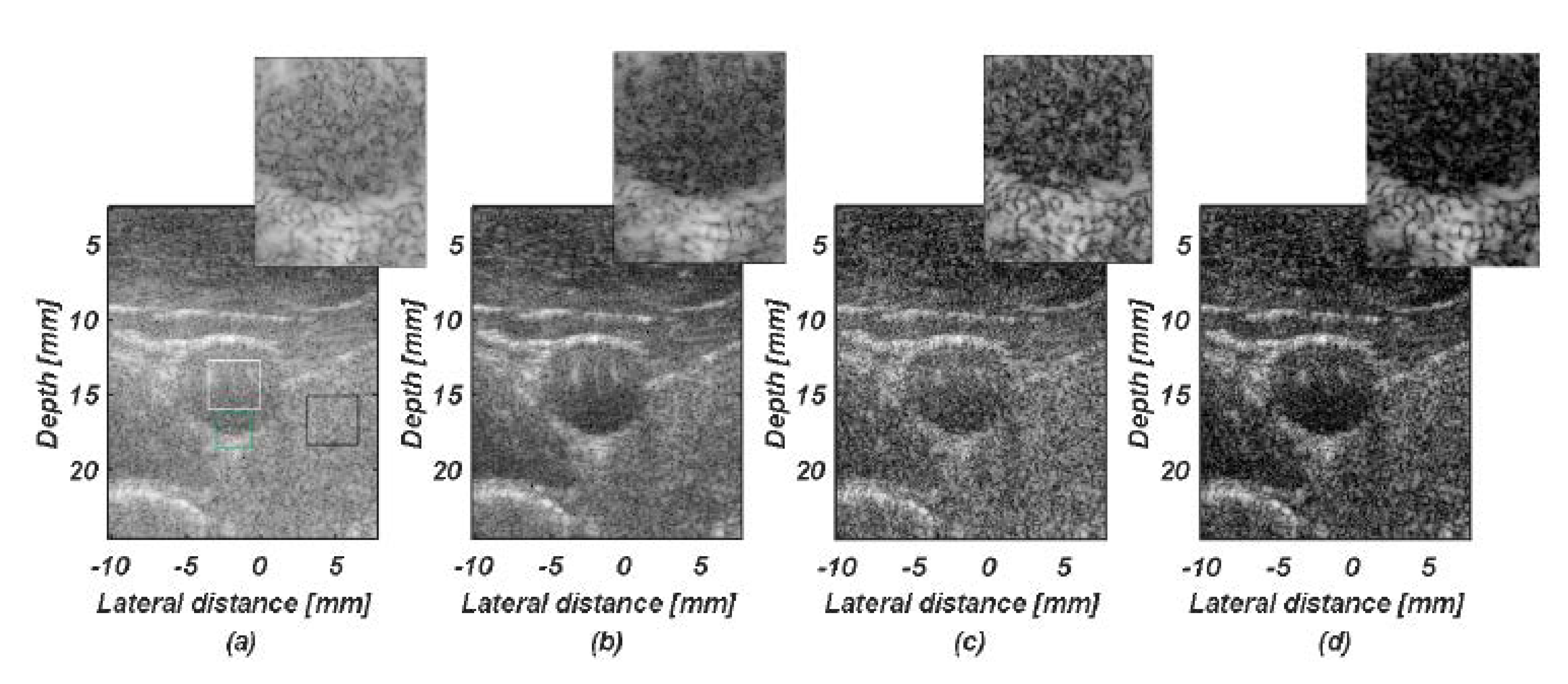
4. Imaging Data and Results

4.1. Simulation Study

We applied the beamformers to the point-simulation dataset and anechoic-simulation dataset. The two datasets are designed to evaluate lateral resolution and contrast resolution performance, respectively.

Figure 3a–d shows the simulated point target images created by different methods. Five-point targets are simulated along the depth direction in the image horizontal center, ranging from 5 to 20 mm. There is also one set of nine equally spaced point-targets horizontally located at depths of 12.5 mm.

In Figure 3a, the original image is shown with the evident grating lobe artifacts. Comparing with DAS, all the beamformers show their ability to reduce the artifacts, but the sSCF and aSCF beamformers still exhibit some artifacts in the near field. The proposed uSCF beamformer outperforms other methods with visually clean background.

We selected two-point targets for envelope signal presentation in Figure 4 and we could analyze the lateral response of different beamformers graphically. The two points are in the center of the image at depths of 10 and 15 mm. It shows that all the SCF-based beamformers help to increase the lateral resolution compared with DAS, and the uSCF has the narrowest responses both in the near and far field. It improves lateral resolution and decreases the side lobe level over the best of the conventional methods. In order to quantify the lateral resolution, the averaged FWHMs of all the points are summarized in

Table 2. Contrast performance from simulation.

Beamformer	FWHM (mm)	25 mm CR (dB)	25 mm gCNR	35 mm CR (dB)	35 mm gCNR
$\mathrm{DAS}$	0.1397 ± 0.0025	9.12	0.63	11.45	0.75
$\mathrm{sSCF}$	0.1105 ± 0.0045	13.88	0.70	15.70	0.79
$\mathrm{aSCF}$	0.1068 ± 0.0173	15.15	0.70	17.85	0.78
$\mathrm{uSCF}$	0.0966 ± 0.0030	20.77	0.74	22.48	0.82

. Compared with other SCF-based beamformers, the uSCF image has the least artifacts and the best resolution at all depths.

The anechoic-simulation dataset for evaluating the contrast resolution is shown in Figure 3e–h. The two simulated circular anechoic cysts are at a depth of 25 mm (3-mm-radius) and 35 mm (2-mm-radius) with scatters surrounding them. Figure 3e–h shows the cyst images with different beamformers, respectively.

As shown in Figure 3e–h, in contrast to DAS, the spatial and angular methods both make the cyst more distinguished, the CRs produced with aSCF and sSCF are numerically approximate, but the sSCF beamformer shows a clearer speckle. Meanwhile, with the uSCF shown in Figure 3h, the noise inside the cyst is reduced more in comparison to the other beamformers. The lesion also shows a higher contrast over the other beamformers. The lesion CRs and gCNRs at different depths are both shown in Table 2. Compared with DAS, uSCF improves CR more than 100% and gCNR more than 10%. It also shows the best contrast resolution among the SCF-based beamformers.

4.2. Phantom Study

We applied the beamformers to experimental data acquired with a gelatin-phantom with five nylon targets and an anechoic cyst. The nylon targets and anechoic cyst are designed to evaluate lateral resolution and contrast resolution performance, respectively. Figure 5 shows the different SCF based beamformers results, and all beamformers are applied to the same data.

The images about the lateral resolution result are shown in Figure 5a–d. The horizontal distances of the center of the point target line are 4, 3, 2, and 1 mm. In the phantom study, images generated by the SCF-based beamformers also show an enhanced effect over DAS. Similar to the simulation results, uSCF still performs best as the boundary between every two points is clearest. For each beamformer, we measured the lateral resolution over all five nylon targets and the average result is in

Table 3. Contrast performance from phantom and in vivo.

Beamformer	FWHM (mm) (phantom)	CR (dB) (phantom)	gCNR (phantom)	CR (dB) (in vivo)	gCNR (in vivo)
$\mathrm{DAS}$	0.3192 ± 0.0150	11.50	0.39	3.57	0.58
$\mathrm{sSCF}$	0.2304 ± 0.0090	16.98	0.54	7.73	0.67
$\mathrm{aSCF}$	0.2484 ± 0.0180	16.68	0.53	5.75	0.62
$\mathrm{uSCF}$	0.2028 ± 0.0090	22.17	0.61	10.59	0.70

.

To show the performance of the SCF-based beamformers in more details, Figure 6 plots the lateral responses to the two rightmost point targets. As expected, the uSCF achieves a higher lateral resolution and lower side lobes, which means better ability to distinguish two close-up points.

Figure 5e–h shows the images of an experimental phantom with a cyst (4 mm in diameter) suspended against the speckle background. Images are shown with the same dynamic range using different methods. These images show noticeable improvement in contrast resolution for the SCF-based beamformers compared with DAS. The cyst is much cleaner with a much sharper edge for uSCF. We also take the white region as ROI and the black as background to analyze the images’ CR and gCNR. The results are also shown in Table 3. Compared with other methods, uSCF could offer improvements to CR and gCNR better than the best performance of other beamformers, which means the uSCF image has better ability in distinguishing cyst from background. The uSCF improves CR (92%) and gCNR (56%) over DAS, and it also improves CR (30%) and gCNR (12%) over the best of conventional methods (sSCF).

4.3. In Vivo Study

The data of biological tissues shows they have their own characteristics because of the complex physiological structure, so it is necessary to test the new beamformer in vivo. We used ultrasound data from the carotid artery of a healthy person by Vantage to evaluate all the beamformers. Figure 7 shows the ultrasound images of the carotid artery using different beamformers.

The artery is shaped as a round structure in the figure, and it performed as an anechoic region because of the lumen. We take the artery as ROI (white box) and surrounding tissues as background (black box). The CR and gCNR result of the artery region for each beamformer is also reported in Table 3. uSCF provides the CR and gCNR improvement of above 197% and 20%, respectively. It also improves CR (36%) and gCNR (4%) over the best conventional method.

Each image is also shown with a magnified view of the region enclosed by the green square (shown in the upper-right corner). The boundary of the artery is sharper with uSCF, which is meaningful for ultrasound diagnosis.

5. Discussion

5.1. Comparision of SCF-Based Beamformers Performance

The image results (simulation, phantom and in vivo) show that the uSCF beamformer offers improvements over the conventional DAS, sSCF and aSCF beamformers. To further illustrate the proposed method, we present the CR and gCNR in simulation (35-mm-depth cyst) as a function of the number of transmitted plane waves, varying from 1 to 11. As shown in Figure 8, both the CR and gCNR increase with the number of angles for all the methods, and the uSCF performs best at all numbers of the angles. We also note that uSCF and aSCF ‘degenerate’ to the same as sSCF and DAS, respectively, under the premise of single-angle plane waves (0°). It is due to the lack of angular coherence, which could also be deduced from the Equations (14) and (18).

The improvements of uSCF could be explained by two reasons. First, uSCF uses both the spatial coherence factor (sSCF) and angular coherence factor (aSCF). The two coherence factors could be combined to further improve image quality. Second, uSCF calculates the coherence factor from all the elements in $X(\mathrm{k})$ (4), which helps to improve the accuracy of the estimation. The cyst results in the simulation, phantom and in vivo show that the uSCF beamformer offers improvements to suppress noise over the other beamformers.

SCF-based beamformers are obtained from the phase diversity to discriminate the signals from the noise. The simulation and experimental results show that the SCF-based beamformers offer significant improvements over DAS.

The improvements of sSCF mainly come from the spatial coherence within each plane wave. Based on the acoustic reciprocity theory, Bottenus et al. proved its validity [19]. However, the sSCF ignores the angular coherence among the different transmits, thus causing its performance to be lower than the uSCF.

The images produced with an aSCF beamformer on simulation and experiment data show good agreement with those produced with the sSCF beamformer, which is similar to the results of Li [20]. Based on the acoustic reciprocity, Li proved its validity with respect to the angular coherence of ultrasound, also significantly reducing computational costs.

However, the decrease in the improvement effect of aSCF from the in vivo data may be explained by the phase shift caused by tissue motions. There will be a longer time interval between the first and last plane wave of a compounded image than the time between the ‘adjacent’ plane wave. The biological motion may cause phase shift during the time [30], and it causes lower cross-correlation coefficient values between different angles. Because aSCF only use the coherence among the angles, it performs worse than the sSCF and uSCF. Meanwhile, uSCF takes use of both the angular and spatial coherence, and it still performs best when the angular coherence has limited promotion effect. The result of in vivo data proves the effectiveness and robustness of uSCF from the side.

These results clearly suggest that the SCF beamformers in CPWC should be calculated from data before superposition among all the angles, which is in the approach of uSCF.

5.2. Computational Complexity

To determine the computational complexity of the SCF-based beamformers, let M denote the number of elements in the aperture, and N denote the number of the tilted angles as mentioned in Section 2. For each sample of the RF image, the computational complexity of the beamformers is shown in

Table 4. Computational complexity for one sample.

Beamformer	Addition Operations	Multiplication Operations
DAS	MN	0
$\mathrm{sSCF}$	2MN	N
$\mathrm{aSCF}$	MN+N	1
$\mathrm{uSCF}$	2MN	1

. The number of floating operations in uSCF is between sSCF and aSCF.

As reported in [18], the sign bit factor and aperture data can be calculated separately in real time. Moreover, the GPU platforms can also be used to execute the beamforming for plane wave imaging and factor computation because of the parallelism of the calculation. Thus, the uSCF and aSCF could get the same frame rate. Since real-time visualization is not our primary goal, the RF signals were calculated offline on CPU in our study.

6. Conclusions

In this study, we have presented a united SCF beamformer that is designed to integrate with CPWC. When applied to data from CPWC, the uSCF beamformer calculates from the data before superposition among the angles. Thus, it makes full use of the phase information compared with the spatial beamformer (sSCF) and angular beamformer (aSCF).

Through the results on imaging data, the uSCF offers significant improvements over CPWC and conventional SCF beamformers (sSCF and aSCF) in both lateral resolution and contrast resolution by simulation, phantom, and in vivo experiments. For simulated images, the CR improvements are over 100%. In experimental images, the maximum improvements of the lateral full width at half maximum (FWHM), CR and gCNR are 35%, 92% and 56%, respectively. In the in vivo experiment, the CR and gCNR of the artery is increased by 197% and 20%. The performance of uSCF also proves, to some extent, the validity of the united beamforming framework in uSCF.

The uSCF also needs further investigation. A proper threshold should be considered to improve the robust of the united approach. Because all the elements in the matrix weight equality in the coherence factor method, the performance of weight factor could also be influenced by very few elements.

References

1. Szabo, T.L. Diagnostic Ultrasound Imaging: Inside Out; Academic Press: Cambridge, MA, USA, 2004. [Google Scholar]
2. Blanco-Andujar, C.; Ortega, D.; Southern, P.; Nesbitt, S.A.; Thanh, N.T.K.; Pankhurst, Q.A. Coherent plane-wave compounding for very high frame rate ultrasonography and transient elastography. IEEE Trans. Ultrason. Ferroelectr. Freq. Control 2009, 56, 489–506. [Google Scholar]
3. Bercoff, J.; Montaldo, G.; Loupas, T.; Savery, D.; Mézière, F.; Fink, M.; Tanter, M. Ultrafast compound Doppler imaging: Providing full blood flow characterization. IEEE Trans. Ultrason. Ferroelectr. Freq. Control 2011, 58, 134–147. [Google Scholar] [CrossRef] [PubMed]
4. Couture, O.; Fink, M.; Tanter, M. Ultrasound contrast plane wave imaging. IEEE Trans. Ultrason. Ferroelectr. Freq. Control 2012, 59, 2676–2683. [Google Scholar] [CrossRef] [PubMed]
5. Tanter, M.; Fink, M. Ultrafast imaging in biomedical ultrasound. IEEE Trans. Ultrason. Ferroelectr. Freq. Control 2014, 61, 102–119. [Google Scholar] [CrossRef]
6. Bercoff, J. Ultrafast ultrasound imaging. In Ultrasound Imaging-Medical Applications; Minin, I.V., Minin, O.V., Eds.; InTech: New York, NY, USA, 2011; pp. 3–24. [Google Scholar]
7. Hverven, S.M.; Rindal, O.M.H.; Rodriguez-Molares, A.; Austeng, A. The influence of speckle statistics on contrast metrics in ultrasound imaging. In Proceedings of the 2017 IEEE International Ultrasonics Symposium (IUS), Washington, DC, USA, 6–9 September 2017. [Google Scholar]
8. Capon, J. High-resolution frequency-wavenumber spectrum analysis. Proc. IEEE 1969, 57, 1408–1418. [Google Scholar] [CrossRef] [Green Version]
9. Asl, B.M.; Mahloojifar, A. Eigenspace-based minimum variance beamforming applied to medical ultrasound imaging. IEEE Trans. Ultrason. Ferroelectr. Freq. Control 2010, 57, 2381–2390. [Google Scholar] [CrossRef]
10. Gasse, M.; Millioz, F.; Roux, E.; Garcia, D.; Liebgott, H.; Friboulet, D. High-quality plane wave compounding using convolutional neural networks. IEEE Trans. Ultrason. Ferroelectr. Freq. Control 2017, 64, 1637–1639. [Google Scholar] [CrossRef] [Green Version]
11. Schiffner, M.F.; Schmitz, G. Pulse-echo ultrasound imaging combining compressed sensing and the fast multipole method. In Proceedings of the 2014 IEEE International Ultrasonics Symposium, Chicago, IL, USA, 3–6 September 2014. [Google Scholar]
12. Mallart, R.; Fink, M. The van Cittert–Zernike theorem in pulse echo measurements. J. Acoust. Soc. Am. 1991, 90, 2718–2727. [Google Scholar] [CrossRef]
13. Mallart, R.; Fink, M. Adaptive focusing in scattering media through sound-speed inhomogeneities: The van Cittert Zernike approach and focusing criterion. J. Acoust. Soc. Am. 1994, 96, 3721–3732. [Google Scholar] [CrossRef]
14. Liu, D.-L.; Waag, R.C. About the application of the van Cittert-Zernike theorem in ultrasonic imaging. IEEE Trans. Ultrason. Ferroelectr. Freq. Control 1995, 42, 590–601. [Google Scholar]
15. Liu, D.L.; Waag, R.C. Correction of ultrasonic wavefront distortion using backpropagation and a reference waveform method for time-shift compensation. J. Acoust. Soc. Am. 1994, 96, 649–660. [Google Scholar] [CrossRef] [PubMed]
16. Lediju, M.A.; Trahey, G.E.; Byram, B.C.; Dahl, J.J. Short-lag spatial coherence of backscattered echoes: Imaging characteristics. IEEE Trans. Ultrason. Ferroelectr. Freq. Control 2011, 58, 1377–1388. [Google Scholar] [CrossRef] [PubMed] [Green Version]
17. Li, P.-C.; Li, M.-L. Adaptive imaging using the generalized coherence factor. IEEE Trans. Ultrason. Ferroelectr. Freq. Control 2003, 50, 128–141. [Google Scholar] [PubMed]
18. Camacho, J.; Parrilla, M.; Fritsch, C. Phase coherence imaging. IEEE Trans. Ultrason. Ferroelectr. Freq. Control 2009, 56, 958–974. [Google Scholar] [CrossRef] [PubMed]
19. Bottenus, N.; Üstüner, K.F. Acoustic reciprocity of spatial coherence in ultrasound imaging. IEEE Trans. Ultrason. Ferroelectr. Freq. Control 2015, 62, 852–861. [Google Scholar] [CrossRef] [PubMed]
20. Li, Y.L.; Dahl, J.J. Angular coherence in ultrasound imaging: Theory and applications. J. Acoust. Soc. Am. 2017, 141, 1582–1594. [Google Scholar] [CrossRef] [PubMed]
21. Walther, A. Radiometry and coherence. JOSA 1968, 58, 1256–1259. [Google Scholar] [CrossRef]
22. Wang, Y.; Zheng, C.; Peng, H.; Zhang, C. Coherent plane-wave compounding based on normalized autocorrelation factor. IEEE Access 2018, 6, 36927–36938. [Google Scholar] [CrossRef]
23. Zhao, J.; Wang, Y.; Zeng, X.; Yu, J.; Yiu, B.Y.; Alfred, C.H. Plane wave compounding based on a joint transmitting-receiving adaptive beamformer. IEEE Trans. Ultrason. Ferroelectr. Freq. Control 2015, 62, 1440–1452. [Google Scholar] [CrossRef]
24. Viberg, M. Introduction to Array Processing, in Academic Press Library in Signal Processing; Elsevier: Amsterdam, The Netherlands, 2014; pp. 463–502. [Google Scholar]
25. Jensen, J.A.; Svendsen, N.B. Calculation of pressure fields from arbitrarily shaped, apodized, and excited ultrasound transducers. IEEE Trans. Ultrason. Ferroelectr. Freq. Control 1992, 39, 262–267. [Google Scholar] [CrossRef] [Green Version]
26. Jensen, J.A. Field: A program for simulating ultrasound systems. Med. Biol. Eng. Comput. 1996, 34, 351–353. [Google Scholar]
27. Üstüner, K.F.; Holley, G.L. Ultrasound imaging system performance assessment. In Proceedings of the AAPM Annual Meeting, San Diega, CA, USA, 10–14 August 2003. [Google Scholar]
28. Rodriguez-Molares, A.; Rindal, O.M.H.; D’hooge, J.; Måsøy, S.E.; Austeng, A.; Torp, H. The generalized contrast-to-noise ratio. In Proceedings of the 2018 IEEE International Ultrasonics Symposium (IUS), Kobe, Japan, 22–25 October 2018. [Google Scholar]
29. Nguyen, N.Q.; Prager, R.W. A spatial coherence approach to minimum variance beamforming for plane-wave compounding. IEEE Trans. Ultrason. Ferroelectr. Freq. Control 2018, 65, 522–534. [Google Scholar] [CrossRef] [PubMed] [Green Version]
30. Denarie, B.; Tangen, T.A.; Ekroll, I.K.; Rolim, N.; Torp, H.; Bjåstad, T.; Lovstakken, L. Coherent plane wave compounding for very high frame rate ultrasonography of rapidly moving targets. IEEE Trans. Med Imaging 2013, 32, 1265–1276. [Google Scholar] [CrossRef] [PubMed]
Figure 1. Schematic diagrams of tilted plane-wave transmit and receive in CPWC. The inclination angle of the plane wave is α i .
Applsci 10 02250 g001
Figure 2. Framework schematic diagrams of CF-based beamformer frameworks. (a) DAS, (b) the spatial SCF method, (c) the angular SCF method, (d) the united SCF method. The symbol ∑ represents the process of summing and averaging data. The symbol × represents the process of multiplication.
Applsci 10 02250 g002
Figure 3. Simulated point targets and cyst images of different methods (a) (e) DAS, (b) (f) sSCF, (c) (g) aSCF, (d) (h) uSCF. All images are shown in a 70 dB dynamic range.
Applsci 10 02250 g003
Figure 4. The lateral variations of the selected points in the simulated images at various depth. Left, 10 mm; right, 15 mm.
Applsci 10 02250 g004
Figure 5. Experimental point targets and cyst images of different methods (a) (e) DAS, (b) (f) sSCF, (c) (g) aSCF, (d) (h) uSCF, All images are shown in a 70 dB dynamic range.
Applsci 10 02250 g005
Figure 6. The lateral variations of the two rightmost points in the phontom.
Applsci 10 02250 g006
Figure 7. In vivo images of different methods. (a) DAS, (b) sSCF, (c) aSCF, (d) uSCF. All images are shown in a 70 dB dynamic range. Each image is shown with a magnified view of the region enclosed by the green square (shown in the upper-right corner).
Applsci 10 02250 g007
Figure 8. (a) CR and (b) gCNR as a function of the number of angles.
Applsci 10 02250 g008