A Domain-Specific Generative Chatbot Trained from Little Data

Abstract

Accurate generative chatbots are usually trained on large datasets of question–answer pairs. Despite such datasets not existing for some languages, it does not reduce the need for companies to have chatbot technology in their websites. However, companies usually own small domain-specific datasets (at least in the form of an FAQ) about their products, services, or used technologies. In this research, we seek effective solutions to create generative seq2seq-based chatbots from very small data. Since experiments are carried out in English and morphologically complex Lithuanian languages, we have an opportunity to compare results for languages with very different characteristics. We experimentally explore three encoder–decoder LSTM-based approaches (simple LSTM, stacked LSTM, and BiLSTM), three word embedding types (one-hot encoding, fastText, and BERT embeddings), and five encoder–decoder architectures based on different encoder and decoder vectorization units. Furthermore, all offered approaches are applied to the pre-processed datasets with removed and separated punctuation. The experimental investigation revealed the advantages of the stacked LSTM and BiLSTM encoder architectures and BERT embedding vectorization (especially for the encoder). The best achieved BLUE on English/Lithuanian datasets with removed and separated punctuation was ~0.513/~0.505 and ~0.488/~0.439, respectively. Better results were achieved with the English language, because generating different inflection forms for the morphologically complex Lithuanian is a harder task. The BLUE scores fell into the range defining the quality of the generated answers as good or very good for both languages. This research was performed with very small datasets having little variety in covered topics, which makes this research not only more difficult, but also more interesting. Moreover, to our knowledge, it is the first attempt to train generative chatbots for a morphologically complex language.

1. Introduction

Modern society is not imaginable without personal virtual assistants and conversational chatbots such as, e.g., Siri, Alexa, Google assistant, Cortana; they are completely changing our communication habits and interactions with technology. Intelligent chatbots are fast and can substitute some human functions; however, artificial intelligence (AI) and natural language processing (NLP) technologies are still limited with respect to replacing humans completely.

The first chatbot ELIZA [1] invented in 1966 was based on keyword recognition in the text and acted more as a psychotherapist. ELIZA did not answer questions; it asked questions instead, and these questions were based on the keywords in human responses. Currently, there exist different types of chatbots according to communication channels (voice-enabled or text-based), knowledge domain (closed, general, or open domain), provided service (interpersonal or intrapersonal), used learning methods (rule-based, retrieval-based, or machine learning-based), and provided answers (extracted or generated answers).

Chatbot features such as its appearance/design or friendly human-like behavior are important, but not as important as adequate reactions to human requests and correct fluent answers. Therefore, a focus of our research is on natural language understanding (NLU) (responsible for comprehension of user questions) and natural language generation (NLG) (responsible for producing answers in the natural language) modules. Accurate generative-based chatbots are trained on large datasets; unfortunately, such datasets are not available for some languages. Despite this, companies/institutions often own small question–answer datasets (at least in the form of frequently asked questions (FAQs)) and want to have chatbot technology on their websites.

In this research, we explore seq2seq-based deep learning (DL) architecture solutions by training generative chatbots on extremely small datasets. Furthermore, our experiments are performed with two languages: English and morphologically complex Lithuanian. The generative chatbot creation task for the Lithuanian language is more challenging due to the following language characteristics: high inflection, almost twice larger vocabulary (compared to English), rich word-derivation system, and relatively free word-order in a sentence.

2. Related Work

In this review, we exclude all outdated rule-based or keyword-based techniques used in chatbot technology, focusing on the machine learning (ML) approaches [2] only, with particular attention paid to DL solutions (a review on different types of chatbots can also be found in Reference [3]). Existing ML-based chatbots can be grouped according to their model types, i.e., intent-detection or generative.

An intent-detection model is a typical example of a text classification task [4], where a classifier learns how to predict intents (classes) from a set of requests/questions (text instances) incoming from the user (a review of different intent detection techniques can also be found in Reference [5]). Since the intent is usually selected from a closed set of candidates and the related answer is prompted to the user, there is no flexibility in the content and the wording of these answers. Traditional ML approaches typically rely on a set of textual feature types and discrete feature representations. The research in Reference [6] described the investigation of n-grams, parts of speech, and support vector machine (SVM) classifiers with three categories (expressing user intent to purchase/quit, recommend/warn, or praise/complain) on the English dataset.

In general, intent detection is a broad task that can be defined as a churn detection (when a user expresses their intent to leave a service usually due to another customer) problem, a question topic identification problem, etc. The authors in Reference [7] offered an effective knowledge distillation and posterior regularization method for churn detection. Their approach enabled a convolutional neural network (CNN) applied on top of four types of pre-trained word embeddings (random, skip-gram, continuous bag-of-words, and gloVe) to learn simultaneously from three logic rules and supervised microblog English data. The research in Reference [8] also tackled the churn detection problem; however, in this case, it was solved for multilingual English and German conversations. The offered solution employed a CNN method with a bidirectional gated recurrent unit (BiGRU) applied on the pre-trained English and German fastText embeddings. The authors experimentally proved that their churn detection method tested on Twitter conversations was accurate and benefited from the multilingual approach. The authors in Reference [9] reported question topic intent-detection results for five languages (English and morphologically complex Estonian, Latvian, Lithuanian, and Russian). They investigated two neural classifiers: feed forward neural network (FFNN) and CNN with fastText embeddings. The accuracy of these classifiers was tested on three benchmark datasets (the datasets were originally in English, but the authors machine-translated them into other languages as well): askUbuntu (with 53 and 109 questions for testing and training, respectively); chatbot (with 100 and 106); webApps (30 and 59). The authors claimed that, despite extremely small training data, their system demonstrated state-of-the-art performance.

In addition to previously summarized closed-set intent detection problems, some researchers dealt with a so-called zero-shot intent-detection problem by attempting to detect even those intents for which no labeled data are currently available. The research in Reference [10] presented a two-fold capsule-based architecture which (1) discriminates the existing intents with the bidirectional long short-term memory (BiLSTM) network and multiple self-attention heads, and (2) learns to detect emerging intents from the existing ones on the zero-shot via knowledge transfer (based on the evaluated similarity). The authors achieved sufficient results on two benchmark datasets: one containing English and another containing Chinese conversations.

Sometimes, the correct intent cannot be determined from one incoming question and must be clarified in further conversation. This type of intent detection is a so-called multi-turn response selection problem, which was addressed in Reference [11]. The offered deep attention matching network (DAMN) method uses representations of text segments at different granularities with stacked self-attention and then extracts truly matched segment pairs with attention across the whole context and the author’s response. The authors proved the effectiveness of their method on the Ubuntu Corpus V1 (regarding the Ubuntu system troubleshooting in English) and the Douban Conversation Corpus (from social networking on open-domain topics in Chinese), both having ~0.5 million multi-turn contexts for training.

Furthermore, we focus on another large group of chatbots—in particular, generative chatbots—typically functioning in the machine translation manner; however, instead of translating from one language to another, they “translate” the input sequence (question) into the output sequence (answer) by sequentially generating text elements (usually words). This particular family of ML approaches is called sequence-to-sequence (abbreviated as seq2seq). Seq2seq chatbots can be created using either statistical machine translation (SML) or the recently popular neural machine translation (NMT) approaches. The pioneering work [12], describing how the SMT approach was applied to ~1.3 million conversations from the Twitter, demonstrated promising results and encouraged other researchers to continue working on generative chatbot problems.

Neural approaches typically employ the encoder–decoder architecture, where the encoder sequentially reads the input text (question) and encodes it into a fixed-length context vector and the decoder sequentially outputs the text (answer) after reading the context vector. The encoder–decoder approaches learn to generate answers based on either the isolated question–answer (QA) pairs or on the whole conversation.

The majority of approaches reuse (or slightly modify) the encoder–decoder architecture (described in Reference [13]) that was initially offered for NMT; both encoder and decoder are composed of long short-term memory (LSTM) networks applied on word2vec embeddings [14]. The authors in Reference [15] applied their seq2seq model to two benchmark English datasets: the closed-domain Information Technology (IT) Helpdesk Troubleshooting dataset and the open-domain OpenSubtitles dataset. A subjective evaluation of their system demonstrated its superiority over the Cleverbot (a popular chatterbot application). Similar research was performed in Reference [16]; however, instead of the English language, the authors applied the seq2seq method to a Chinese dataset, containing ~1 million QA pairs taken from Chinese online forums. The performed subjective evaluation proved that the offered approach achieved good results in modeling the responding style of a human. The authors in Reference [17] used an encoder–decoder architecture enhanced with an attention mechanism. Their method was successfully applied to a mixture of words and syllables as encoding/decoding units. Two Korean corpora were used to train this model: the larger non-dialogue corpus captured the Korean language model and the smaller dialogue corpus (containing ~0.5 million sentence pairs) collected from mobile chat rooms was used to train the dialogue.

The research in Reference [18] presented a conversational model focusing on previous queries/questions. They offered a hierarchical recurrent encoder–decoder neural-based approach that considers the history (i.e., sequences of words for each query and sequence of queries) of previously submitted queries, which was successfully trained on ~0.4 million English queries, demonstrating sufficient performance. Some researchers went even further by offering solutions for how to generate responses for a whole conversation to be successful. Reference [19] described a seminal work toward the creation of a neural conversational model for the long-term success of dialogues. The authors addressed the problem of long-term dialogues when some generated utterance influences the future outcomes. They integrated encoder–decoder (generating responses) and reinforcement learning (optimizing a future reward by capturing global properties of a good conversation) paradigms. The reward was determined with ease of answering, information flow, and semantic coherence conversational properties. The offered method was trained on an English dataset containing ~0.8 million sequences and, afterward, the conversation was successfully simulated between two virtual agents.

The comparative experiments with an encoder–decoder architecture demonstrated its superiority over SMT approaches and even information retrieval (IR)-based chatbots. The recurrent neural network (RNN) encoder–decoder trained with ~4.4 million Chinese microblogging post-response pairs outperformed SMT approaches [20]. The BLUE scores with the encoder–decoder (containing two LSTM neural networks with one-hot encoding for the input and the output) trained on ~0.7 million of English conversations were significantly better compared to the results with the IR method in Reference [21]. Moreover, the seq2seq-based generative conversational model (adapted from Reference [13] with tf-idf features) can enhance the results of IR systems [22]; it was experimentally proven with a model trained on ~0.66 million QA pairs in English, but sometimes mixed with Hindi. The hybrid approach in Reference [23] benefited from the combination of both IR and generative chatbot technology; it outperformed IR and generative chatbots used alone. The method uses IR to extract QA pair candidates and then re-ranks candidates based on the attentive seq2seq model. If some candidate is scored higher than the determined threshold, it is considered as the answer; otherwise, the answer is generated with the generation-based model. This chatbot trained on ~9 million QA pairs from an online customer service center was mainly adjusted for conversations in Chinese.

The analysis reveals that chatbot research mostly focused on English and Chinese languages, which have enough resources. Despite this, chatbots for other languages were sometimes created using artificial data as in Reference [9], where Estonian, Latvian, Lithuanian, and Russian intent-detection-based chatbots were trained on machine-translated English benchmark datasets. The existing conversational generative chatbots can be used with a wide range of languages, as demonstrated in Reference [24]. However, chatbot technology was not presented for any of these languages; instead, chatbot technology was demonstrated for English, testing the power of Google machine translation tools. Intent-detection models can be accurate even when trained on the smaller datasets, whereas, for generative models, hundreds of thousands or even millions of QA pairs are usually used.

The main contribution of our research is that we create a closed-domain generative chatbot by training it on an extremely small, but real dataset. Moreover, we train it on two languages (English and morphologically complex Lithuanian) and perform compare analysis. Furthermore, we investigate several encoder–decoder architectures applied to different word embedding types (one-hot encoding, fastText, and BERT). We anticipate that our findings could be interesting for researchers training generative chatbots on small data. To our knowledge, this is the first paper reporting generative chatbot results for a morphologically complex language.

3. Dataset

Experiments with generative chatbots were performed using a small domain-specific manually created dataset, having 567 QA pairs. This dataset contains real questions/answers about the company Tilde’s (https://tilde.lt/) products, prices, supported languages, and used technologies. The dataset is available in two versions: English (EN) and Lithuanian (LT) (statistics about these datasets can be found in

Table 1. English (EN) and Lithuanian (LT) datasets used in generative chatbots (Q and A abbreviations stand for questions and answers, respectively).

	Number of Q and A	Number of Tokens in Set Q		Number of Tokens in Set A		Average Q Length in Tokens		Average A Length in Tokens
	EN/LT	EN	LT	EN	LT	EN	LT	EN	LT
Removed punctuation	567	4025	2987	11,594	11,349	7.4	5.3	19.6	19.2
Separated punctuation	567	4728	3549	14,818	14,531	8.5	6.8	25.4	24.9

). Questions and answers in English are manually translated from Lithuanian.

The datasets for both languages were pre-processed using the following steps:

• Punctuation removal (when punctuation is ignored). This type of pre-processing is a right choice under the assumption that the punctuation in generated answers will be restored afterward.
• Punctuation separation (when punctuation is not removed, but separated from the tokens). This type allows training the generative chatbot on how to generate answers with words and punctuation marks at once. The punctuation is particularly important for languages (such as, e.g., Lithuanian) having relatively free word-order in a sentence where a single comma can absolutely change the sentence meaning. For example, the sentence Bausti negalima pasigailėti depending on the position of a comma can obtain two opposite meanings: Bausti, negalima pasigailėti (punishment, no mercy) and Bausti negalima, pasigailėti (no punishment, mercy).

4. Seq2seq Models

The seq2seq framework introduced by Google was initially applied to NMT tasks [13,25]. Later, in the field of NLP, seq2seq models were also used for text summarization [26], parsing [27], or generative chatbots (as presented in Section 2). These models can address the challenge of a variable input and output length.

Formally, the seq2seq task can be described as follows: let (x₁, x₂, …, x_n) be an input (question) sequence and (y₁, y₂, …, y_m) be an output (answer) sequence, not necessarily of the same length (n ≠ m). The architecture of seq2seq models contains two base components (see Figure 1): (1) anencoder, responsible for encoding the input (x₁, x₂, …, x_n) into an intermediate representation h_n^(Q) (which is the last hidden state of the encoder), and (2) a decoder, responsible for decoding the intermediate representation h_n^(Q) = h₀^(A) into the output (y₁, y₂, …, y_m). The conditional probability for (x₁, x₂, …, x_n) to generate (y₁, y₂, …, y_m) is presented in Equation (1).

$$\mathit{p}\left({\mathit{y}}_1, {\mathit{y}}_2, \mathit{\dots }, {\mathit{y}}_{\mathit{m}}|{\mathit{x}}_1, {\mathit{x}}_2, \mathit{\dots }, {\mathit{x}}_{\mathit{n}}\right)={\displaystyle \mathbf{\prod }}_{\mathit{t}=1}^{\mathit{m}}\mathit{p}\left({\mathit{y}}_{\mathit{t}}|{\mathit{h}}_{\mathit{n}}^{\left(\mathit{Q}\right)},{\mathit{y}}_1,\dots ,{\mathit{y}}_{\mathit{t}-1}\right).$$

(1)

Thus, the main goal of the task is to maximize the conditional probability max(p(y₁, y₂, …, y_m|x₁, x₂, …, x_n)) that, for (x₁, x₂, …, x_n), the most probable sequence (y₁, y₂, …, y_m) would be found.

More precisely, the encoder–decoder architecture is composed of several layers: (1) an encoder embedding layer, converting the input sequence into word embeddings: (x₁, x₂, …, x_n) → (x₁′, x₂′, …, x_n′); (2) an encoder recurrent-based layer; (3) a decoder embedding layer, converting the output sequence into the word embeddings: (y₁, y₂, …, y_m) → (y₁′, y₂′, …, y_m′); (4) a decoder recurrent-based layer; (5) a decoder output layer generating the conditional probability o_t = p(y_t|h_n^(Q), y₁, …, y_t−1) for y_t from the hidden state h_t^(A) at each time step t. Virtual words <bos> and <eos> represent the beginning and the end of the answer, respectively; the generation of the answer is terminated after generation of <eos>.

In the encoder and decoder layers, we use the recurrent-based approach (suitable for processing sequential data, i.e., text), but not the simple recurrent neural network (RNN), because it suffers from the vanishing gradient problem and, therefore, is not suitable for longer sequences. Instead of RNN, we employ long short-term memory (LSTM) (introduced in Reference [28]) and bidirectional LSTM (introduced in Reference [29]) architectures, both having long memory. LSTM runs the input forward and, therefore, preserves information from the past, whereas bidirectional LSTM can run the input in two ways, forward and backward, thus preserving information both from the past and from the future in any hidden state. Both encoder and decoder are jointly trained; errors are backpropagated through the entire model and weights are adjusted. The encoder–decoder weights are adjusted in 200 epochs with the batch size equal to 5.

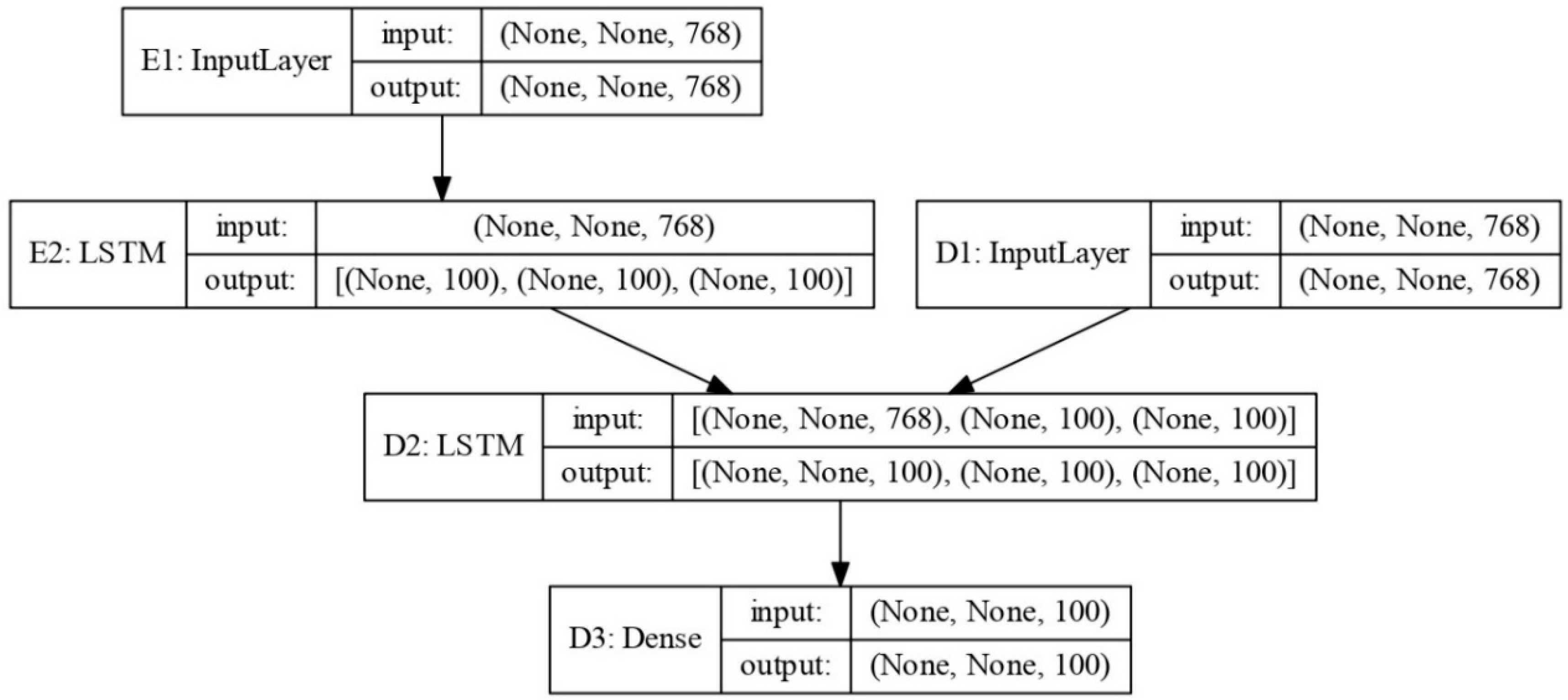
Three different seq2seq architectures (in Figure 2, Figure 3 and Figure 4) explored in our experiments were implemented with the functional API using Tensorflow [30] (the python library used for dataflow and machine learning) with Keras [31] (the python library for deep learning). Used architectures were plotted with the plot_model function in Keras.

All seq2seq architectures were applied on top of word embeddings. In our experiments, we used the following types:

• One-hot encoding. This is a discrete representation of words mapped into corresponding vectors containing all zero values, except for one value equal to 1. Thus, each word is represented by its unique vector with the value of 1 at a different position. A length of such a vector becomes the vocabulary size. Sizes of question and answer vocabularies are not necessary equal; therefore, the lengths of their one-hot encoding vectors are also different.
• FastText (presented in Reference [32]). FastText is a library (offered by Facebook’s AI Research Lab) used to train neural distributional embeddings able to catch semantic similarities between words. In this research, we experiment with English (cc.en.300.vec) and Lithuanian (cc.lt.300.vec) fastText embeddings trained using continuous-bag-of-words (CBOW) with position-weights, in 300 dimensions, with character 5-g of window size five and 10 negatives [33]. Each fastText word embedding is a sum of n-gram vectors incoming into that word (e.g., 5-g chatb, hatbo, atbot n-grams compose the word chatbot). FastText word embeddings can be created even for misspelled words, and the obtained vectors are close to their correct equivalents. This is an advantage for languages having the missing diacritics problem in non-normative texts. Despite the Lithuanian language having this problem, the dataset that we used in this research contained only normative texts.
• BERT (Bidirectional Encoder Representations from Transformers) (offered in Reference [34]). This is Google’s neural-based technique (with multi-directional language modeling and attention mechanisms), which demonstrates state-of-the-art performance on a wide range of NLP tasks, including chatbot technology. Distributional BERT embeddings are also robust to disambiguation problems, i.e., homonyms with BERT are represented by different vectors. In our experiments, we used the BERT service [35] with the base multilingual cased 12-layer, 768-hidden, 12-head model for 104 languages (covering English and Lithuanian).

Different vectorization types were tested in the following encoder–decoder units:

• One-hot encoding with both encoder and decoder;
• FastText (abbreviated ft) embeddings with the encoder and one-hot encoding with the decoder;
• BERT embeddings with the encoder and one-hot encoding with the decoder;
• FastText embeddings with both encoder and decoder;
• BERT embeddings with both encoder and decoder.

5. Experiments and Results

To avoid subjectivity and the high human evaluation cost, the quality of the chatbot output is typically evaluated using machine translation evaluation metrics such as BLUE [36] or text summarization metrics such as ROUGE [37].

The BLEU (Bilingual Evaluation Understudy) score compares the chatbot-generated output text (so-called hypothesis) with a human-produced answer (so-called reference or gold-standard) text and indicates how many n-grams in the output text appear in the reference. The BLUE score can be any value within the interval [0, 1] and is mathematically defined in Equation (2).

$$BLUE=BP\times {\left({\displaystyle \prod }_{n=1}^{N}precisio{n}_n\right)}^{1/N},$$

(2)

where N is the a maximum n-gram number n = [1, N] (N = 4 in our evaluations).

BP (brevity penalty) and ${precision}_n$ are defined with Equations (3) and (4), respectively.

$$BP=\min \left(1,\exp \left(1-\frac{{ref}_{length}}{{out}_{length}}\right)\right),$$

(3)

where ${ref}_{length}$ is a reference length, and $ou{t}_{length}$ is the chatbot output length.

$$precisio{n}_n=\frac{{{\displaystyle \sum }}_n\min \left(m_{out}^n,m_{ref}^n\right)}{{{\displaystyle \sum }}_{n^{\prime }}{m}_{out}^{n^{\prime }}},$$

(4)

where $m_{out}^n$ is the number of n-grams in the chatbot output matching the reference, $m_{ref }^n$ is the number of n-grams in the reference, and ${\displaystyle \sum }_{n^{\prime }}{m}_{out}^{n^{\prime }}$ is the total number of n-grams in the chatbot output.

The BLUE scores were calculated using the python implemented blue_score module from the translate package in the nltk platform [38]. The blue_score parameters were initialized with the default values, except for the smoothing function, which was set to method2 [39] (adding 1 to both numerator and denominator); n-gram weights were set to 0.25 and N = 4.

Depending on the interval the BLUE score values are in, the chatbot result can be interpreted as useless (if BLUE < 10), hard to get the gist (10–19), the gist is clear, but has significant errors (20–29), average quality (30–40), high quality (40–50), very high quality (50–60), and better than human (>60). These values and interpretations were taken from the Google Cloud’s AI and Machine Learning product description in Reference [40].

The ROUGE (Recall-Oriented Understudy for Gisting Evaluation) metric measures the similarity of the chatbot-generated output to the reference text. ROUGE-N_precision, ROUGE-N_recall, and ROUGE-N_f-score are mathematically defined by Equations (5)–(7), respectively.

$$ROUGE{-N}_{precision}=\frac{m_{overlap }^n}{m_{out}^n},$$

(5)

where $m_{out}^n$ is the number of n-grams in the chatbot output, and $m_{overlap}^n$ is the number of overlapping n-grams in the chatbot output and the reference.

$$ROUGE-N_{recall}=\frac{m_{overlap }^n}{m_{ref}^n},$$

(6)

where $m_{ref}^n$ is the number of n-grams in the reference, and $m_{overlap }^n$ is the number of overlapping n-grams in the chatbot output and the reference.

$$ROUGE-N_{f-score}=\frac{2 \times ROUGE-N_{precision}\times ROUGE-N_{recall} }{ROUGE-N_{precision}+ROUGE-N_{recall}}.$$

(7)

In addition to ROUGE-N, we also evaluated ROUGE-L, which measures the longest common subsequence (LCS) of tokens and even catches sentence-level word order. ROUGE-L_precision, ROUGE-L_recall, and ROUGE-L_f-score are mathematically defined by Equations (8)–(10), respectively.

$$ROUGE{-L}_{precision}=\frac{LCS}{m_{out}},$$

(8)

where $m_{out}$ is the number of tokens in the chatbot output.

$$ROUGE{-L}_{recall}=\frac{LCS}{m_{ref}},$$

(9)

where $m_{ref}$ is the number of tokens in the reference.

$$ROUGE{-L}_{f-score}=\frac{2\times ROUGE{-L}_{precision}\times ROUGE{-L}_{recall} }{ROUGE{-L}_{precision}+ROUGE{-L}_{recall}}.$$

(10)

Both ROUGE-N and ROUGE-L differ from the BLUE score because they do not have the brevity penalty (responsible for high-scoring outputs matching the reference text in length). ROUGE-N computes the n-gram match only for the chosen fixed n-gram size n, whereas ROUGE-L searches for the longest overlapping sequence of tokens and does not require defining the n-grams at all. Both ROUGE-N and ROUGE-L can be any value within the interval [0, 1]. Despite this, there are neither defined thresholds nor their interpretations; higher ROUGE-N and ROUGE-L values denote the higher intelligence of the chatbot. Both metrics are important for our intra-comparison purposes.

For ROUGE-N and ROUGE-L evaluation, we used Python library rouge [41], with N = 2 in all our evaluations.

To train and test our seq2seq models and to overcome the problem of a very small dataset (described in Section 3), we used five-fold cross validation (20% of the training data were used for validation). The obtained results were averaged and the confidence intervals (with a confidence level of 95% and alpha = 0.05) were calculated.

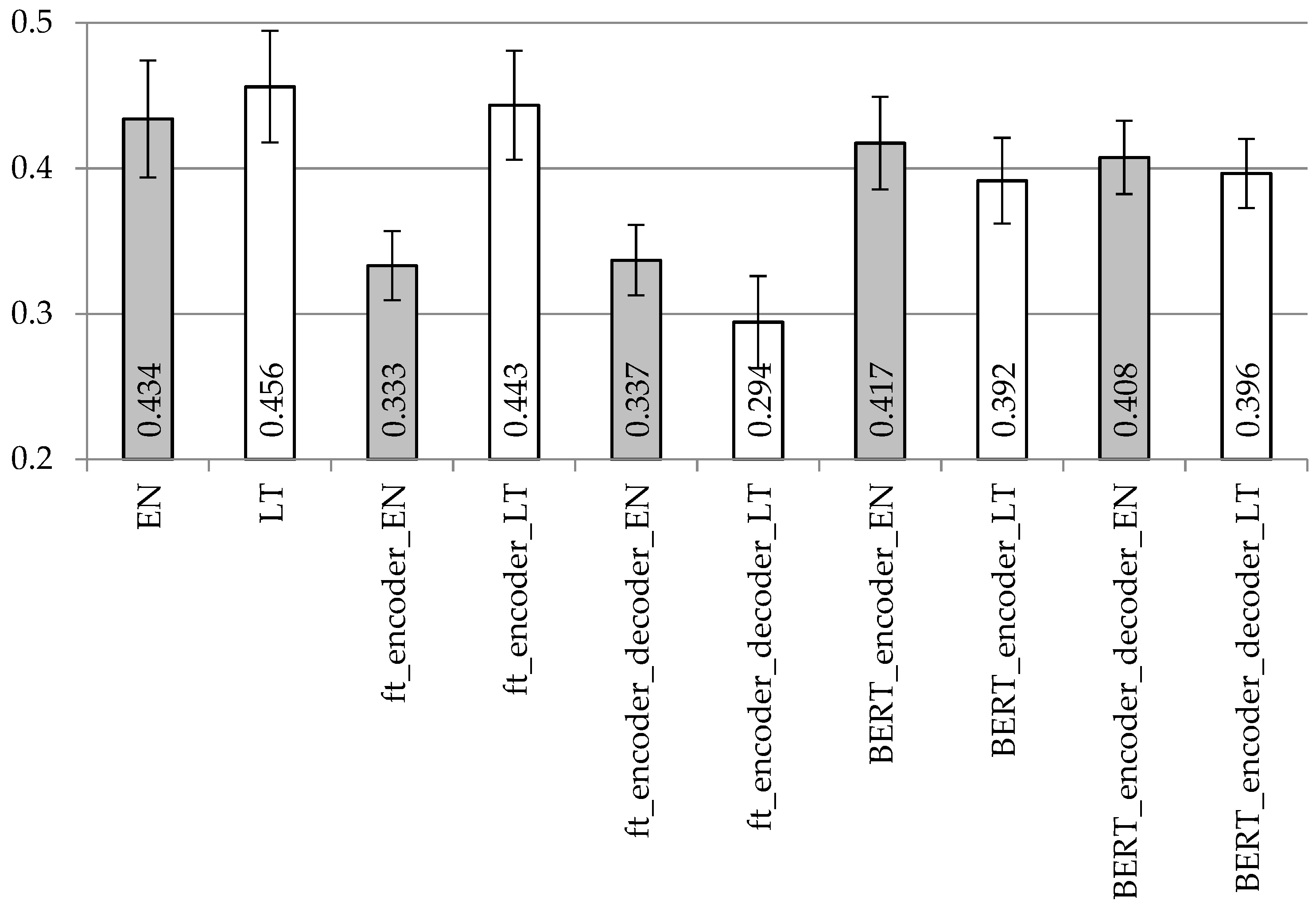
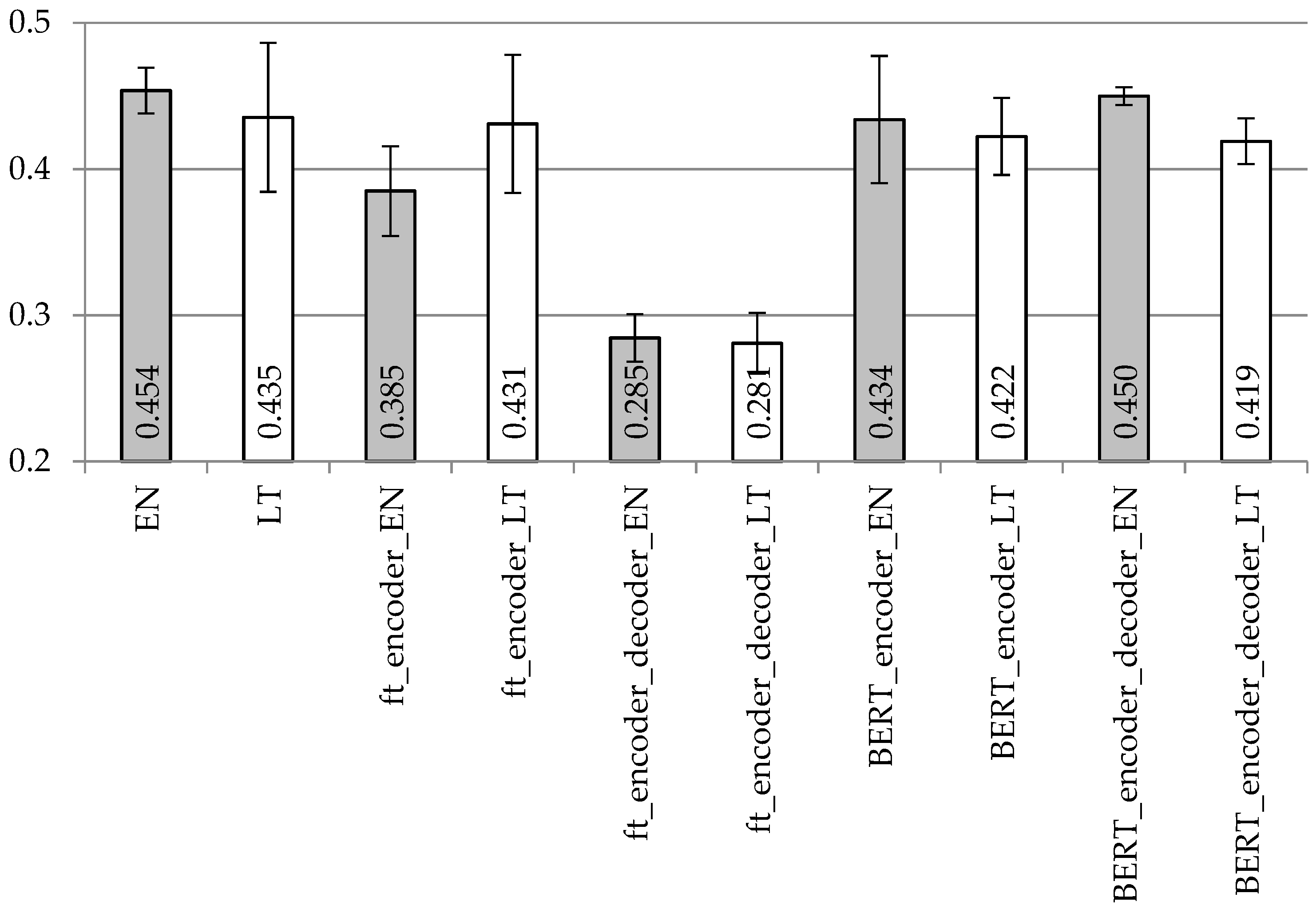
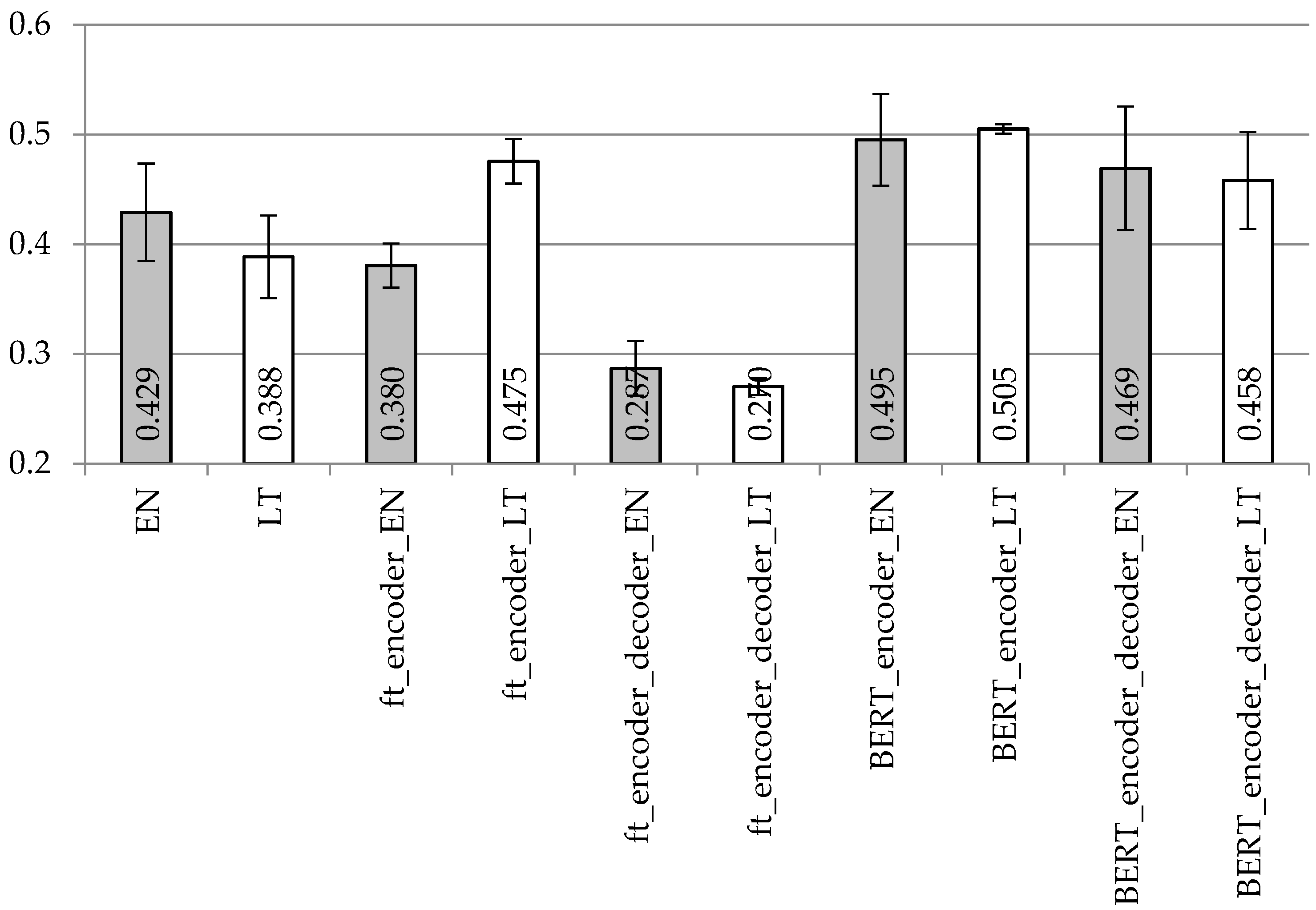
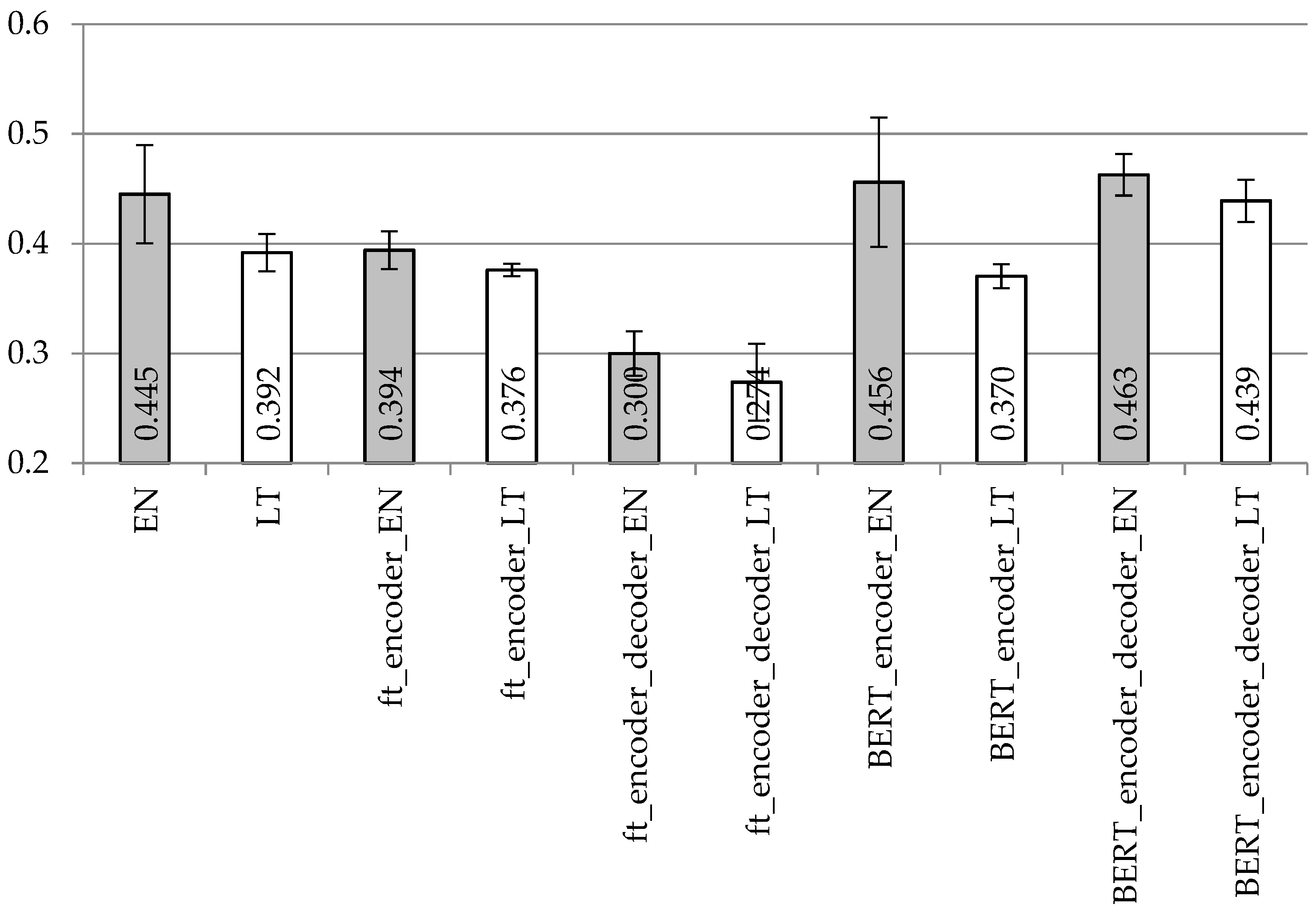
The BLUE scores with the LSTM encoder and decoder model applied using different vectorization types to the datasets with removed and separated punctuation are presented in Figure 5 and Figure 6, respectively. The ROUGE-2 and ROUGE-L precision/recall/f-score values are presented in

Table 2. Averaged Recall-Oriented Understudy for Gisting Evaluation (ROUGE)-2 and ROUGE-L precision/recall/f-score values with confidence intervals using the LSTM encoder and decoder model with different vectorization types on the dataset with removed punctuation. The best values in the column for EN and LT are in bold. BERT—Bidirectional Encoder Representations from Transformers; ft—FastText.

Experiments	ROUGE-2			ROUGE-L
	Precision	Recall	f-Score	Precision	Recall	f-Score
EN	0.458 ± 0.035	0.478 ± 0.025	0.463 ± 0.031	0.525 ± 0.033	0.559 ± 0.022	0.522 ± 0.030
LT	0.467 ± 0.042	0.475 ± 0.044	0.469 ± 0.043	0.526 ± 0.035	0.552 ± 0.045	0.522 ± 0.038
ft_encoder_EN	0.307 ± 0.020	0.323 ± 0.025	0.310 ± 0.022	0.385 ± 0.018	0.423 ± 0.021	0.382 ± 0.017
ft_encoder_LT	0.401 ± 0.038	0.411 ± 0.038	0.403 ± 0.038	0.476 ± 0.039	0.498 ± 0.041	0.470 ± 0.041
ft_encoder_decoder_EN	0.326 ± 0.022	0.363 ± 0.024	0.337 ± 0.023	0.416 ± 0.023	0.483 ± 0.025	0.422 ± 0.024
ft_encoder_decoder_LT	0.296 ± 0.040	0.405 ± 0.060	0.331 ± 0.044	0.372 ± 0.033	0.491 ± 0.050	0.388 ± 0.036
BERT_encoder_EN	0.395 ± 0.034	0.418 ± 0.032	0.401 ± 0.034	0.474 ± 0.029	0.515 ± 0.026	0.474 ± 0.029
BERT_encoder_LT	0.400 ± 0.026	0.427 ± 0.030	0.407 ± 0.027	0.469 ± 0.032	0.518 ± 0.037	0.471 ± 0.034
BERT_encoder_decoder_EN	0.402 ± 0.019	0.426 ± 0.020	0.409 ± 0.019	0.473 ± 0.023	0.517 ± 0.023	0.477 ± 0.023
BERT_encoder_decoder_LT	0.369 ± 0.026	0.386 ± 0.029	0.372 ± 0.026	0.442 ± 0.030	0.472 ± 0.026	0.436 ± 0.025

and

Table 3. Averaged ROUGE-2 and ROUGE-L precision/recall/f-score values with confidence intervals using the LSTM encoder and decoder model with different vectorization types on the dataset with separated punctuation. The best values in the column for EN and LT are in bold.

Experiments	ROUGE-2			ROUGE-L
	Precision	Recall	f-Score	Precision	Recall	f-Score
EN	0.456 ± 0.020	0.474 ± 0.015	0.459 ± 0.016	0.526 ± 0.011	0.558 ± 0.008	0.520 ± 0.007
LT	0.431 ± 0.043	0.431 ± 0.044	0.428 ± 0.043	0.497 ± 0.040	0.515 ± 0.040	0.488 ± 0.041
ft_encoder_EN	0.346 ± 0.028	0.363 ± 0.025	0.349 ± 0.026	0.429 ± 0.024	0.464 ± 0.021	0.425 ± 0.022
ft_encoder_LT	0.380 ± 0.043	0.389 ± 0.045	0.381 ± 0.044	0.454 ± 0.039	0.482 ± 0.037	0.451 ± 0.038
ft_encoder_decoder_EN	0.290 ± 0.018	0.362 ± 0.049	0.312 ± 0.027	0.388 ± 0.023	0.479 ± 0.049	0.397 ± 0.030
ft_encoder_decoder_LT	0.287 ± 0.018	0.411 ± 0.029	0.328 ± 0.022	0.374 ± 0.026	0.508 ± 0.027	0.393 ± 0.026
BERT_encoder_EN	0.428 ± 0.012	0.426 ± 0.007	0.421 ± 0.009	0.511 ± 0.020	0.525 ± 0.011	0.494 ± 0.013
BERT_encoder_LT	0.401 ± 0.028	0.417 ± 0.026	0.404 ± 0.028	0.464 ± 0.022	0.503 ± 0.020	0.460 ± 0.022
BERT_encoder_decoder_EN	0.455 ± 0.012	0.454 ± 0.020	0.448 ± 0.016	0.531 ± 0.007	0.546 ± 0.015	0.513 ± 0.012
BERT_encoder_decoder_LT	0.409 ± 0.027	0.423 ± 0.028	0.410 ± 0.028	0.473 ± 0.021	0.513 ± 0.024	0.471 ± 0.023

, respectively.

Despite the used punctuation treatment, the highest BLUE values (as presented in Figure 5 and Figure 6) with the simple LSTM encoder architecture were achieved using one-hot encoding vectorization for both encoder and decoder. FastText vectorization is recommended only for the encoder and only for the Lithuanian language. Differences in BLUE scores are not so huge with the BERT vectorization, whether for different languages or for different vectorization units (BERT for encoder; BERT for encoder plus decoder).

In Table 2 and Table 3, we see the same trend as in Figure 5 and Figure 6, respectively. Hence, one-hot encoding vectorization for both units is the best solution with the simple LSTM encoder–decoder architecture for both English and Lithuanian languages. FastText vectorization with the encoder and decoder units is not recommended.

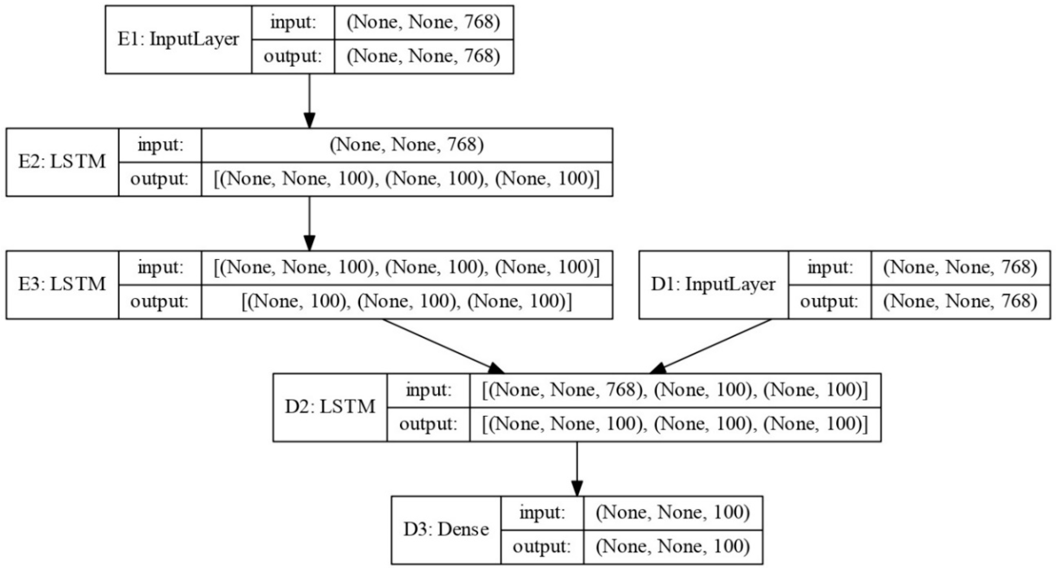
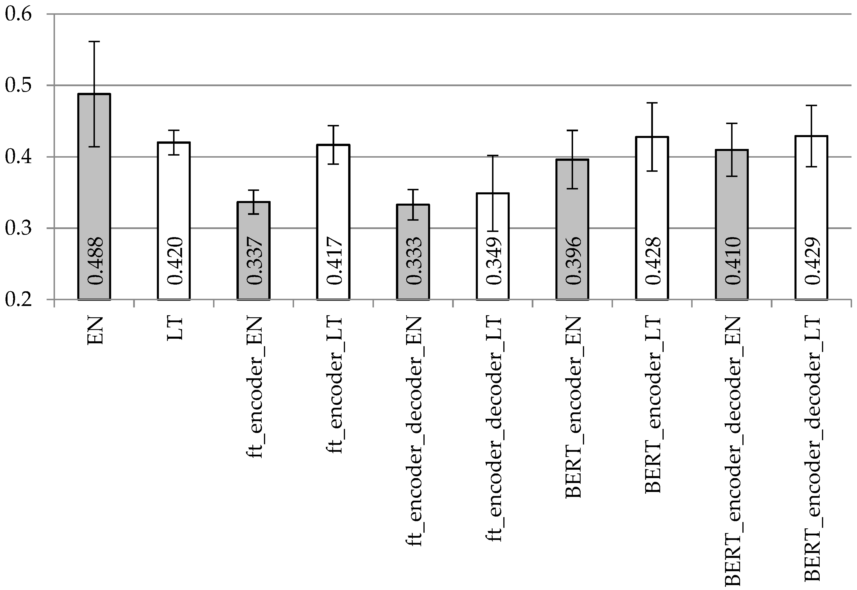
The BLUE scores with the LSTM2 encoder and decoder model applied with different vectorization types to the datasets with removed and separated punctuation are presented in Figure 7 and Figure 8, respectively. The ROUGE-2 and ROUGE-L precision/recall/f-score values are presented in

Table 4. Averaged ROUGE-2 and ROUGE-L precision/recall/f-score values with confidence intervals using the LSTM2 encoder and LSTM decoder model with different vectorization types on the dataset with removed punctuation. The best values in the column for EN and LT are in bold.

Experiments	ROUGE-2			ROUGE-L
	Precision	Recall	f-Score	Precision	Recall	f-Score
EN	0.420 ± 0.033	0.432 ± 0.024	0.416 ± 0.029	0.482 ± 0.032	0.508 ± 0.022	0.469 ± 0.029
LT	0.368 ± 0.031	0.378 ± 0.025	0.368 ± 0.027	0.432 ± 0.025	0.455 ± 0.022	0.423 ± 0.024
ft_encoder_EN	0.331 ± 0.030	0.348 ± 0.045	0.332 ± 0.037	0.416 ± 0.023	0.451 ± 0.047	0.410 ± 0.032
ft_encoder_LT	0.395 ± 0.010	0.405 ± 0.010	0.397 ± 0.011	0.470 ± 0.007	0.490 ± 0.002	0.463 ± 0.006
ft_encoder_decoder_EN	0.298 ± 0.025	0.384 ± 0.030	0.328 ± 0.026	0.404 ± 0.033	0.506 ± 0.027	0.418 ± 0.030
ft_encoder_decoder_LT	0.290 ± 0.030	0.365 ± 0.041	0.315 ± 0.033	0.368 ± 0.027	0.456 ± 0.030	0.379 ± 0.027
BERT_encoder_EN	0.488 ± 0.020	0.488 ± 0.030	0.483 ± 0.026	0.573 ± 0.015	0.585 ± 0.033	0.557 ± 0.026
BERT_encoder_LT	0.469 ± 0.021	0.476 ± 0.018	0.470 ± 0.020	0.528 ± 0.018	0.553 ± 0.019	0.525 ± 0.017
BERT_encoder_decoder_EN	0.446 ± 0.048	0.441 ± 0.047	0.438 ± 0.046	0.531 ± 0.036	0.536 ± 0.030	0.510 ± 0.032
BERT_encoder_decoder_LT	0.421 ± 0.042	0.435 ± 0.032	0.423 ± 0.039	0.481 ± 0.040	0.518 ± 0.028	0.481 ± 0.039

and

Table 5. Averaged ROUGE-2 and ROUGE-L precision/recall/f-score values with confidence intervals using the LSTM2 encoder and LSTM decoder model with different vectorization types on the dataset with separated punctuation. The best values in the column for EN and LT are in bold.

Experiments	ROUGE-2			ROUGE-L
	Precision	Recall	f-Score	Precision	Recall	f-Score
EN	0.445 ± 0.044	0.458 ± 0.046	0.446 ± 0.042	0.503 ± 0.031	0.530 ± 0.025	0.497 ± 0.026
LT	0.415 ± 0.051	0.429 ± 0.052	0.417 ± 0.052	0.475 ± 0.043	0.498 ± 0.049	0.464 ± 0.047
ft_encoder_EN	0.320 ± 0.024	0.337 ± 0.028	0.323 ± 0.025	0.408 ± 0.020	0.445 ± 0.029	0.406 ± 0.020
ft_encoder_LT	0.369 ± 0.038	0.380 ± 0.040	0.371 ± 0.039	0.442 ± 0.031	0.460 ± 0.033	0.435 ± 0.026
ft_encoder_decoder_EN	0.347 ± 0.021	0.399 ± 0.023	0.365 ± 0.021	0.449 ± 0.023	0.505 ± 0.031	0.448 ± 0.022
ft_encoder_decoder_LT	0.339 ± 0.039	0.421 ± 0.039	0.368 ± 0.037	0.421 ± 0.033	0.502 ± 0.028	0.433 ± 0.030
BERT_encoder_EN	0.396 ± 0.045	0.417 ± 0.048	0.400 ± 0.048	0.477 ± 0.036	0.519 ± 0.040	0.473 ± 0.039
BERT_encoder_LT	0.418 ± 0.051	0.444 ± 0.050	0.424 ± 0.050	0.479 ± 0.045	0.520 ± 0.039	0.475 ± 0.042
BERT_encoder_decoder_EN	0.407 ± 0.042	0.431 ± 0.045	0.413 ± 0.043	0.484 ± 0.033	0.533 ± 0.040	0.484 ± 0.037
BERT_encoder_decoder_LT	0.392 ± 0.037	0.417 ± 0.036	0.399 ± 0.037	0.452 ± 0.040	0.496 ± 0.030	0.455 ± 0.039

, respectively.

When comparing Figure 7 with Figure 8 representing the BLUE scores with the stacked LSTM encoder, it is difficult to draw very firm conclusions. One-hot encoding for both encoder and decoder units remains the best vectorization technique on the English dataset with the separated punctuation. However, if excluding this particular result, BERT vectorization (for the encoder or encoder plus decoder) stands out with the best achieved BLUE values for both languages. Surprisingly, with the separated punctuation and BLUE vectorization, the results on the Lithuanian dataset are even better. When comparing Figure 5 with Figure 7 (simple LSTM with stacked LSTM on the removed punctuation) and Figure 6 with Figure 8 (simple LSTM with stacked LSTM on the separated punctuation), the stacked LSTM encoder demonstrates similar results with the fastText encoding; however, BERT encoding is recommended with the removed punctuation for both languages, but it is definitely not the choice with separated punctuation in the English language.

Table 4 and Table 5 demonstrate a similar trend to Figure 7 and Figure 8, respectively.

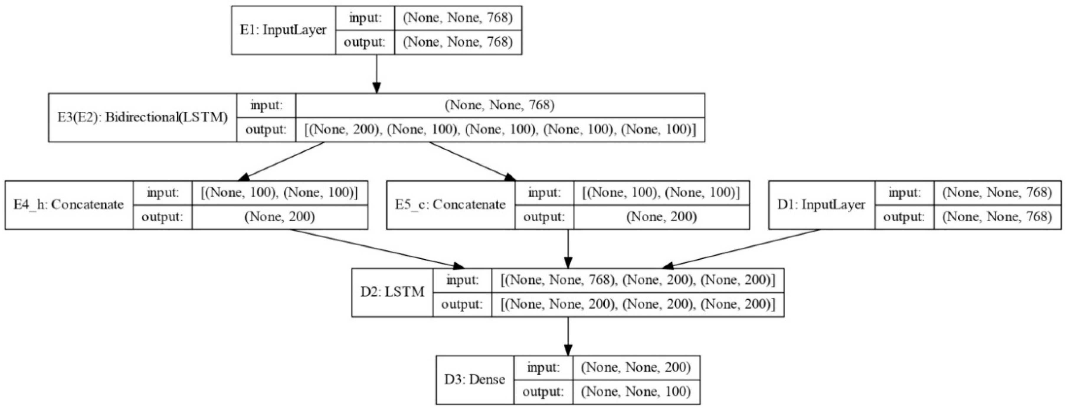
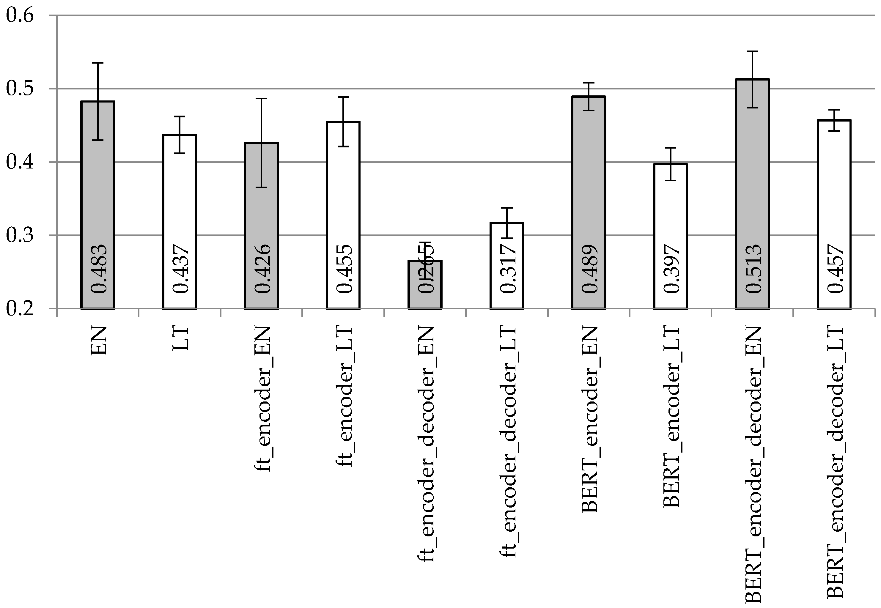
The BLUE scores with the BiLSTM encoder and decoder model applied with different vectorization types to the datasets with removed and separated punctuation are presented in Figure 9 and Figure 10, respectively. The ROUGE-2 and ROUGE-L precision/recall/f-score values are presented in

Table 6. Averaged ROUGE-2 and ROUGE-L precision/recall/f-score values with confidence intervals using the BiLSTM encoder and LSTM decoder model with different vectorization types on the dataset with removed punctuation. The best values in the column for EN and LT are in bold.

Experiments	ROUGE-2			ROUGE-L
	Precision	Recall	f-Score	Precision	Recall	f-Score
EN	0.442 ± 0.018	0.455 ± 0.024	0.445 ± 0.020	0.512 ± 0.014	0.545 ± 0.019	0.510 ± 0.014
LT	0.413 ± 0.058	0.415 ± 0.057	0.411 ± 0.056	0.477 ± 0.059	0.488 ± 0.058	0.466 ± 0.055
ft_encoder_EN	0.368 ± 0.045	0.387 ± 0.043	0.373 ± 0.045	0.462 ± 0.043	0.492 ± 0.033	0.456 ± 0.039
ft_encoder_LT	0.414 ± 0.027	0.419 ± 0.021	0.413 ± 0.025	0.472 ± 0.026	0.491 ± 0.015	0.464 ± 0.026
ft_encoder_decoder_EN	0.290 ± 0.038	0.407 ± 0.043	0.328 ± 0.040	0.391 ± 0.039	0.508 ± 0.028	0.406 ± 0.037
ft_encoder_decoder_LT	0.325 ± 0.007	0.479 ± 0.016	0.372 ± 0.011	0.398 ± 0.007	0.563 ± 0.016	0.421 ± 0.009
BERT_encoder_EN	0.468 ± 0.015	0.477 ± 0.025	0.467 ± 0.018	0.561 ± 0.006	0.576 ± 0.018	0.546 ± 0.009
BERT_encoder_LT	0.392 ± 0.031	0.415 ± 0.027	0.398 ± 0.031	0.465 ± 0.031	0.520 ± 0.021	0.465 ± 0.032
BERT_encoder_decoder_EN	0.496 ± 0.020	0.504 ± 0.016	0.495 ± 0.018	0.571 ± 0.018	0.601 ± 0.007	0.565 ± 0.014
BERT_encoder_decoder_LT	0.428 ± 0.024	0.445 ± 0.024	0.431 ± 0.023	0.483 ± 0.021	0.525 ± 0.031	0.482 ± 0.023

and

Table 7. Averaged ROUGE-2 and ROUGE-L precision/recall/f-score values with confidence intervals using the BiLSTM encoder and LSTM decoder model with different vectorization types on the dataset with separated punctuation. The best values in the column for EN and LT are in bold.

Experiments	ROUGE-2			ROUGE-L
	Precision	Recall	f-Score	Precision	Recall	f-Score
EN	0.420 ± 0.033	0.432 ± 0.024	0.416 ± 0.029	0.482 ± 0.032	0.508 ± 0.022	0.469 ± 0.029
LT	0.368 ± 0.031	0.378 ± 0.025	0.368 ± 0.027	0.432 ± 0.025	0.455 ± 0.022	0.423 ± 0.024
ft_encoder_EN	0.331 ± 0.030	0.348 ± 0.045	0.332 ± 0.037	0.416 ± 0.023	0.451 ± 0.047	0.410 ± 0.032
ft_encoder_LT	0.395 ± 0.010	0.405 ± 0.010	0.397 ± 0.011	0.470 ± 0.007	0.490 ± 0.002	0.463 ± 0.006
ft_encoder_decoder_EN	0.298 ± 0.025	0.384 ± 0.030	0.328 ± 0.026	0.404 ± 0.033	0.506 ± 0.027	0.418 ± 0.030
ft_encoder_decoder_LT	0.290 ± 0.030	0.365 ± 0.041	0.315 ± 0.033	0.368 ± 0.027	0.456 ± 0.030	0.379 ± 0.027
BERT_encoder_EN	0.446 ± 0.048	0.441 ± 0.047	0.438 ± 0.046	0.531 ± 0.036	0.536 ± 0.030	0.510 ± 0.032
BERT_encoder_LT	0.421 ± 0.042	0.435 ± 0.032	0.423 ± 0.039	0.481 ± 0.040	0.518 ± 0.028	0.481 ± 0.039
BERT_encoder_decoder_EN	0.488 ± 0.020	0.488 ± 0.030	0.483 ± 0.026	0.573 ± 0.015	0.585 ± 0.033	0.557 ± 0.026
BERT_encoder_decoder_LT	0.469 ± 0.021	0.476 ± 0.018	0.470 ± 0.020	0.528 ± 0.018	0.553 ± 0.019	0.525 ± 0.017

, respectively.

With the BiLSTM encoder, BLUE values in Figure 9 and Figure 10 are the highest with the BERT vectorization in both languages, especially when BERT vectorization is used for both encoder and decoder units. However, fastText vectorization for both encoder and decoder is not recommended for any of the used languages. When comparing BiLSTM encoder values with the appropriate simple LSTM or stacked LSTM values in Figure 5, Figure 6, Figure 7 and Figure 8, the recommendation would be to use more sophisticated architectures. If choosing the appropriate vectorization, stacked LSTM works better using the English dataset and BiLSTM works better using the Lithuanian dataset.

As presented in Table 6 and Table 7, BERT vectorization is the best choice with the BiLSTM encoder. The conclusions from ROUGE-2 and ROUGE-L values in Table 6 and Table 7 are consistent with the conclusions drawn from the appropriate BLUE values in Figure 9 and Figure 10, respectively.

6. Discussion

Focusing on the results (when BLUE is considered as the primary metric and ROUGE is considered as the auxiliary metric for our analysis) allows us to make the statements below. Although with some small exceptions, there is a correlation between calculated BLUE scores and ROUGE-2/ROUGE-L values.

In most of the cases, results on datasets with separated punctuation were a bit lower compared to results with the removed punctuation pre-processing. This is because the separated punctuation task is more complicated; instead of generating words only, the seq2seq model has to generate both words and punctuation. The detailed error analysis revealed that the majority of errors were due to the incorrectly generated punctuation marks. Despite the language and the punctuation pre-processing type, the worst BLUE score values were calculated with the fastText embedding vectorization for both encoder and decoder units (ft_encoder_decoder). Furthermore, results on the Lithuanian dataset were even worse compared to English. On the contrary, the performance of the fastText encoder with one-hot decoding on the Lithuanian dataset was obviously better compared to English in all cases except for the dataset with separated punctuation and BiLSTM encoder and LSTM decoder.

However, BERT embeddings are definitely the better choice compared to fastText. With the LSTM encoder and decoder and the BiLSTM encoder and LSTM decoder models, BERT performed better in English, whereas the stacked LSTM encoder architecture (i.e., with the LSTM2 encoder and LSTM decoder) applied to BERT embeddings was more suitable for the morphologically complex Lithuanian.

One-hot vectorization for both encoder and decoder units with the simple LSTM encoder and decoder model outperformed other vectorization types. With more complex encoder units (i.e., stacked LSTM or BiLSTM), one-hot encoding was the best choice only for the separated punctuation dataset for the English language; however, in all other cases, it was outperformed by BERT embeddings.

The overall best BLUE/ROUGE-2_f-score/ROUGE-L_f-score values on the English dataset with removed punctuation pre-processing were ~0.513/~0.495/~0.565. These results were achieved with the BiLSTM encoder and LSTM decoder model applied with BERT embeddings for both encoder and decoder units. The best BLUE/ROUGE-2_f-score/ROUGE-L_f-score values on the Lithuanian dataset with removed punctuation were a bit lower, i.e., ~0.505/~0.470/~0.525. Values were obtained with the stacked LSTM2 encoder and LSTM decoder with BERT embeddings for the encoder unit and one-hot vectorization for the decoder. The best BLUE value (~0.488) on the English dataset with separated punctuation was calculated using the stacked LSTM2 encoder and LSTM decoder model applied on top of one-hot vectorization for both units. The best ROUGE-2_f-score and ROUGE-L_f-score values equal to ~0.483 and ~0.557, respectively, were achieved with the BiLSTM encoder and LSTM decoder model and BERT embeddings for both units. The best BLUE/ROUGE-2_f-score/ROUGE-L_f-score values equal to ~0.439/~0.470/~0.525 on the Lithuanian dataset with separated punctuation were achieved using the BiLSTM encoder and LSTM decoder model and BERT embeddings for both units.

The lowest calculated BLUE score values (as a percentage) for both English and Lithuanian fell into the range 20–29, which means that the gist of the generated answers was still clear, but had significant errors (as explained in Section 5). The highest achieved values on the dataset with removed punctuation were at the beginning of the interval 50–60; therefore, the quality of the generated answers was considered as very high; the highest values in the dataset with separated punctuation was in the range 40–50 that is still considered as high quality. This allows us to conclude that the results are accurate enough to be applied in practice.

Despite practical benefits, this work also brings a scientific contribution. Generative chatbots were never previously trained for a morphologically complex language (such as Lithuanian). Furthermore, in general, they were never trained on such a small dataset. In addition to testing different encoder–decoder architectures (simple LSTM encoder, stacked LSTM encoder, BiLSTM encoder), different embedding types (one-hot, fastText, BERT), and different vectorization options (only encoder, encoder plus decoder), we tested two very different languages and formulated recommendations regarding what works best for each of these languages. Moreover, we anticipate that, for languages with similar characteristics under similar experimental conditions, similar results can be expected.

In addition to positive things, limitations of the investigated approach need to be mentioned as well. Similar accuracy can be expected only if the used dataset is in a closed domain and contains a limited number of topics. In our case, we tested the dataset covering rephrased questions and answers about a company’s products, as well as their prices, used technologies, and supported languages. Thus, such a generative chatbot cannot answer questions that are unrelated. Furthermore, BERT embeddings are recommended as the best vectorization option; however, these embeddings are supported for a limited number of languages (i.e., ~100 languages).

7. Conclusions

In this research, we presented the first generative chatbot results obtained on very small domain-specific datasets for English and morphologically complex Lithuanian languages.

We investigated different encoder–decoder architectures (with LSTM, stacked LSTM, and BiLSTM), different embedding types (one-hot, fastText, and BERT), different vectorization types in different encoder and decoder units, and different punctuation treatment (its removal or separation).

The best BLUE values on the English/Lithuanian datasets with removed and separated punctuation were ~0.513/~0.505 and ~0.488/~0.439, respectively. This research revealed that more complex architectures (based on the stacked LSTM and BiLSTM encoders) are more accurate compared to simple LSTM. It also demonstrates the advantages of BERT embeddings. Despite BLUE values for the Lithuanian language being a bit lower, compared to English, the results are good enough to be applied in practice. This research is important and interesting because (1) generative chatbots are trained on very small domain-specific data, and (2) it reports the first generative chatbot results for a morphologically complex language.

Despite the search for effective solutions on small datasets being much more challenging, in future research, we are planning to augment our datasets with newly covered topics, to experiment with different seq2seq architectures by tuning their hyper-parameters.