A Causality Mining and Knowledge Graph Based Method of Root Cause Diagnosis for Performance Anomaly in Cloud Applications

Abstract

With the development of cloud computing technology, the microservice architecture (MSA) has become a prevailing application architecture in cloud-native applications. Many user-oriented services are supported by many microservices, and the dependencies between services are more complicated than those of a traditional monolithic architecture application. In such a situation, if an anomalous change happens in the performance metric of a microservice, it will cause other related services to be downgraded or even to fail, which would probably cause large losses to dependent businesses. Therefore, in the operation and maintenance job of cloud applications, it is critical to mine the causality of the problem and find its root cause as soon as possible. In this paper, we propose an approach for mining causality and diagnosing the root cause that uses knowledge graph technology and a causal search algorithm. We verified the proposed method on a classic cloud-native application and found that the method is effective. After applying our method on most of the services of a cloud-native application, both precision and recall were over 80%.

1. Introduction

With the emergence of enterprise digital transformation, it has become practical for enterprise applications to migrate to a cloud platform. As cloud computing technology has developed, microservice architecture (MSA) has become a prevailing web application architecture. MSA divides complex software systems into single-function service components and can be independently developed and deployed. MSA is similar to the earlier service-oriented architecture (SOA). It further refines the concept of servicing but does not emphasize the heavy-duty service bus in the SOA framework. However, due to the numerous components of microservices, the complex dependencies between services and the frequent updates of system versions based on microservices inevitably increase the probability of failure and the difficulty of problem diagnosis. Particularly when one of the components is abnormal or has failed, the effect of the anomaly or failure continues to spread with the calls between the components, eventually leading to an overall application quality decline. Therefore, in the operation and maintenance (O&M) task in MSA applications, it is important to find the root cause as soon as possible.

MSA is not a miracle cure; it has problems in many of its aspects. Here are some of the O&M related challenges:

• Large number of services and high expense. In a monolithic architecture, only one application must be guaranteed to run normally, whereas, in microservices, dozens or even hundreds of services need to be guaranteed to run and cooperate normally, which is a great challenge to O&M.
• Complex hosting environment. The hierarchy of the hosting environment for services is complex, and the corresponding network architecture is even more complex. Managing microservices depends on a container environment, which usually runs on a container management platform such as Kubernetes. The container environment is deployed on a virtual machine, which depends on a complex cloud infrastructure environment. The call dependencies among entities at the same level and among entities across levels are of high complexity.
• Large number of monitoring metrics. Based on the two facts above, application performance management (APM) and monitoring must monitor the metrics at least at the service, container, server, and system levels, especially when the properties of each indicator are different.
• Rapid iteration. Microservices can be deployed in many different ways. The development of microservices now follows the principles of DevOps, one of which requires versioning and continuous iterative updating. Obviously, continuous iterative updating poses great difficulty for the timeliness of O&M.

In conclusion, traditional anomaly diagnosis methods are usually based on key performance indicator (KPI) thresholds. System administrators set the KPI monitoring threshold manually according to their domain knowledge for early warning. However, due to the very large number of services in the MSA application and the complex dependencies between services, it is difficult for system administrators to detect anomalies by setting reasonable KPI monitoring thresholds, let alone diagnose root causes in fine granularity. Currently, most studies of root cause analysis (RCA) rely mainly on monitoring data, including log data, service dependency data, and path tracking data. We used knowledge graph technology and a causal search algorithm to help solve the RCA problem. In brief, our contributions can be summarized as follows:

• The proposed system is the first RCA approach for cloud-native applications to combine a knowledge graph and a causality search algorithm.
• We have implemented a prototype for generating a causality graph and sorting possible root causes.
• We have proved experimentally that the proposed approach can rank the root causes in the top two with over 80% precision and recall for most scenarios.

The rest of this paper is structured as follows: Related work is discussed in Section 2. The problem and the proposed solution are described in Section 3. An empirical study is demonstrated in Section 4, and Section 5 summarizes the conclusions and describes planned work.

2. Related Work

Many research papers on RCA focus on complex large-scale systems [1,2,3,4]; they can be grouped into the following categories:

Event correlation analysis-based methods. These methods correlate activity events to identify the root cause of an anomaly or failure. Marvasti et al. [5] introduced a new model of statistical inference to manage complex IT infrastructures based on their anomaly events data obtained from an intelligent monitoring engine. Zeng et al. [6] proposed a parametric model to describe noisy time lags from fluctuating events.

Log-based methods. The common approach to RCA is to analyze log files to identify problems that occurred in the system. The problems are then examined to identify potential causes. The authors in [7,8] introduced a classic log mining method to diagnose and locate anomalies in traditional distributed systems. According to the research in [9,10,11], the log mining method also plays an important role in the RCA of cloud applications. However, not all abnormal behaviors are recorded in logs: in many cases of RCA, in addition to log mining, O&M personnel have to combine their domain experience to find the root cause.

Execution path mining-based methods. The execution path mining-based method is usually suitable for online RCA. It often traces transaction flows between services or components and provides a clear view to identify problem areas and potential bottlenecks. There is already much research on this and many popular tools, such as ptrace [12], Pinpoint [13], AutoPath [14], and CloRExPa [15]. This path mining kind of method can usually solve some intuitive problems, but, for problems requiring inferring causality, the execution path mining-based method usually does not work well.

Dependency graph mining-based methods. In recent years, more and more studies have been based on dependency graphs. In the RCA research for cloud applications, the most representative are related studies from Chen et al. [16,17,18,19], Nie et al. [20], Lin et al. [21], and Asai et al. [22]. These methods are usually used to find the root cause of the problem at the component and service levels to establish a dependency or causality graph and a cause and effect graph based on performance indicators. Most of those authors claimed that the methods they proposed can completely solve the problem of RCA without expert knowledge.

We have found no relevant work on combining a knowledge graph and a causal search algorithm to find the root cause of a defect or failure in a cloud platform.

Inspired by the paper from Lisa et al. [23], it is not difficult to draw a conclusion that automated root cause analysis reduces the overall dependency on expert knowledge, but it doesn’t diminish the value of on-site experts who are vital in monitoring, validating, and managing the RCA process. Therefore, the proposed method is based on a dependency graph-based method, but we introduce knowledge graph technology, which is a kind of knowledge database. As a result, the proposed method is more scalable.

3. Problem Description and Proposed Solution

In this section, we will try to formally define the problem that our method is to solve. Then, we will elaborate the methodological framework of the proposed method in detail.

3.1. Problem of Finding a Root Cause

The O&M entity is defined as subject: let $(S_1,S_2,..S_n)$ denote n subjects, and APM monitor all the subjects S by collecting the performance metrics corresponding to the subject $S_i$. $(M_i,S_j)$ means that metric $M_i$ locates on subject $S_j$, and some key performance metrics are also commonly called $KPI$.

The observation data of a KPI M are a kind of time-series sequence data, which can be denoted as $KP{I}_{data}=\{m_{t_1},m_{t_2},\dots ,m_{t_n}\}$, where $m_{t_i}$ is the observation value for the KPI at the timestamp $t_i$.

Let $Y_{t_i}$ be the variable indicating whether an anomaly happened at the moment $t_i$, $Y_{t_1}$ is 0 or 1.

Let us define an $n\times t$ matrix M, where ${\left[M\right]}_{i,j}=m_{i,j},(i\in [0,n],j\in [0,t])$ is the metric value of subject $S_i$ at timestamp j, and the total number of the given observable subjects is n. Because there is more than one metric for monitoring, all the metrics observation data could be denoted by $M_N=\{{\left[M_1\right]}_{i,j},{\left[M_2\right]}_{i,j},\dots ,{\left[M_n\right]}_{i,j}\}$.

On the basis of the above definition, the root cause finding problem is formulated as follows: Given $M_N$, assuming an anomaly is observed from metric $M_i$ at a certain timestamp $t_i$, that is, $Y_{t_i}=1$, our goal is to find a set of subjects $S_{rc}$ and their metrics $M_{rc}$ as the root cause of the anomaly.

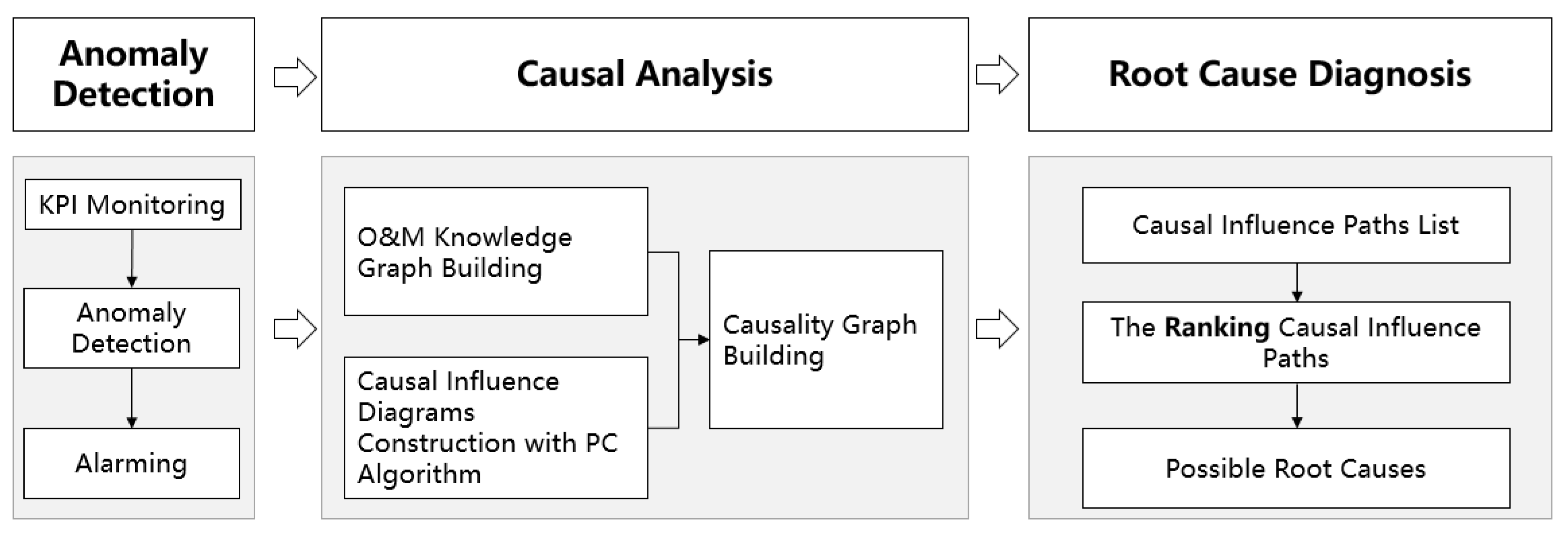
3.2. Method of the Proposed Approach

The workflow of the proposed method is shown in Figure 1. The workflow has three stages: anomaly detection, causal analysis, and root cause diagnosis.

In our previous research [24], we focused on anomaly detection methods. This paper focuses instead on casual analysis and root cause diagnosis. To solve the problem, we introduce a knowledge graph and a causal search algorithm that is based on a PC algorithm [25]. Section 3.2.1 introduces the framework in detail.

3.2.1. O&M Knowledge Graph Construction

This section describes the general construction method of an O&M knowledge graph of a microservice-based system in a cloud environment and explains how to analyze, extract, store, and mine the relevant O&M knowledge.

O&M knowledge includes O&M subjects and their relational attributes, data monitoring, and historical O&M knowledge data. Historical O&M knowledge data are used for restoring the system O&M information at a specific timestamp. By comparatively analysing data at different time points, it is convenient for O&M personnel to see the distribution and change of resources, and, to a certain extent, it plays an important role in anomaly diagnosis and investigation.

A knowledge graph can be represented by a resource description framework (RDF) [26], which is a subject, predicate, and object as shown in Equation (1), and sometimes called a statement:

$$Subject\underrightarrow{predicate}Object$$

(1)

An RDF consists of nodes and edges. Nodes represent entities and attributes, and edges represent the relations between entities and entities and the relations between entities and attributes. RDF data can be stored after serialization. RDF serialization includes RDF/XML, N-Triples, Turtle, RDFa, and JSON-LD. We used RDF/XML in our study.

O&M subjects include software and hardware and their running statuses. Software includes services, microservices, middleware, storage services, databases, and containers. Hardware includes a computer room, a cluster, a server physical rack, a virtual machine, a container, a hard disk, and a router. The characteristics of O&M subjects can be mined from the monitoring data, which commonly include metrics, log events, and tracing data. Figure 2 is a simple sample of a knowledge graph of an MSA system. There is a “calling–called” predicate relation between microservices, a “hosting–hosted” predicate relation between microservices and containers, and a “locating–located” predicate relation between containers and physical servers.

Anomalies are usually observed from some monitoring indicators. For microservices, response and latency times are important key performance indicators (KPIs). We can extract more static attributes or KPIs from other subjects such as memory usage and cache-related KPIs for the physical server and container, and this information could be also represented on the knowledge graph, as shown in Figure 3.

Section 4 describes the construction of the O&M knowledge graph for an MSA application in the Kubernetes environment.

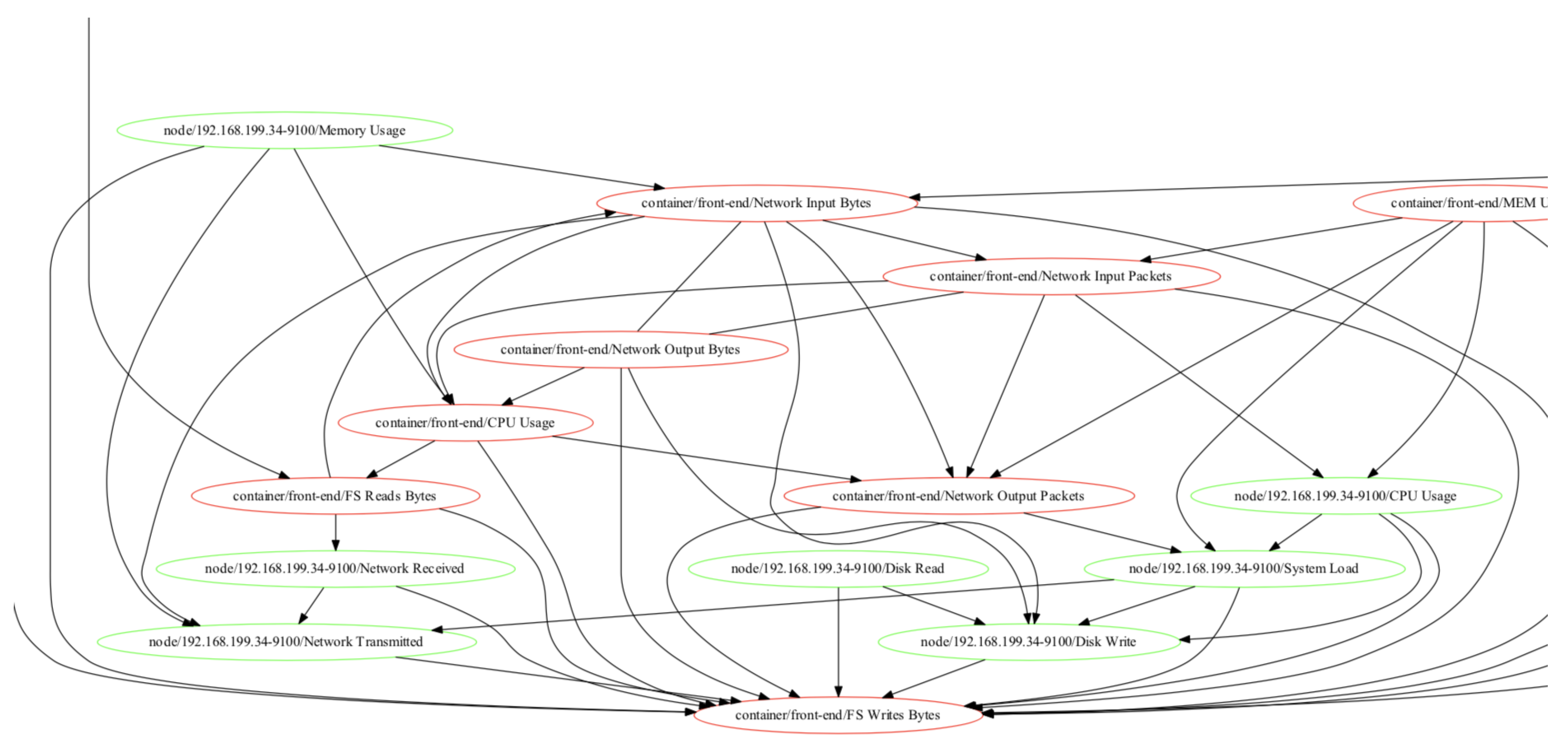
3.2.2. Causality Graph Construction

The causal analysis method proposed in this paper constructs a causality graph with KPI data. The definition of causality is that given two performance indicators X and Y, if performance indicator X affects another performance indicator Y, it is denoted as a directed edge $X\to Y$, or we say X caused Y; in other words, X is a parent of Y. If we can clarify the causality relation between two performance indicators X and Y, but it is not clear whether X affects Y or Y affects X, then it could be denoted by $X-Y$ with undirected edges. Note that, in the causality graph, there is no circuit between two indicators, which means they cause each other. Thus, an ideal causality graph is actually a directed acyclic graph (DAG), as in Definition 1.

Definition 1.

Given a DAG $G=(V,E)$ which is a directed graph without any circle, in which case we call it Bayesian network, where V is a set of vertices, and E is a set of edges, E is connected by vertices. $E\subseteq V\times V$, if G is directed, for each $(i,j)\in V$ could be denoted by $i\to j$. The set of vertices that are adjacent to A in graph G is defined as $adj(A,G)$.

To construct the causality graph in this study, we used the main idea of a PC algorithm, as proposed by Peter Spirtes and Clark Glymour [25]. The main workflow consists of two stages: DAG skeleton construction and direction orientation.

• In the DAG skeleton construction stage, the algorithm first constructs a complete graph with performance indicators as nodes in the dataset. Then, for any two performance indicators X and Y, the algorithm determines whether there is a causal relation between X and Y by judging whether X and Y are conditionally independent as defined in Definition 2. If X and Y conditions are independent, it shows that there is no causal relation between X and Y, and then the corresponding edges are deleted in the complete graph. Finally, a preliminary causal relation graph containing only undirected edges is obtained.
• In the direction orientation stage, the algorithm determines the direction of some edges in the existing causal relation graph according to the d-separation principle defined in Definition 3 and some logic inference rules. The final algorithm will output a causality graph containing directed and undirected edges.

Definition 2.

Suppose X, Y, and Z Subset is defined on probability space $(\Omega ,X,P)$, if $P\left(X\right|Y,Z)=P(X\left|Z\right)$, then X and Y is CI (conditional independent) under Z, denoted by $X\perp Y|Z$.

To judge the conditional independence of continuous data, we adopted the null hypothesis and Fisher z-transformation method. The essence of conditional independence is to judge the independence of X and Y under a given Z. The conventional approach is to do it in two steps:

• The first step is to respectively calculate the regression residuals $r_X$ of X on Z and the regression residuals $r_Y$ of Y on Z. Regression methods (such as the least squares method) are used to calculate the residuals; they can be denoted as $r_X=X-\alpha Z$ and $r_Y=Y-\alpha Z$, where $\alpha$ is the correlation coefficient of the variables X and Y.
• The second step is to calculate the partial correlation coefficient. Calculate the correlation coefficients of the residuals $r_X$ and $r_Y$ and the partial correlation coefficients ${\rho }_{XY·Z}$.

Assume that all variables follow a multidimensional normal distribution, and the partial correlation coefficient ${\rho }_{XY·Z}=0$ if and only if $X\perp Y|Z$.

In this study, we tested whether the null hypothesis ${\rho }_{XY·Z}=0$ is accepted using Fisher’s z:

$$z\left({\widehat{\rho }}_{XY·Z}\right)=\frac{1}{2}ln\left(\frac{1+{\widehat{\rho }}_{XY·Z}}{1-{\widehat{\rho }}_{XY·Z}}\right)$$

(2)

After the above transformation, $\sqrt{n-\left|Z\right|-3}·z\left({\widehat{\rho }}_{XY·Z}\right)$ follows a normal distribution, where $\left|Z\right|$ is the number of performance indicators in Z. Thus, when $\sqrt{n-\left|Z\right|-3}·z\left({\widehat{\rho }}_{XY·Z}\right)>{\mathsf{\Phi }}^{-1}(1-\alpha /2)$, reject the null hypothesis where $\mathsf{\Phi }(·)$ is the cumulative density function of the normal distribution.

Definition 3.

Given a DAG G=(V,E), in which X,Y,Z are disjoint set of variables. X and Y is said to be d-separated by Z, denoted as $X⨿Y|Z$ or $dse{p}_G(X,Z,Y)$, if and only if Z blocks every path from a variable in X to a variable in Y, satisfying either of the following conditions:

• If there exists a  chain$X_i\to Z_m\to Y_j$ where $X_i\in X,Y_j\in Y$, then $Z_m$ must be in $Z.$
• If there exists a radiation$X_i\leftarrow Z_m\to Y_j$ where $X_i\in X,Y_j\in Y$, then $Z_m$ must be in $Z.$
• If there exists a  collider(v-structure) $X_i\to Z_m\leftarrow Y_j$ where $X_i\in X,Y_j\in Y$, then $Z_m$ and the descendants of $Z_m$ MUST NOT be in $Z.$

Because we will optimize the PC algorithm in combination with the knowledge graph technology mentioned above, the pseudocode of this algorithm is shown in Section 3.2.3.

3.2.3. Optimized PC Algorithm Based on Knowledge Graph

As mentioned in Section 1, solving the problem of abnormal diagnosis in the application of a complex MSA is very challenging because the O&M personnel are highly dependent on their domain knowledge when diagnosing the root cause. In addition, it is very labor-intensive to rely on manual diagnosis only. Therefore, we propose an approach to assist root cause diagnosis through a knowledge graph. The specific implementation is to improve the causality graph described in Section 3.2.2 by using a knowledge graph. We refine the causality graph based on a PC algorithm combined with a knowledge graph. The basic goal of the causality graph is to find the parent node and child node set PC (X) of node X and to find the V-structure to learn the DAG structure. Algorithm 1 details the implementation.   

Algorithm 1: The optimized PC algorithm based on knowledge graph

Input: Dataset D with a set of variables V, Knowledge graph G’

Output: The DAG G with a set of edges E assume all nodes are connected initially

Let depth d = 0

repeat

for each ordered pair of adjacent vertices X and Y in G do

if $\mid adj(X,G)\backslash \left\{Y\right\}\mid \ge d$ then

for each subset $Z\subseteq adj(X,G)\backslash \left\{Y\right\}$ and $\mid Z\mid =d$ do

if (X,Y) in G’ then

Continue

end if

$I=CI(X,Y|Z)$

if I then

Remove edge between X and Y

Save Z as the separating set of $(X,Y)$

Update G and E

Break

end if

end for

end if

end for

Let d = d +1

until $\mid adj(X,G)\backslash \left\{Y\right\}\mid <d$ for every pair of adjacent vertices in G

/*  According to Definition 3 and [27], determine the edge orientation of the impact graph$\phantom{(}$ */

for adjacent vertex $(X,Y,Z)$ in G do

if $Z\notin C$,where C is a collection that blocks paths between X and Y then

Update the direction $X-Y-Z$ to $X\to Z\leftarrow Y$

end if

if $X\to Y-Z$then

Update the direction $Y-Z$ to $Y\to Z$

end if

if $X-Z$ and $X\to Y\to Z$ then

Update the direction $X-Z$ to $X\to Z$

end if

if $X-Z$ and exist L, $X-Y\to Z$ and $X-L\to Z$ then

Update the direction $X-Z$ to $X\to Z$

end if

end for

As mentioned earlier, the steps of the entire algorithm are divided into two stages—that is, the DAG skeleton construction and the direction orientation. The skeleton construction stage starts with a fully connected network G and uses the Conditional Independence test $CI(X,Y|Z)$ to decide if an edge is removed or retained between X and Y. This occurs for each edge that connects the vertices X and Y, if X and Y are independent conditioning on a subset Z of all neighbors of X and Y. The CI tests are organized by levels (based on the size of the conditioning sets, e.g., the depth d). At the first level $(d=0)$, all pairs of vertices are tested conditioning on the empty set. Some of the edges would be deleted and the algorithm only tests the remaining edges in the next level $(d=1)$. The size of the conditioning set d is progressively increased (by one) at each new level until d is greater than the size of the adjacent sets of the testing vertices. In the direction orientation, the algorithm determines the edge orientation of the graph according to Definition 3.

The complexity of the original PC algorithm for a graph G is constrained by the degree of graph G. Let k be the maximum degree of any node and n be the number of vertices. In the worst case, the number of conditional independence tests required by the algorithm is at most $2\left(\genfrac{}{}{0pt}{}{n}{2}\right){\sum }_{i=0}^k\left(\genfrac{}{}{0pt}{}{n-1}{i}\right)=\frac{n^2{(n-1)}^{k-1}}{(n-1)!}$. Therefore, if the number of condition-dependent calculations of two nodes can be reduced, the construction efficiency of the DAG skeleton will be markedly improved in the optimized PC algorithm. $G^{\prime }$ represents the O&M knowledge graph: if two nodes are in $G^{\prime }$, then there is no need to check the conditional independence between them. This is how the knowledge graph can optimize the PC algorithm.

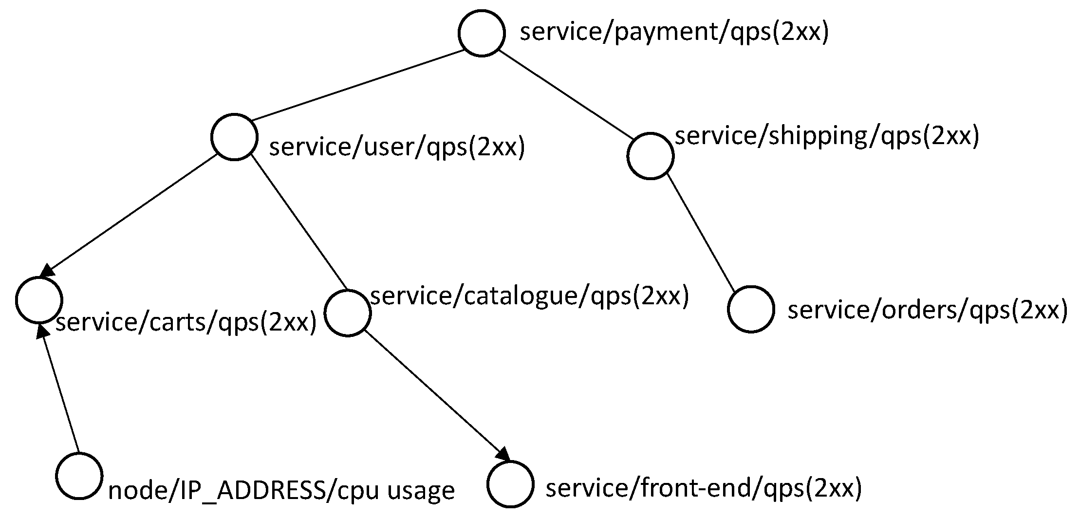
3.3. Ranking for the Causal Influence Graph

In the previous sections, we describe how to construct the causality graph. In this section, we discuss how to mine the candidate root cause paths by ranking with weight.

To determine the effects of correlation, such as $X\to Y$, we need to check whether there exists a significant value change on the time series Y after an event X happens, and we can assign a weight to the edge $X\to Y$ for measuring how much X influences Y.

Next, we describe how to assign weights to edges. There are two main steps:

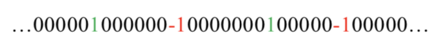
• Effectively represent the value changes for all the nodes during time period t; the value change events of a node could be denoted as a binary sequence E.
• Calculate the Pearson correlation coefficient as the weight between two sequences $E_X$ and $E_Y$, where $E_X$ is the value changes for node X, and $E_Y$ is the value changes for node Y.

To check whether there exists a significant value increase (or decrease) on a time series KPI, a t-test is adopted according to Luo’s research [28]. Given an event type denoted as E, the timestamps of the events could be denoted as $T_E=(t_1,t_2,\dots ,t_n)$, where n is the number of events that happened. A collection for the time series KPI is denoted as $S=(s_1,s_2,\dots ,s_m)$, where m is the number of points in the time series. Let ${\phi }_k^{front}(S,e_i)$ be a subseries of a KPI series S before an event $e_i$ happens with length k, and then ${\phi }_k^{rear}(S,e_i),i=1,2,\dots ,n$ is a subseries of S after the event $e_i$. Finally, set ${\Gamma }^{front}={\phi }_k^{front}(S,e_i),i=1,2\dots ,n$, and  ${\Gamma }^{rear}={\phi }_k^{rear}(S,e_i),i=1,2,\dots ,n$.

We used a t-test to check whether there was a significant value change from ${\Gamma }^{front}$ to ${\Gamma }^{rear}$. Then, the $t_{score}$ between ${\Gamma }^{front}$ and ${\Gamma }^{rear}$ can be calculated by

$$t_{score}=\frac{{\mu }_{{\Gamma }^{front}}-{\mu }_{{\Gamma }^{rear}}}{\sqrt{\frac{{\sigma }_{{\Gamma }^{front}}^2+{\sigma }_{{\Gamma }^{rear}}^2}{n}}}$$

(3)

where n is the window size, ${\mu }_{{\Gamma }^{front}}$ and ${\mu }_{{\Gamma }^{rear}}$ are the mean values of ${\Gamma }^{front}$ and ${\Gamma }^{rear}$, and ${\sigma }_{{\Gamma }^{front}}$ and ${\sigma }_{{\Gamma }^{rear}}$ are their variance values. If $t_{score}>v$, where v is the statistical test result for a specific $\alpha$ at $n-1$ degrees of freedom, this means that the KPIs have significantly increased or decreased between the two windows. When $t_{score}$ is positive, the KPI decreases significantly, and, when $t_{score}$ is negative, the KPI increases significantly. Figure 4 shows an example of detecting changes in a service’s KPI with the t-test method. The green dots on the performance data represent the identified KPI increases, and the red dots represent the identified KPI decreases.

We can further convert the performance change sequence to a ternary sequence, as shown in Figure 5. Among them, “0” indicates that the performance index has not changed significantly, “1” indicates that the KPI value has increased, and “–1” indicates that the KPI value has decreased. That is, the performance change series $E_i$ could be denoted as $E_i=(000001000000-10000000100000-100000)$.

Finally, for each edge in the causality graph, as shown in Equation (4), the Pearson coefficient of the two KPIs can be calculated by using the performance change sequence $E_1$ and $E_2$. This way, the correlation weight between the performance indicators is obtained from their performance changes, where $E_1$ and $E_2$ are performance change sequences, $Cov(E_1,E_2)$ is the covariance, and $Var\left(E\right)$ is the variance of the performance change sequence:

$$Weight=\frac{cov(E_1,E_2)}{\sqrt{var\left(E_1\right),var\left(E_2\right)}}$$

(4)

3.4. Root Cause Identification

The identification of the root cause can be regarded as a path search problem. There are many ways to solve this problem. In this study, we adopted a search algorithm based on a breadth-first search (BFS) algorithm; its pseudocode is shown in Algorithm 2. The main purpose of the algorithm is to create a queue that will store path(s) of type vectors, initialize the queue with the first path starting from the source, and then run a loop until the queue is not empty. It will get the frontmost path from the queue and then determine whether the last node of that path is a destination that is the vertex that has no predecessor: if true, then print the path and run a loop for all the vertices connected to the current vertex.

Algorithm 2: Casual search algorithm based on BFS method

Input: Causality graph G, Source vertex $SRC$

Output: The linked paths $LPATH$

INIT a queue Q to store the current path

INIT a temporary stack $path$ to store the current path

PUSH vertex $SRC$ to $path$

PUSH $path$ to Q

INIT a string list $LPATH$

while $Q\ne \varnothing$ do

$qpath=Dequeue\left(Q\right)$

GET the last vertex $LAST$ from $qpath$

if $LAST=SRC$ then

APPEND $SRC$ to $LPATH$

end if

if there is no predecessor of $LAST$ then

for vertex v in $path$ do

$tempStr$

$tempStr$ + “->”

$tempStr$ + v

append $tempStr$ to $LPATH$

end for

end for

for vertex v in G do

if v is not in $path$ then

PUSH v to $path$

ENQUEUE $path$ to Q

end if

end for

end while

When an O&M subject incurs an abnormal situation, the possible root causes of the abnormal situation can be deduced by the BFS-based causal search algorithm. Figure 6 is an example MSA; there is a time-out exception at microservice 3, which is the source vertex in the algorithm, and there are four possible causal paths:

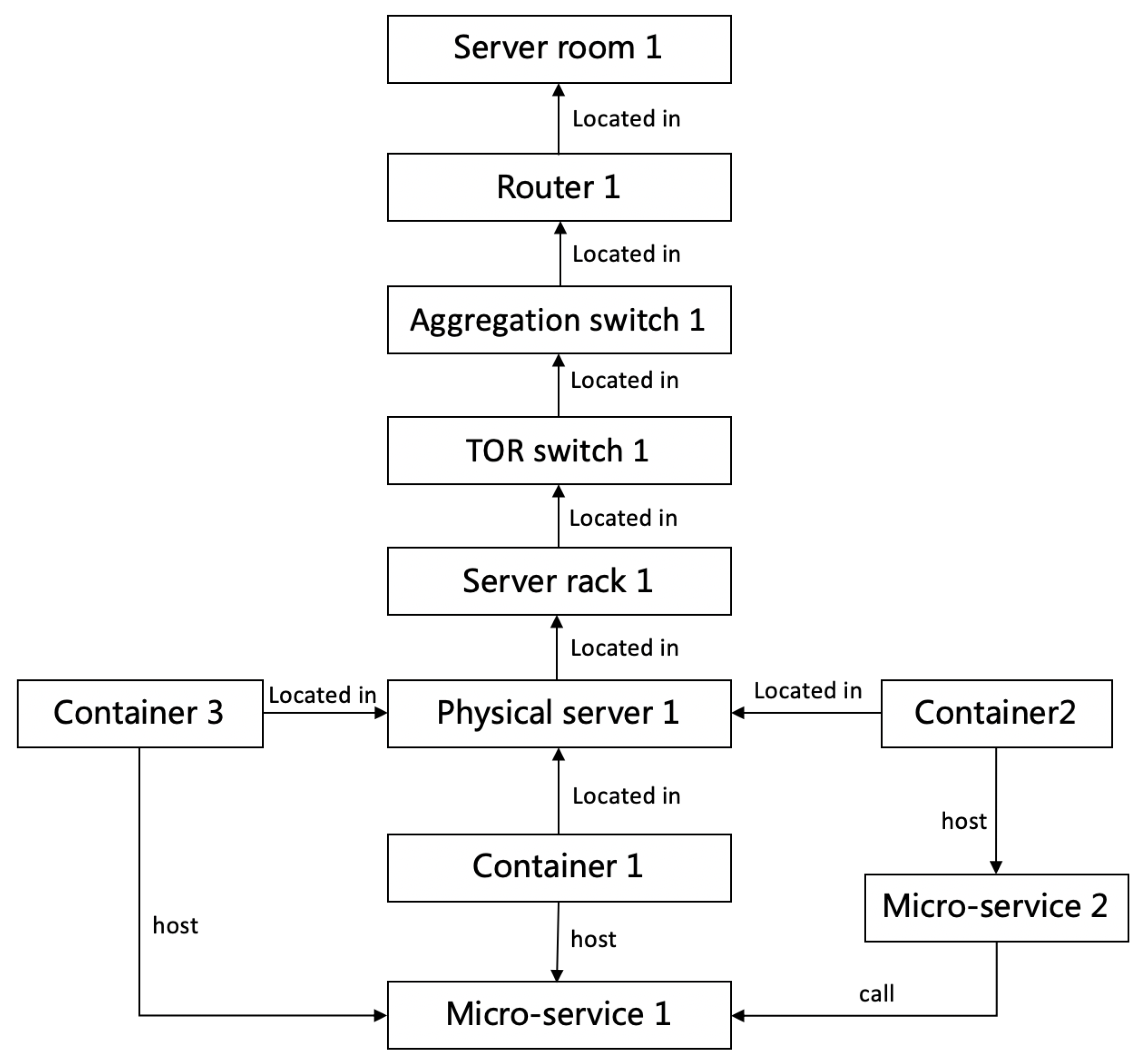
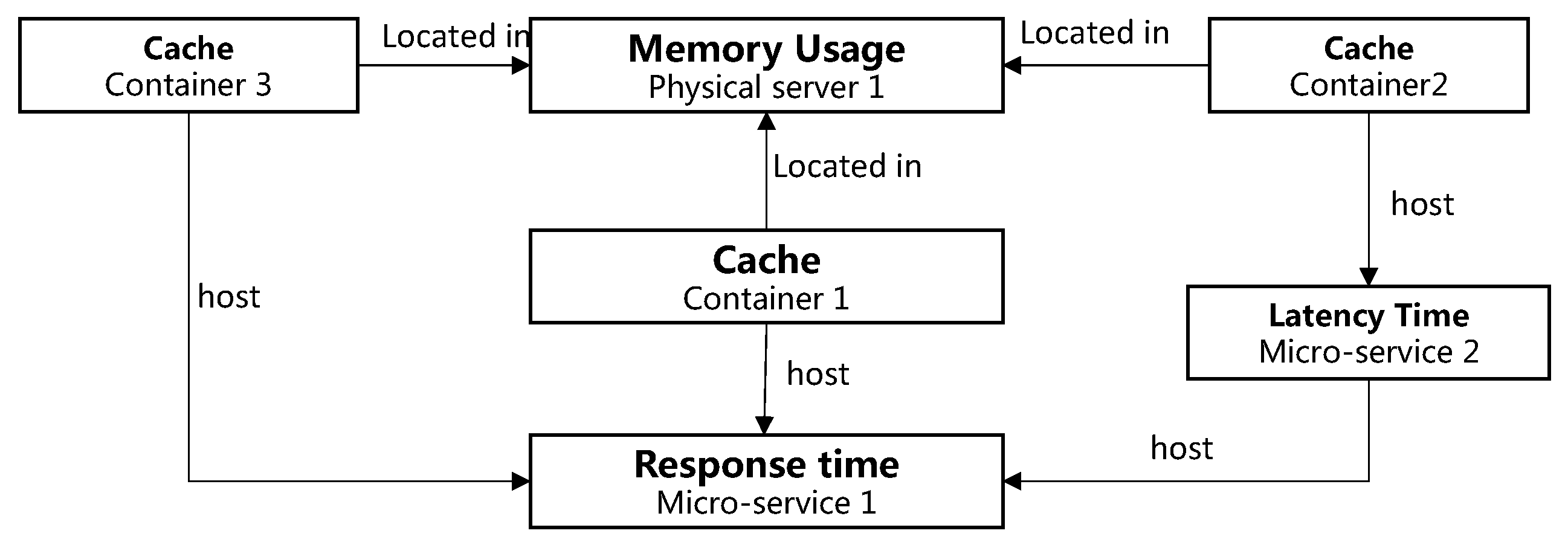
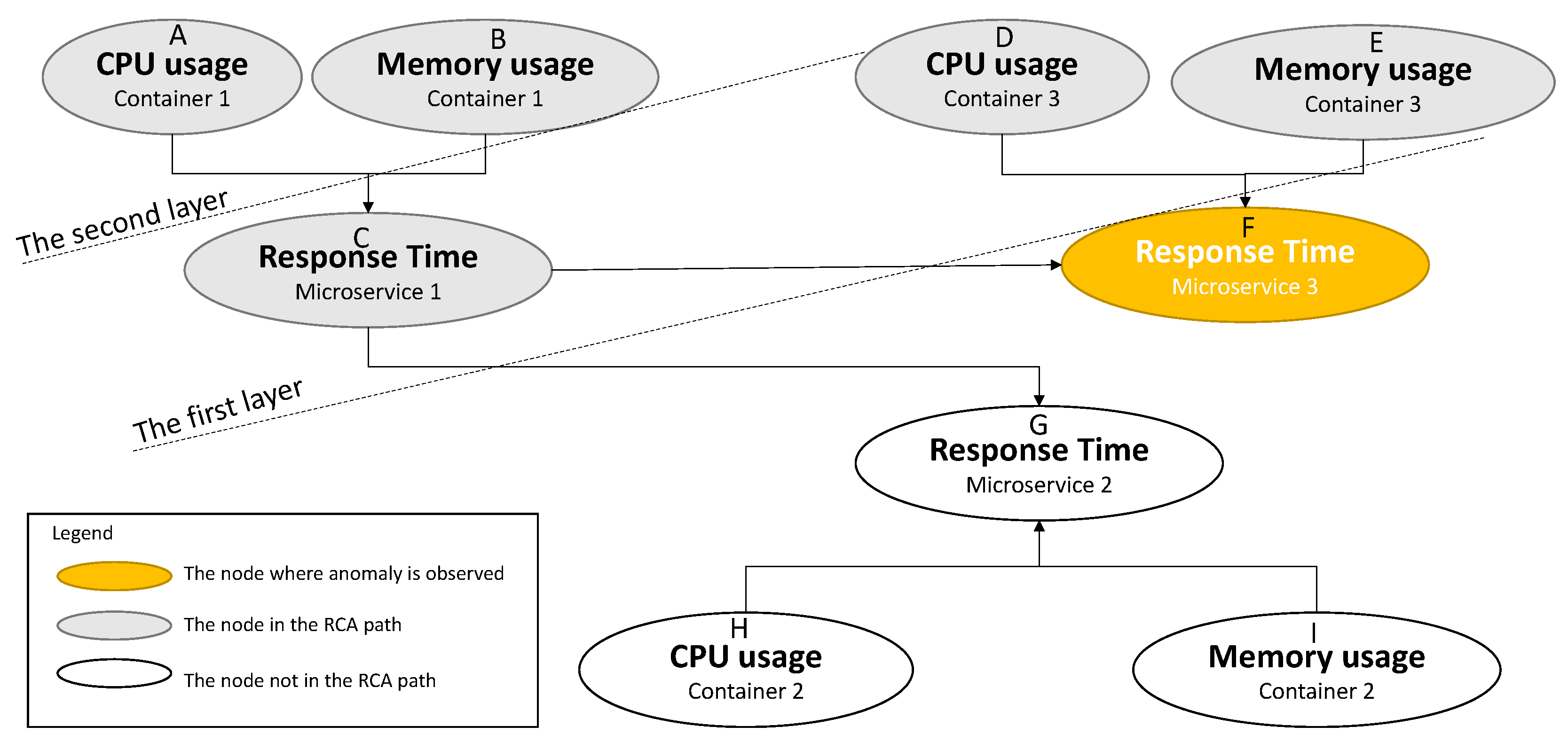
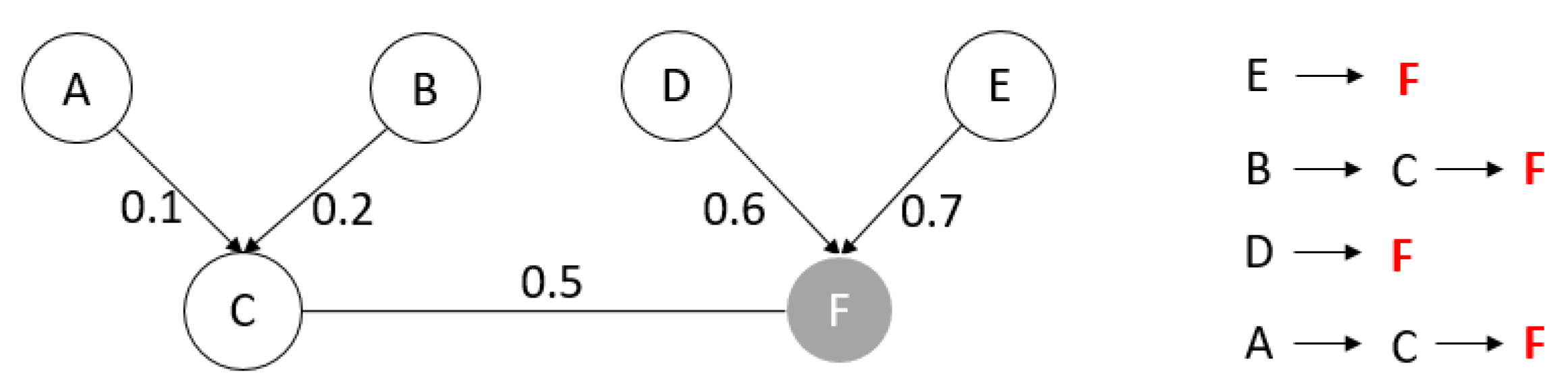
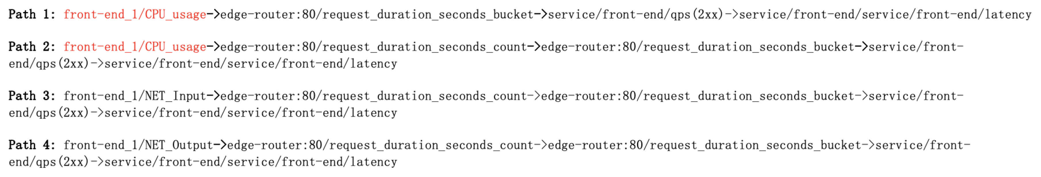
• Path 1: CPU usage of container 3 → Response time of microservice 3
• Path 2: Memory usage of container 3 → Response time of microservice 3
• Path 3: CPU usage of container 1→ Response time of micro-service 1 → Response time of microservice 3
• Path 4: Memory usage of container 1 → Response time of microservice1 → Response time of microservice 3

According to the analysis results, the time-out problem of microservice 3 might have been caused by either the high CPU or memory usage of container 3 or the high CPU or memory usage of container 1. O&M personnel can further determine the root cause of the exception by auditing the logs of container 3 and container 1.

By combining with the weight assignment method described above, the path can be sorted by rules. In this study, we sorted the paths by two rules:

• Rule 1: The sum of the weights of all edges on the path: the larger the sum, the higher the priority.
• Rule 2: The length of the path: the shorter the length, the higher the priority.

As shown in Figure 7, the highest priority of sorting is most probably the root cause path.

4. Empirical Study

This section introduces how we validate the proposed method on a classic microservice framework application named Sock Shop (https://microservices-demo.github.io). We developed a prototype that could help explore the O&M knowledge graph of the Sock Shop infrastructure, as shown in Figure 8. We also implemented the root cause search module shown in Figure 9. Finally, we did further data experimental verification for the causal search part.

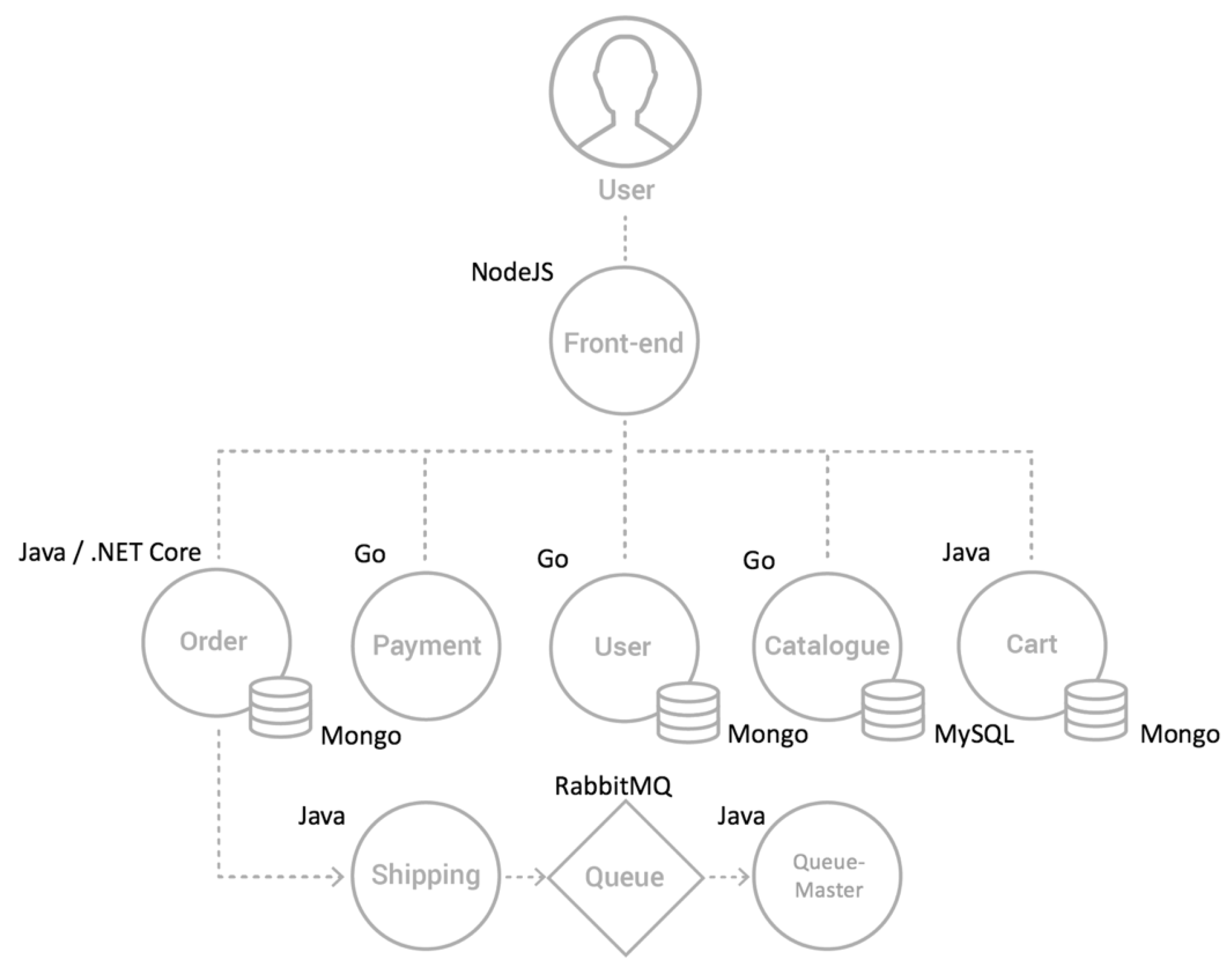
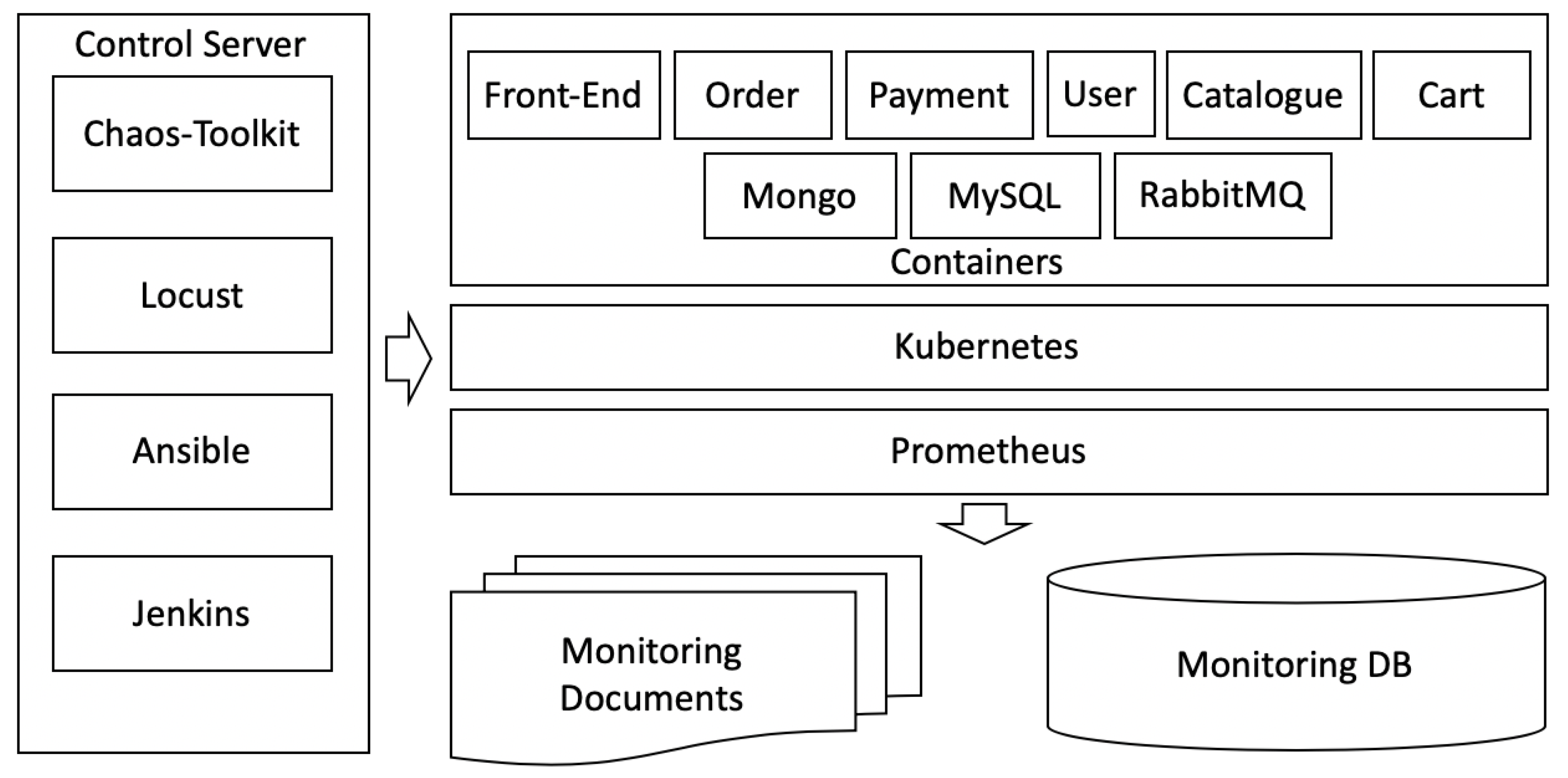
4.1. Test-Bed and Experiment Environment Setup

Sock Shop is a classic microservice application system based on Kubernetes. As Figure 10 shows, the entire Sock Shop system consists of User, Front-end, Order, Payment, Catalogue, Cart, and Shipping microservices. Each microservice can run independently and has a separate database. The implementation languages and databases of the different microservices in Sock Shop are different. The communication between microservices in Sock Shop is mainly HTTP. All service interfaces conform to the RESTful interface design style, and all services are hosted based on containers.

As shown in Figure 11, the entire deployment environment is divided mainly into the controller server and the cloud platform target test environment. We simulated the abnormal behaviors by injecting and disturbing the target cloud environment through the controller server applications. We used the chaos-testing tool Chaos Toolkit (https://chaostoolkit.org) for system disturbance, and a stress test framework Locust (https://locust.io) for the stress testing scenario. Ansible (https://www.ansible.com/) was used to do the automation task in the experiment. At the same time, various data collection tools were used in the experiment. Prometheus (https://prometheus.io) was used to collect the KPIs of microservices such as response time and throughput, Heapster (https://github.com/kubernetes-retired/heapster) was used to collect KPI data related to containers, and then Zabbix (https://www.zabbix.com) was used to collect server-related KPI data.

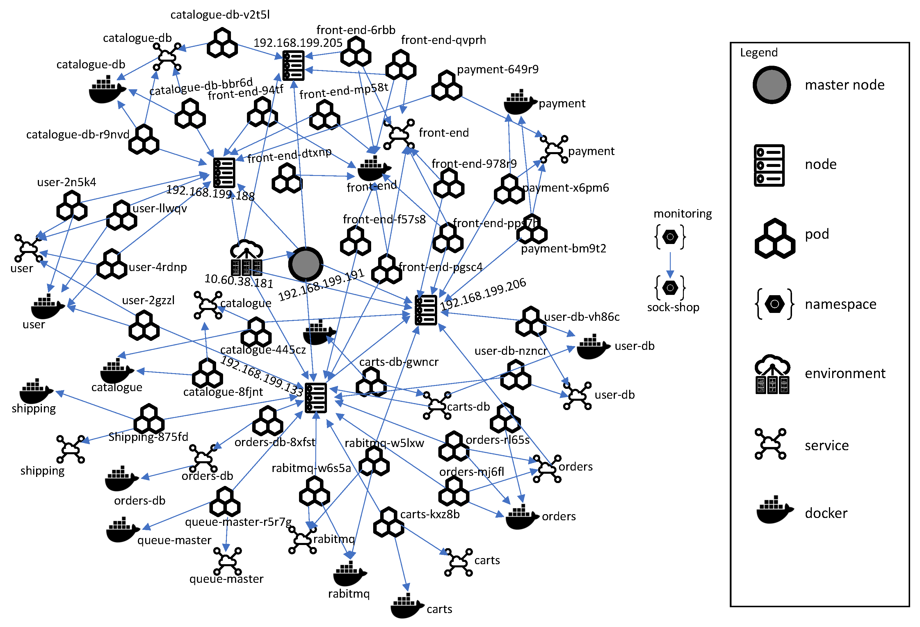
4.2. Building an O&M Knowledge Graph of the MSA System in the Kubernetes Environment

On the basis of the above deployment architecture, the knowledge graph was constructed as shown in Figure 8. The Sock Shop application was deployed in the Kubernetes cloud environment, which is commonly used in microservice architectures. In Kubernetes, Service was the core of the distributed cluster architecture. Pod was used for isolating the process that provides services for the service. It was the smallest unit on the nodes in Kubernetes, each service process was wrapped into the corresponding Pod, and a container was running in a Pod. The relation between Service and Pod in Kubernetes was implemented by Label and Label Selector. In terms of cluster management, Kubernetes divided the cluster into a master node and a group of worker nodes. Thus, the O&M knowledge graph contained at least the following subjects: Cloud Environment, Master Node, Node, Service, Pod, and Container. Their relations could be defined as follows:

• $Environment\underrightarrow{has}Node$
• $MasterNode\underrightarrow{manage}Node$
• $Pod\underrightarrow{deployed\_in}Node$
• $Pod\underrightarrow{contain}Container$
• $Pod\underrightarrow{provide}Service$
• $Service1\underrightarrow{call}Service2$
• $Service/Pod/Node\underrightarrow{ns}Namespace$
• $Service/Pod/Node\underrightarrow{profile}KPIs$

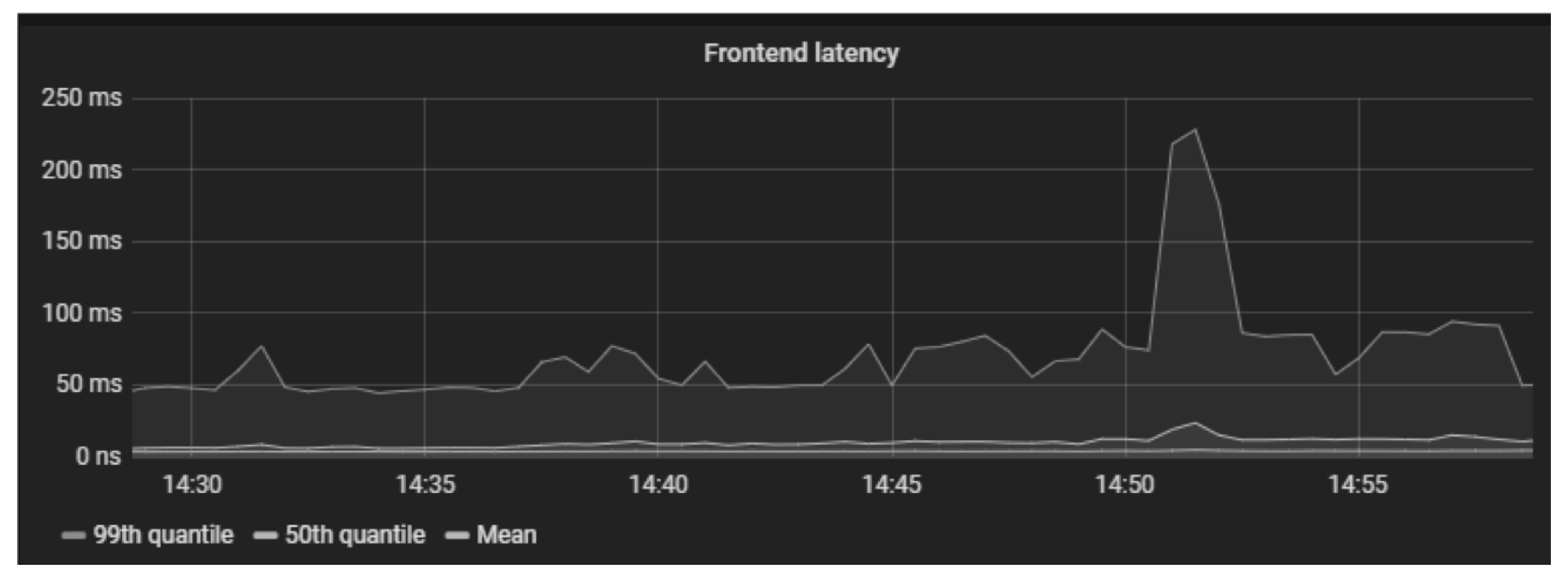
4.3. Simulation Experiment and Analysis

In this section, we tested our method from mainly two aspects: first, the executable of the causal search algorithm was tested, and then the effectiveness of the causal search algorithm was tested. In the first part, we used an example of CPU fault injection to test whether the cause and effect path output by the causal search algorithm contains the reason we expect. In the second part, to test the causal discovery performance of the proposed method, we further injected faults into several services and finally tested the performance with two metrics: precision and recall values.

4.3.1. Testing for Causality Search

In the experiment, we used chaos experimental tools to inject CPU fault injection attacks into the target environment, and set the duration of the injection to 30 min. Using fault injection, we used CPU utilization fault injection scripts on the front-end service containers. At the same time, the data of resource KPIs in the environment were collected, and the specific performance indicators were collected as shown in

Table 1. Main monitoring KPIs.

Type of Resources	KPIs	Description
Containers	CPU usage	CPU usage (%)
	MEM Usage	MEM usage (%)
	FS Read Bytes	File system read bytes (bytes/s)
	FS Write Bytes	File system write bytes (bytes/s)
	Network Input Packets	Network input packets (packets/second)
	Network Output packets	Network input packets (packets/second)
Server Nodes	CPU Usage	CPU usage (%)
	MEM Usage	Memory usage (%)
	Disk Read Bytes	Disk read bytes (bytes/s)
	Disk Write Bytes	Disk write bytes (bytes/s)
	Network Input Packets	Network input packets (packets/s)
	Network Output Packets	Network output packets (packets/s)
Services	Latency	Response per second
	QPS	Query per second (query/s)
	Success orders	Success Orders (orders/s)

.

Figure 12 shows that, after CPU fault injection into the front-end container, the latency of the front-end service of the target system changed markedly during the period from 2:50 p.m. to 2:55 p.m. Accordingly, the CPU injection fault in the experiment also occurred in this period. After collecting the system performance dataset of the chaotic experiment corresponding to Table 1, we obtained the causal relation between the performance indicators by applying the causal inference graph construction method in this study.

Because the complete graph is too large, a part of the complete graph is shown in Figure 13. Blue nodes are the KPIs of services, red nodes are the KPIs of the container, and green nodes are the KPIs of the working nodes for the Kubernetes cluster.

To diagnose the root cause of the front-end latency, we applied the causal search algorithm. The results show that the root cause chains in Figure 14 generated by the proposed algorithm are basically consistent with the actual Sock Shop system architecture and do reflect the call relations between services.

4.3.2. Effective Evaluation

To further verify the accuracy of the causal search algorithm, we referred to our previous research work. We injected more types of faults into the Sock Shop platform, which included CPU burnout, MEM overload, disk I/O block, and network jam. Meanwhile, those faults were injected into the various microservices in Sock Shop, and the number of the injected faults for each type and each service is 20. Finally, we evaluated the performance of our causality search algorithm with two evaluation metrics in Microscope [18]:

• Precision at the top K indicates the probability that the root cause in the top K of the ranking list if the cause inference is triggered.
• Recall at the top K is the portion of the total amount of real causes that were actually retrieved at the top K of the ranking list.

In our experiment, we set $K=2$. Finally, we could obtain the experimental results shown in

Table 2. Performance for different services.

	Front-End	Catalogue	User	Carts	Orders	Shipping	Payment
CPU Burnout
precision	100	85	90	80	95	60	55
recall	100	95	90	90	100	60	60
Mem Overload
precision	100	85	100	85	100	55	75
recall	100	95	100	100	100	55	75
Disk I/O Block
precision	100	95	100	90	100	55	65
recall	100	95	100	95	100	60	65
Network Jam
precision	100	100	100	85	100	70	55
recall	100	100	100	100	100	70	65

.

The results in Table 2 show the precision and recall values of the root cause search algorithm in various services. The table shows that, except for Shipping and Payment, the precision and recall values of the services were above 80%. The main reason for the poor performance of the Shipping and Payment services is that those services were not highly dependent on other services and were not computationally intensive, even in the case of stress testing.

Finally, we further evaluated the performance overhead of our method based on the above Sock Shop experiment. The evaluation experiment was conducted on one physical server (DELL R730) which was equipped with 2x Intel Xeon CPU E5-2630 v4 @ 2.10 GHz, 128 G of RAM. In the above experiment, we collected monitoring records that contained more than 100 KPIs; then, we measured the resource and time overhead of our method in terms of different data volumes and different numbers of KPIs. As shown in

Table 3. Overhead of the experiment.

Number of KPIs	20			50			100
Resource Usage/ Rows of Records	Time (s)	CPU (%)	MEM (MB)	Time (s)	CPU (%)	MEM (MB)	Time (s)	CPU (%)	MEM (MB)
25	4.36	7.92	17.92	10.46	7.94	34.19	15.18	8.56	33.86
50	4.38	7.72	18.71	12.55	8.89	36.65	25.41	8.72	35.77
100	4.50	7.49	18.93	17.42	7.42	35.47	32.61	8.86	37.68
150	4.36	8.99	19.17	16.71	7.53	39.45	31.07	8.43	38.51
200	4.49	7.67	19.66	17.79	7.45	38.09	32.71	8.56	40.56
250	4.50	7.03	19.71	17.81	7.57	38.91	34.41	8.67	39.73
500	4.38	7.13	19.78	18.81	8.09	39.43	35.74	8.98	41.43
750	4.49	7.02	21.12	20.11	8.92	39.56	35.69	9.12	43.40
1000	4.40	7.67	21.29	20.43	8.01	39.84	37.88	9.43	44.99
1500	4.43	7.23	21.89	20.53	8.37	40.94	40.95	9.67	46.83
2000	4.45	7.37	22.07	27.19	8.85	43.37	43.39	9.77	49.33

, we analyzed the performance consumption of causality graph construction and causality search for 20, 50, and 100 KPIs, respectively, and considered the comparison of performance consumption under different conditions from 25 to 2000 records. Obviously, the computing time and resource consumption also continued to increase as the number of KPIs increased. However, as far as we know, this problem can be improved by introducing parallel computing to the PC algorithm [29].

5. Conclusions

In this paper, to solve the problem of diagnosing the root cause of abnormal performance in cloud applications of MSAs, we propose an RCA method based on a knowledge graph and a causal search algorithm. The paper describes how to construct an O&M knowledge graph and further improves a causal search algorithm based on the PC algorithm and in turn based on an O&M knowledge graph. Through experiments, we found that the proposed method can successfully generate a causality graph and output possible root cause paths. We also experimentally evaluated the performance of the method. For most services, both the recall and precision of the algorithm exceeded 80% for most scenarios.

There are still many places that can be optimized in this paper. The following summarizes such future work.

Firstly, the current causality graph is constructed without considering external factors. When a certain external factor causes an anomaly, the observed node affected by the external factor shows a highly correlated metric pattern in the anomaly time window. A pseudo-anomaly clustering algorithm [1] could be employed to solve such problems, and we will consider this part in future work.

Secondly, the runtime of the PC algorithm is time-consuming due to the large number of KPIs. A parallel computing technique for the PC algorithm could be considered to improve the performance.

In addition, we will strengthen the comparison experiment and enrich the prototype tool in this study. On the one hand, we have not reproduced the results of current related papers, so we will further strengthen the comparison between our method and other methods to further verify the advantages of our method. On the other hand, we have developed only a simple prototype tool to test our method: there are still many features that need to be improved. For example, in order to ensure the practicability of the proposed method, we must solve the problem of synchronously updating the knowledge graph as the microservice deployment changes. We can monitor the deployment changes of the environment by calling on the Kubernetes API to trigger the update of the knowledge graph synchronously. Only in this way can we ensure that the causality graph construction and search are conducted based on the latest knowledge graph. In brief, we will further improve the knowledge graph tool and further enrich the prototype tool, making our method more applicable.

References

1. Kim, M.; Roshan, S.; Sam, S. Root Cause Detection in a Service-Ooriented Architecture; ACM SIGMETRICS Performance Evaluation Review 41.1; ACM: New York, NY, USA, 2013; pp. 93–104. [Google Scholar]
2. Thalheim, J.; Rodrigues, A.; Akkus, I.E.; Bhatotia, P.; Chen, R.; Viswanath, B.; Jiao, L.; Fetzer, C. Sieve: Actionable insights from monitored metrics in distributed systems. In Proceedings of the 18th ACM/IFIP/USENIX Middleware Conference, Las Vegas, NV, USA, 11–15 December 2017. [Google Scholar]
3. Weng, J.; Wang, J.H.; Yang, J.; Yang, Y. Root cause analysis of anomalies of multitier services in public clouds. IEEE/ACM Trans. Netw. 2018, 26, 1646–1659. [Google Scholar] [CrossRef]
4. Marwede, N.; Rohr, M.; van Hoorn, A.; Hasselbring, W. Automatic failure diagnosis support in distributed large-scale software systems based on timing behavior anomaly correlation. In Proceedings of the IEEE 2009 13th European Conference on Software Maintenance and Reengineering, Kaiserslautern, Germany, 24–27 March 2009. [Google Scholar]
5. Marvasti, M.A.; Poghosyan, A.; Harutyunyan, A.N.; Grigoryan, N. An anomaly event correlation engine: Identifying root causes, bottlenecks, and black swans in IT environments. VMware Tech. J. 2013, 2, 35–45. [Google Scholar]
6. Zeng, C.; Tang, L.; Li, T.; Shwartz, L.; Grabarnik, G.Y. Mining temporal lag from fluctuating events for correlation and root cause analysis. In Proceedings of the IEEE 10th International Conference on Network and Service Management (CNSM) and Workshop, Rio de Janeiro, Brazil, 17–21 November 2014. [Google Scholar]
7. Lin, Q.; Zhang, H.; Lou, J.-G.; Zhang, Y.; Chen, X. Log clustering based problem identification for online service systems. In Proceedings of the 2016 IEEE/ACM 38th International Conference on Software Engineering Companion (ICSE-C), Austin, TX, USA, 14–22 May 2016. [Google Scholar]
8. Jia, T.; Chen, P.; Yang, L.; Meng, F.; Xu, J. An approach for anomaly diagnosis based on hybrid graph model with logs for distributed services. In Proceedings of the 2017 IEEE International Conference on Web Services (ICWS), Honolulu, HI, USA, 25–30 June 2017. [Google Scholar]
9. Xu, J.; Chen, P.; Yang, L.; Meng, F.; Wang, P. LogDC: Problem diagnosis for declartively-deployed cloud applications with log. In Proceedings of the 2017 IEEE 14th International Conference on e-Business Engineering (ICEBE), Shanghai, China, 4–6 November 2017. [Google Scholar]
10. Xu, X.; Zhu, L.; Weber, I.; Bass, L.; Sun, D. POD-diagnosis: Error diagnosis of sporadic operations on cloud applications. In Proceedings of the 2014 44th Annual IEEE/IFIP International Conference on Dependable Systems and Networks, Atlanta, GA, USA, 23–26 June 2014. [Google Scholar]
11. Jia, T.; Yang, L.; Chen, P.; Li, Y.; Meng, F.; Xu, J. Logsed: Anomaly diagnosis through mining time-weighted control flow graph in logs. In Proceedings of the 2017 IEEE 10th International Conference on Cloud Computing (CLOUD), Honolulu, CA, USA, 25–30 June 2017. [Google Scholar]
12. Mi, H.; Wang, H.; Cai, H.; Zhou, Y.; Lyu, M.R.; Chen, Z. P-tracer: Path-based performance profiling in cloud computing systems. In Proceedings of the 2012 IEEE 36th Annual Computer Software and Applications Conference, Izmir, Turkey, 16–20 July 2012. [Google Scholar]
13. Chen, M.Y.; Kiciman, E.; Fratkin, E.; Fox, A.; Brewer, E. Pinpoint: Problem determination in large, dynamic internet services. In Proceedings of the Proceedings International Conference on Dependable Systems and Networks, Washington, DC, USA, 23–26 June 2002. [Google Scholar]
14. Gao, H.; Yang, Z.; Bhimani, J.; Wang, T.; Wang, J.; Sheng, B.; Mi, N. AutoPath: Harnessing parallel execution paths for efficient resource allocation in multi-stage big data frameworks. In Proceedings of the 2017 26th International Conference on Computer Communication and Networks (ICCCN), Vancouver, BC, Canada, 31 July–3 August 2017. [Google Scholar]
15. Di Pietro, R.; Lombardi, F.; Signorini, M. CloRExPa: Cloud resilience via execution path analysis. Future Gener. Comput. Syst. 2014, 32, 168–179. [Google Scholar] [CrossRef]
16. Pengfei, C.; Yong, Q.; Pengfei, Z.; Di, H. CauseInfer: Automatic and distributed performance diagnosis with hierarchical causality graph in large distributed systems. In Proceedings of the IEEE Conference on Computer Communications, Toronto, ON, Canada, 27 April–2 May 2014. [Google Scholar]
17. Pengfei, C.; Yong, Q.; Di, H. CauseInfer: Automated end-to-end performance diagnosis with hierarchical causality graph in cloud environment. IEEE Trans. Serv. Comput. 2016, 12, 214–230. [Google Scholar]
18. Lin, J.; Pengfei, C.; Zibin, Z. Microscope: Pinpoint performance issues with causal graphs in micro-service environments. In Proceedings of the International Conference on Service-Oriented Computing, Hangzhou, China, 12–15 November 2018; Springer: Cham, Switzerland, 2018. [Google Scholar]
19. Ping, W.; Jingmin, X.; Meng, M.; Weilan, L.; Disheng, P.; Yuan, W.; Pengfei, C. Cloudranger: Root cause identification for cloud native systems. In Proceedings of the 2018 18th IEEE/ACM International Symposium on Cluster, Cloud and Grid Computing (CCGRID), Washington, DC, USA, 1–4 May 2018. [Google Scholar]
20. Nie, X.; Zhao, Y.; Sui, K.; Pei, D.; Chen, Y.; Qu, X.; Zhao, Y.; Sui, K.; Pei, D.; Chen, Y.; et al. Mining causality graph for automatic web-based service diagnosis. In Proceedings of the 2016 IEEE 35th International Performance Computing and Communications Conference (IPCCC), Las Vegas, NV, USA, 9–11 December 2016. [Google Scholar]
21. Lin, W.; Ma, M.; Pan, D.; Wang, P. FacGraph: Frequent anomaly correlation graph mining for root cause diagnose in MSA. In Proceedings of the 2018 IEEE 37th International Performance Computing and Communications Conference (IPCCC), Orlando, FL, USA, 17–19 November 2018. [Google Scholar]
22. Hirochika, A.; Fukuda, K.; Abry, P.; Borgnat, P. Network application profiling with traffic causality graphs. Int. J. Netw. Manag. 2014, 24, 289–303. [Google Scholar]
23. Abele, L.; Anic, M.; Gutmann, T.; Folmer, J.; Kleinsteuber, M.; Vogel-Heuser, B. Combining knowledge modeling and machine learning for alarm root cause analysis. IFAC Proc. Vol. 2013, 46, 1843–1848. [Google Scholar] [CrossRef] [Green Version]
24. Qiu, J.; Qingfeng, D.; Chongshu, Q. KPI-TSAD: A Time-Series Anomaly Detector for KPI Monitoring in Cloud Applications. Symmetry 2019, 11, 1350. [Google Scholar] [CrossRef] [Green Version]
25. Spirtes, P.; Glymour, C. An algorithm for fast recovery of sparse causal graphs. Soc. Sci. Comput. Rev. 1991, 9, 62–72. [Google Scholar] [CrossRef] [Green Version]
26. Heim, P.; Hellmann, S.; Lehmann, J.; Lohmann, S.; Stegemann, T. RelFinder: Revealing relationships in RDF knowledge bases. In Proceedings of the International Conference on Semantic and Digital Media Technologies, Graz, Austria, 2–4 December 2009; Springer: Berlin/Heidelberg, Germany, 2009. [Google Scholar]
27. Neuberg, L.G. Causality: Models, reasoning, and inference, by judea pearl, cambridge university press, 2000. Econom. Theory 2003, 19, 675–685. [Google Scholar] [CrossRef]
28. Luo, C.; Lou, J.-G.; Lin, Q.; Fu, Q.; Ding, R.; Zhang, D.; Wang, Z. Correlating events with time series for incident diagnosis. In Proceedings of the 20th ACM SIGKDD International Conference on Knowledge Discovery and Data Mining, New York, NY, USA, 24–27 August 2014. [Google Scholar]
29. Le, T.D.; Hoang, T.; Li, J.; Liu, L.; Liu, H.; Hu, S. A fast PC algorithm for high dimensional causal discovery with multi-core PCs. IEEE/ACM Trans. Comput. Biol. Bioinform. 2016, 16. [Google Scholar] [CrossRef] [PubMed] [Green Version]
Figure 1. Framework of the proposed method.
Applsci 10 02166 g001
Figure 2. Sample knowledge graph of software and hardware subjects for an MSA application.
Applsci 10 02166 g002
Figure 3. Sample knowledge graph for KPIs from monitoring targets.
Applsci 10 02166 g003
Figure 4. Performance changes identification by t-test.
Applsci 10 02166 g004
Figure 5. Performance change ternary sequence.
Applsci 10 02166 g005
Figure 6. A root cause tracing example for performance anomaly.
Applsci 10 02166 g006
Figure 7. Root cause identification with weight priority.
Applsci 10 02166 g007
Figure 8. Explore function O&M knowledge graph in the prototype.
Applsci 10 02166 g008
Figure 9. Causality search function in the prototype.
Applsci 10 02166 g009
Figure 10. Sock Shop architecture.
Applsci 10 02166 g010
Figure 11. Deployment architecture of the whole experiment environment.
Applsci 10 02166 g011
Figure 12. Front-end latency after CPU fault injection.
Applsci 10 02166 g012
Figure 13. Part of causality graph for all performance indicators.
Applsci 10 02166 g013
Figure 14. Root cause chain paths of the experiment.
Applsci 10 02166 g014