A Method of On-Site Describing the Positional Relation between Two Horizontal Parallel Surfaces and Two Vertical Parallel Surfaces

Abstract

The position error of two parallel surfaces is generally constrained by parallelism. However, as a range of change, it cannot represent the positional relation between two parallel surfaces. Large-scale equipment such as machine tools are complex and difficult to move. It is also an engineering problem to perform field measurements on it. To this end, a method of describing the positional relation between two horizontal parallel surfaces and two vertical parallel surfaces on-site is proposed in this paper, which is a novel kind of position error, enriching the form of parallel surface position error, and solves the inconvenience problem of large equipment position error measurement. The measurement mechanisms are designed, and the measurement principle is given. Firstly, the combined projection waveform of the measured surface can be obtained by the geometric relationship between the measurement mechanism and the measured surface. Secondly, an algorithm is studied to process the obtained waveform, and the combined projection curve of the measured surface is acquired. Then, under the condition of considering the shape contours of the two surfaces, an algorithm is developed to acquire the calculated shape contour of the measured surface. According to the difference between the calculated surface shape contour and the known shape contour of the measured surface, the positional relation of the two surfaces can be determined. Meanwhile, the mathematical models of algorithms are established, and the measurement experiments are carried out, and the algorithms are verified by the mutual measurement method of the two surfaces. The results show that this method can accurately obtain the positional relation of two horizontal parallel surfaces and two vertical parallel surfaces.

1. Introduction

The CNC machine tool is an important piece of equipment in the traditional manufacturing industry. Two positioning surfaces of the machine tool serve as the datum surface for the mounting rails, and their position error plays a vital role in the accuracy of the machine tool. In the modern manufacturing industry, the position error of two parallel surfaces is generally constrained by parallelism, and parallelism is orientation error, which is the total allowable variation of the measured element in the direction relative to the datum. Therefore, the orientation error has the function of controlling the direction, that is, controlling the direction of the measured elements relative to the datum elements. However, the calculation method of parallelism is very mature. Firstly, we need to establish a datum direction on the datum plane. The method is to fit a straight line (as shown in Figure 1a) or a surface (as shown in Figure 1b) as a datum direction. The obtained parallelism is a number. The key to parallelism evaluation is to determine the datum direction.

With the development of the manufacturing industry, the requirements for machine tools are increasing. In order to improve the performance of the machine tool, we study the impact of the positioning accuracy of the machine tool on the accuracy of the machined parts and maintain the accuracy of the machine tool itself. The more we know about position errors, the better for us. Therefore, this paper proposes a method of describing the positional relation between two parallel surfaces on-site, which is a novel kind of position error. It has no datum direction, enriching the form of parallel surface position error. The significance of obtaining the positional relation curve of the two positioning surfaces on the machine tool is that, on one hand, the positional relation curve can guide the subsequent modification, grinding, bed fitting and quantitative analysis of the machined parts. On the other hand, the positional relation curve can also be used to evaluate the torsional state of the surface.

In the development of shape error detection methods, there are several novel methods are used to obtain straightness [1,2,3,4], flatness [5,6,7,8,9,10], roundness [11,12]. However, because the method of evaluating the parallelism in position error is relatively simple, there is relatively little research on this aspect. Hsieh et al. [13] proposed a method for measuring the parallelism of static and dynamic linear guideways. Hwang et al. [14] proposed a three-probe system, which can be used to acquire the parallelism and straightness of a pair of guideways simultaneously. The parallelism measurements are based on an expanded reversal method and the straightness measurements are based on a sequential two-point method. Bhattacharya et al. [15] described an interferometric method for measuring the parallelism of an end face of a transparent material. Lee et al. [16] developed a double ball-bar method to measure parallelism errors of the spindle axis of machine tools. Maurizio et al. [17] discussed two methods for measuring the parallelism error of gauge blocks. It can be known from searching literatures that in the study of shape and position errors, there is very little description of the positional relation between two parallel surfaces. Moreover, the above methods need to be carried out using specific equipment and in a specific environment, and the layout of the measurement mechanism is very complex and needs enough space, but the operating space of machine tools is often limited. Especially for two vertical surfaces, it is more difficult to perform field measurement. However, Jywe et al. [18] performed an online measurement of the machine tool’s two-axis straightness error. Hsien et al. [19] designed an online measurement system for measuring the linearity and parallelism of linear guides. Unfortunately, these two measurement systems cannot measure the positional relation of two parallel surfaces.

The parallelism measurement in industry commonly uses specific tools, such as micrometer, deflection instrument, coordinate measuring machines etc. In fact, micrometer has great randomness, which is greatly influenced by the operator’s proficiency and experience. In the detection process, the operator can only judge the quality by observing the change range of the micrometer, and the detection data cannot be directly saved to the computer. The coordinate measuring machine can record the test data with high precision, but it can’t measure the machine tool and large equipment on site. Therefore, from the above introduction, for machine tools with limited operating space, developing a simple and easy-to-operate measuring instrument will be an effective method to on-site obtain the positional relation of two positioning surfaces.

In this paper, a method of describing the positional relation of the two horizontal parallel surfaces and two vertical parallel surfaces on-site is proposed. This method can separate the shape contours of the two surfaces and obtain the real positional relation curve of the two surfaces. At the same time, the laser displacement sensor, which can record the detection data to the computer, is selected as the detection element, a continuous measuring mechanism suitable for manual operation is developed, and the corresponding algorithms are studied. Finally, the calculation results are drawn into a curve, which makes the description of the positional relation more intuitive. This method can also be used to measure two working surfaces and two guideways of large equipment.

The rest of this paper is organized as follows. In Section 2 the principle of the measurement mechanism is depicted. In Section 3, the method for describing the positional relation between two surfaces is introduced. In Section 4, mathematical models of the algorithms are established. In Section 5, the measurement experiment is carried out and the results are analyzed. Finally, a conclusion is given in Section 6.

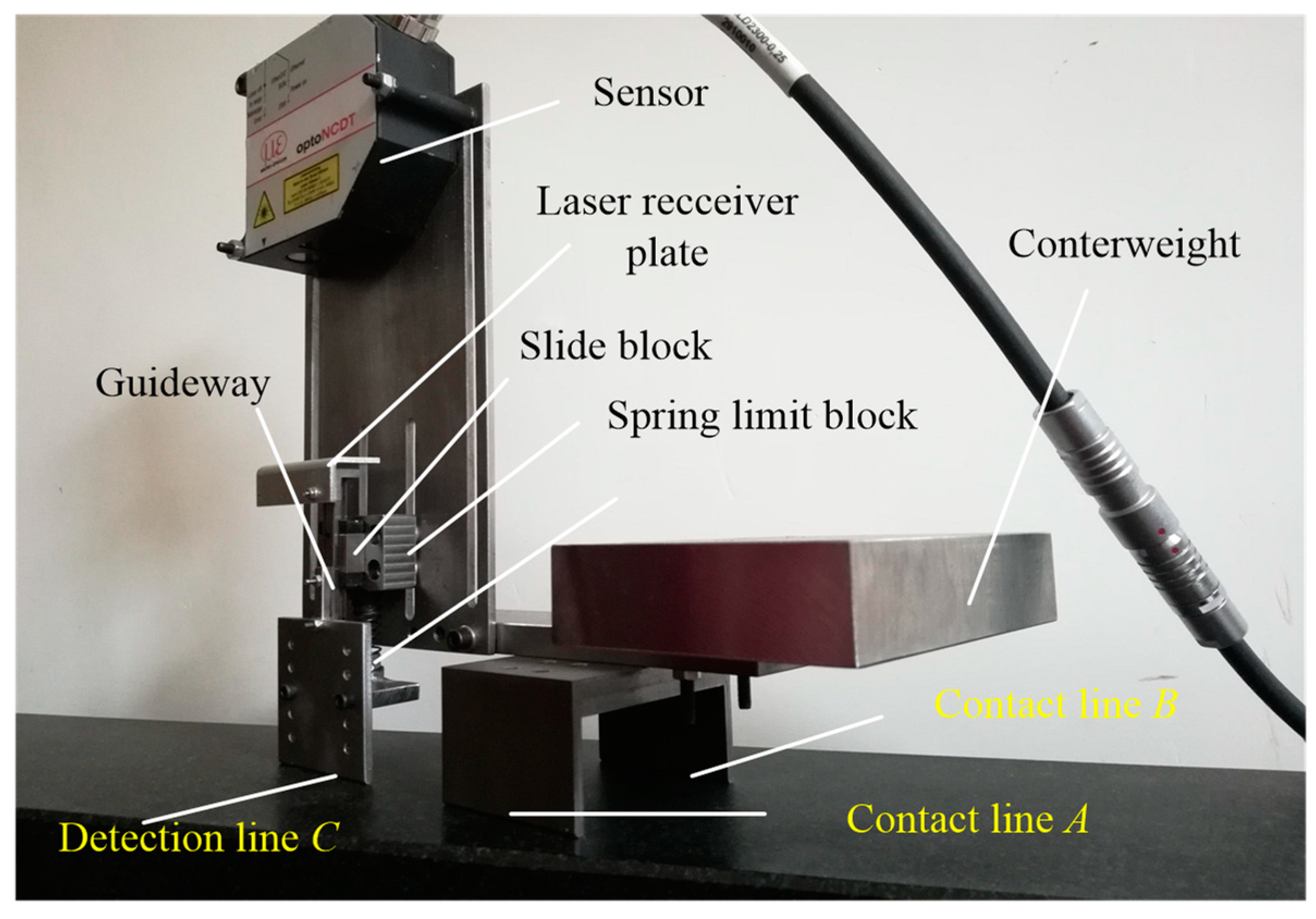
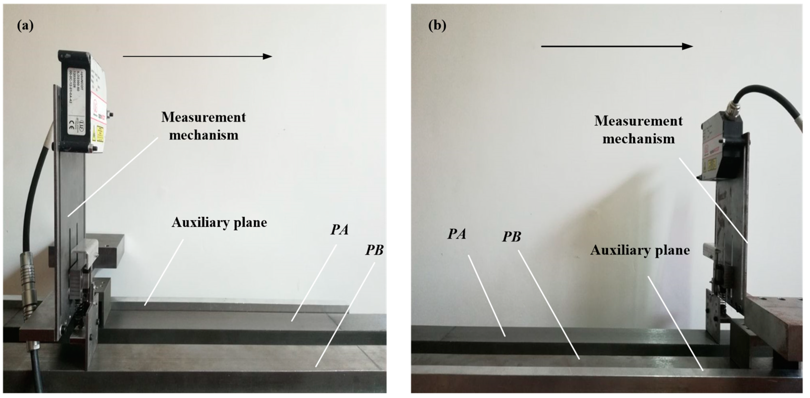
2. Principle of the Measurement Mechanism

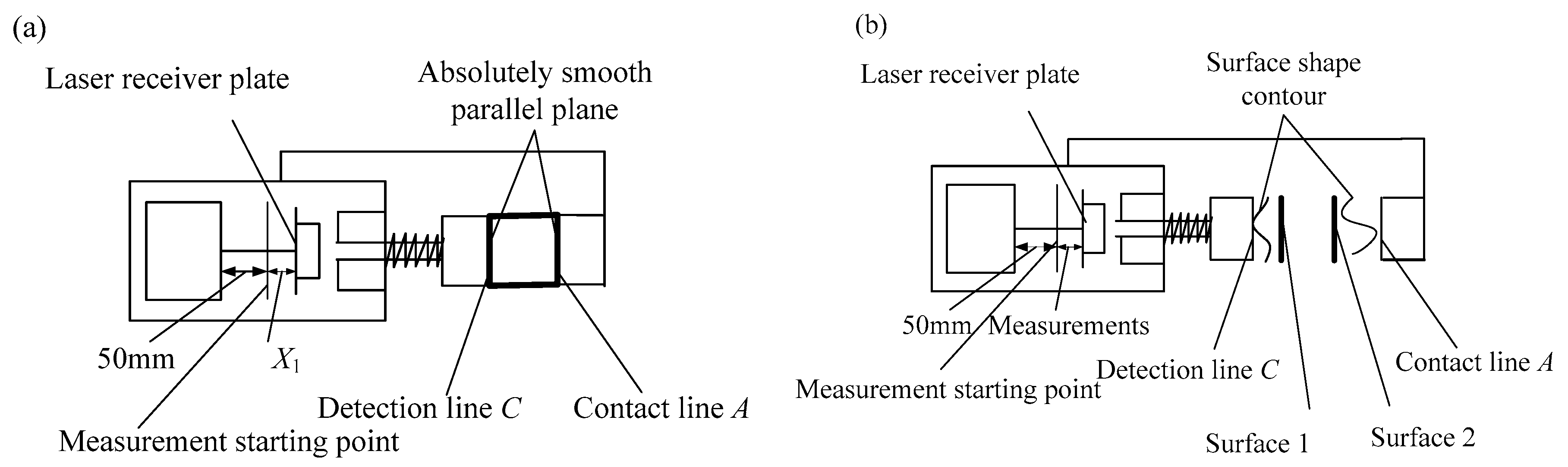
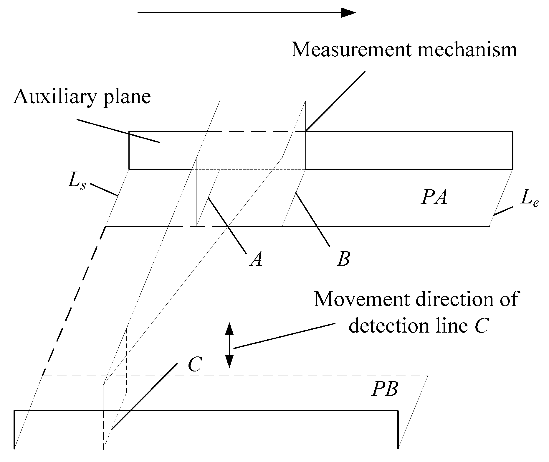
2.1. Measuring Mechanism for Measuring Two Horizontal Parallel Surfaces

Figure 2 shows the measurement mechanism for measuring the positional relation between two horizontal parallel surfaces. The laser displacement sensor (triangulation) ILD-2300 is selected as the detection element and the technical parameters of the sensor are shown in

Table 1. Laser displacement sensor parameters.

Model	Parameter
Frequency	20 kHz
Resolution	0.3 μm
Absolute error	4 μm (≤±0.02%) full scale
Starting measurement range	50 mm
Light source	semiconductor laser (1 mW, 670 nm red)
Impact resistance	15 g/6 ms
Operating temperature	0–50 °C
Power requirements	24 VDC (11…30 VDC), Max 150 mA
Security Level	Class 2 according to DIN EN 60825-1: 2001-11
Spot diameter	SMR140 × 200 μm, MMR46 × 45 μm, EMR140 × 200 μm

.

The measurement mechanism consists of slider, guideway, spring limit block, laser receiving plate, counterweight block, spring, contact line A and B, and detection line C. The length of contact line A, B and detection line C are 50 mm, and the distance between contact line A and detection line C is 60 mm. The contact line A, B and detection line C are ground after processing, and the processing accuracy grade is IT3.The measurement mechanism is in equilibrium with the counterweight, and contact lines A and B are fixed contact lines. Detection line C is connected with the measurement mechanism through micro-guideway and springs, the slider block is fixed on the measurement mechanism, the laser receiving plate is integrated with the micro-guideway and detection line C. In the process of measurement, the measurement mechanism is manually driven to move in a fixed direction, under the function of the spring, the detection line C fluctuates up and down with the change of shape contour the measured surface, the fluctuation is transmitted to the laser receiving plate through the micro-guideway. At this time, the laser displacement sensor detects the fluctuation and the computer records the measurements.

It is known that the surface contour consists of roughness contour, waviness contour and surface shape contour. The surface shape contour is macroscopic. In this paper, the three-dimensional shape of the measured surface is projected on a plane perpendicular to it, and the macroscopic contour curve obtained is the surface shape contour, as shown in Figure 3. Therefore, the motion trajectories of the contact lines A, B, and detection lines C are surface shape contour.

As shown in Figure 4a, according to Table 1, the initial measuring range is 50 mm. When the detection line C and the contact line A are collinear, the detection data should be a fixed value, defining it as the initial value X₀. When considering the shape contours of the two surfaces, the position of the detection line C may change, as shown in Figure 4b. The difference between the measurements and the initial value is the displacement of the detection line C relative to the contact line A.

The advantage of this mechanism is that it easy to operate, and suitable for field measurement. It can continuously obtain the stored data which change with the shape contour of the measured surface, instead of some discrete points on the same straight line along the measuring direction. Meanwhile, it can separate the shape contours of the two surfaces, which cannot be achieved by ordinary testing equipment.

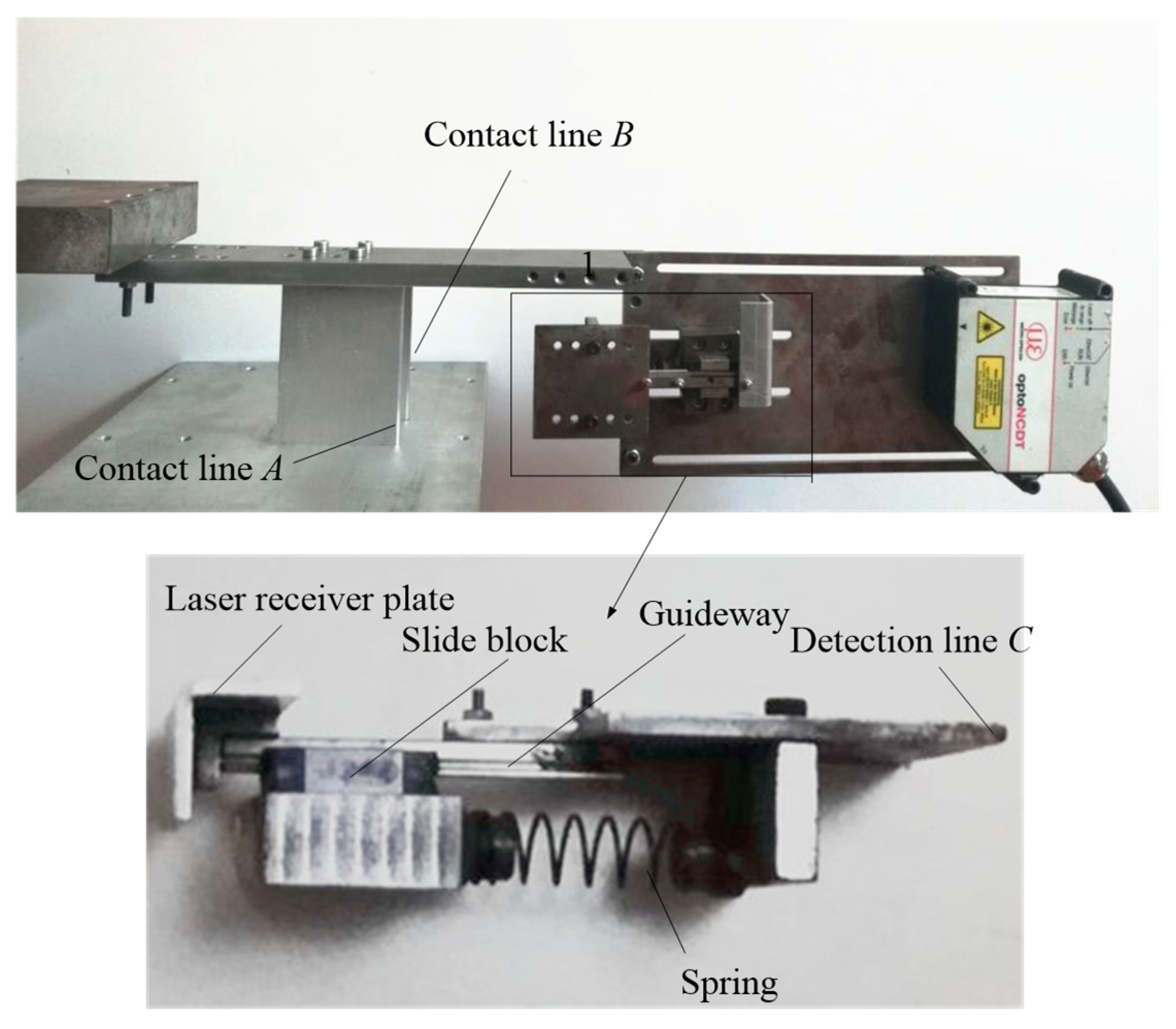
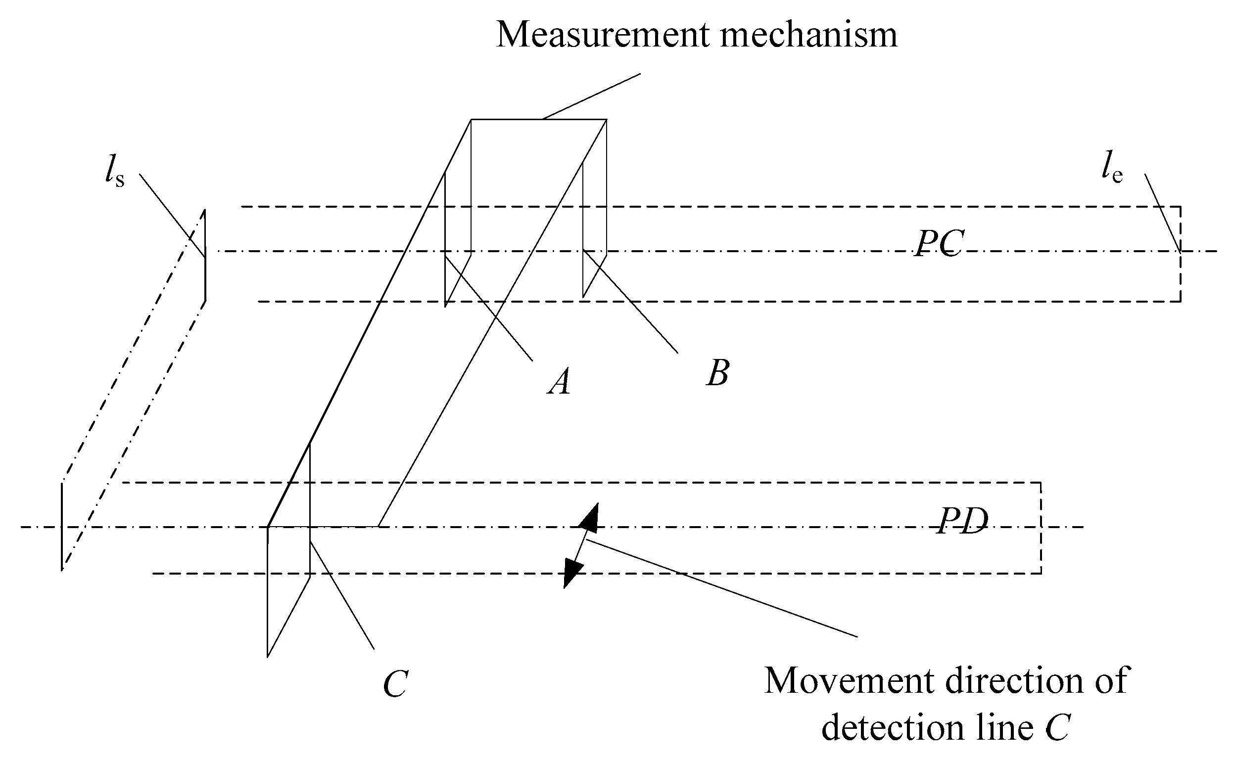
2.2. Measuring Mechanism for Measuring Two Vertical Parallel Surfaces

Figure 5 shows the measuring mechanism for measuring the positional relation of two vertical parallel surfaces. Contact lines A and B are fixed, and the detection line C is movable. The length of contact lines A and B are 70 mm, and detection line C is 50 mm. The contact line A, B, and detection line C are ground after processing, and the processing accuracy grade is IT3.

During the detection process, the fixed contact lines A and B move in one surface, the variable contact line C moves in another detection surface, and the contact lines A, B and the detection line C form a caliper. Under the clamping action of the caliper, the spring generates tension and compression with the shape contour of the measured surface. At the same time, the fluctuate is transmitted to the laser receiving plate along the guide rail, and the laser displacement sensor detects the weak change of the laser receiving plate and records the change through the computer.

As shown in Figure 6a, according to Table 1, start measuring range is 50 mm. When the surface where the contact line A and the detection line C are located are absolutely parallel and the surfaces are absolutely smooth, the detection data is a fixed value and is defined as the initial value X₁. When the shape contours of the two surfaces are considered, the position of the detection line C may change, as shown in Figure 6b. At this time, fluctuating measurements will be generated, and the difference between the measurements and the initial value is the displacement of the detection line C relative to the contact line A.

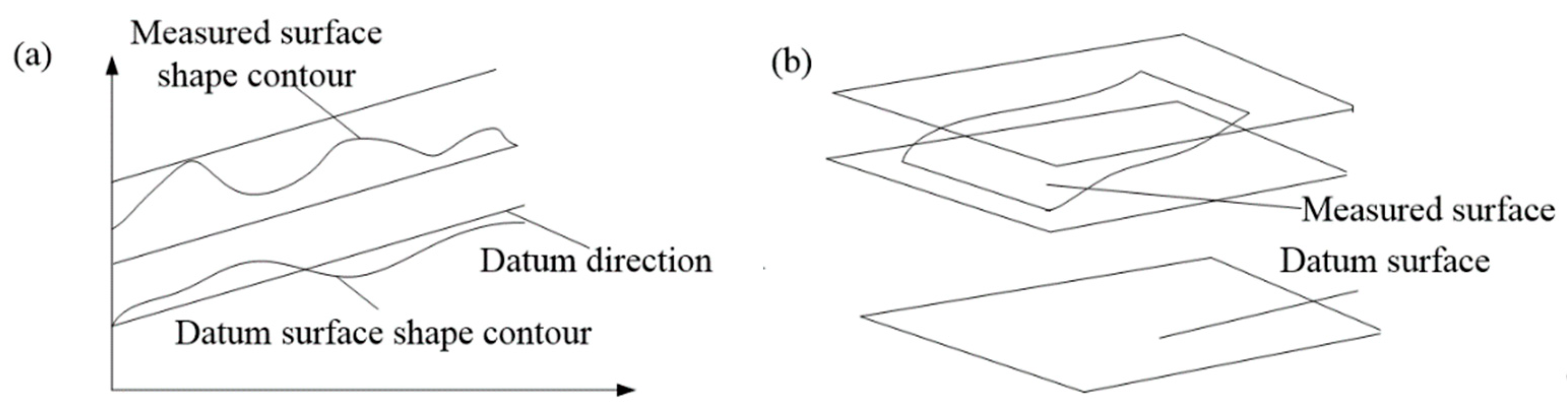
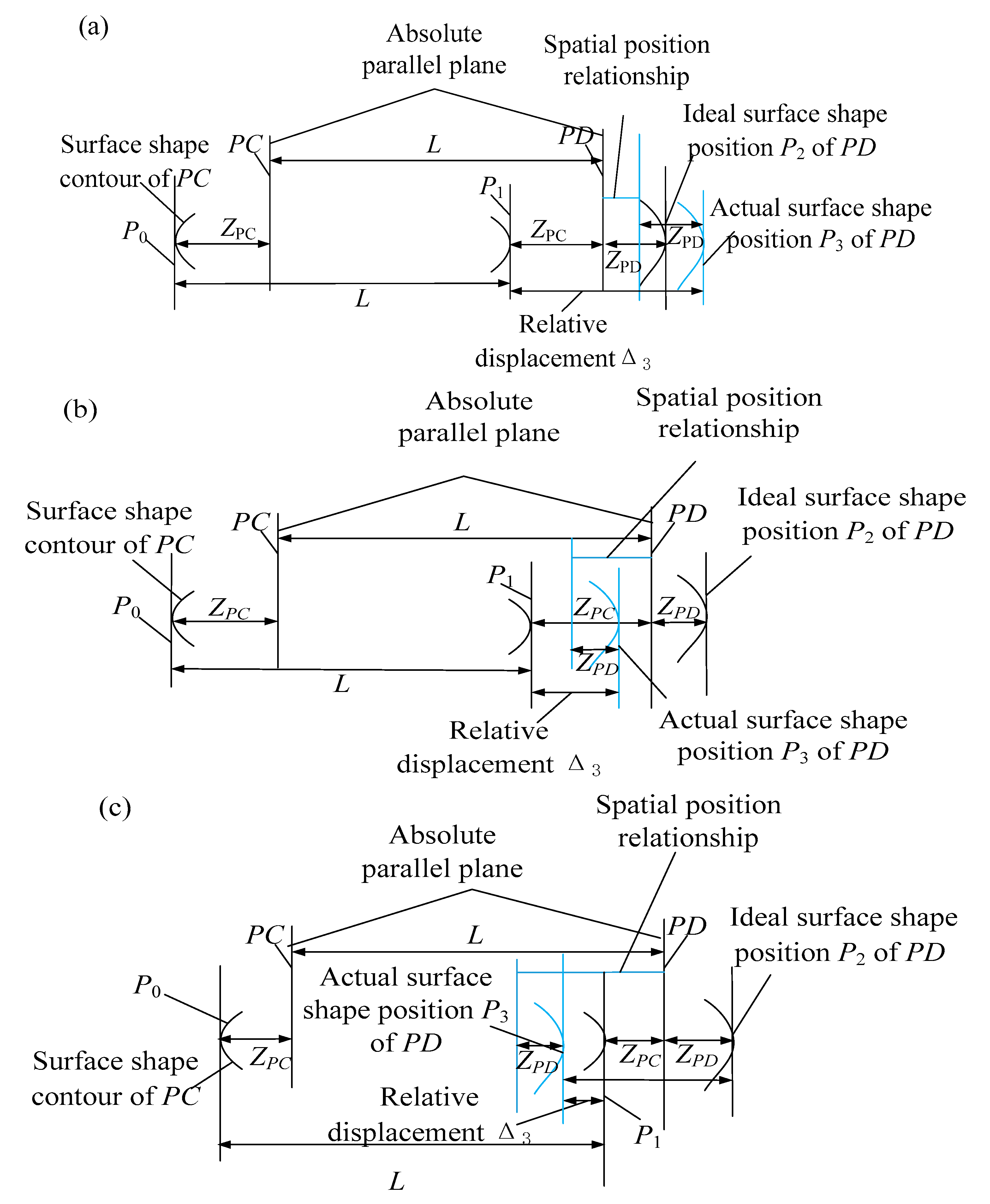
3. The Method for Describing the Positional Relation of Two Parallel Surfaces

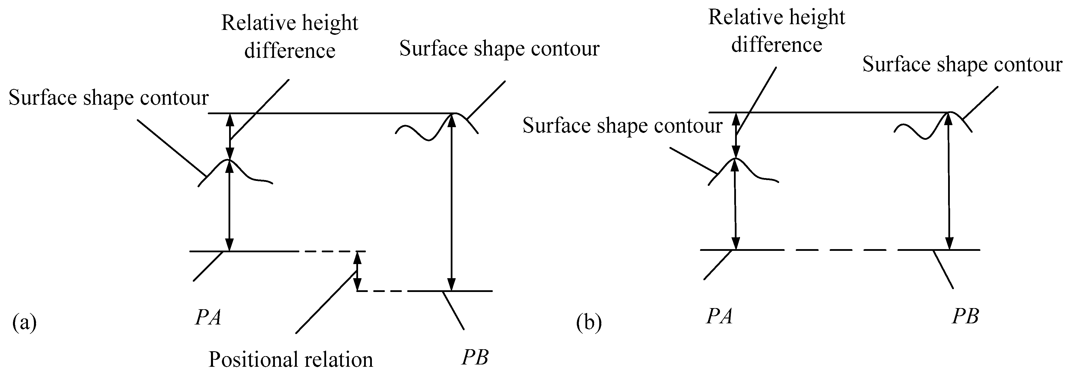
3.1. The Description Method of Positional Relation between Two Horizontal Parallel Surfaces

On the basis of the measurement mechanism in Section 2.1, when A, B, and C are in an absolute smooth surface, the spring is in the initial compression state, this moment, the data recorded by laser displacement sensor is $X_0$, and $X_0$ is defined as the initial value.

Figure 7 shows the measurement model of two horizontal parallel surfaces. With PA as the datum surface, PB as the measured surface. $L_{\mathrm{s}}$ is defined as the starting position, $L_{\mathrm{e}}$ is defined as the terminal position. By coinciding contact line A with $L_{\mathrm{s}}$, the measurement mechanism is driven to move in the direction indicated in Figure 7, and the measurement mechanism is clinging to the auxiliary surface to ensure that there will be no sliding during the measurement process. When contact line A reaches to $L_{\mathrm{e}}$, the measurement is completed, and the data obtained in this process represent effective measurements.

Figure 8a shows the geometric model of PA and PB cross section direction. The shape contour of PB is determined by the shape contour of PA, the relative height difference of PA surface shape contour relative to PB surface shape contour and the positional relation of the two surfaces. According to the mathematical relationship between the effective measurements and $X_0$, the extraction algorithm for combined projection waveform is developed and the combined projection waveform can be obtained. Next, since the measurements of the laser displacement sensor change with time, a time-space conversion algorithm is developed. This algorithm is used to map the time series waveform to the coordinate position of PB surface, which is called the spatial sequence waveform. Then the trend curve of this waveform is found by the method of neural network fitting (a fitting method in the toolbox of MATLAB), which is named as the combined projection curve. This curve is the height difference of PB surface shape contour relative to PA surface shape contour. Due to the shape contour of each surface have been measured before, so they are known quantities. According to the combined projection curve of the PB and the surface shape contour of PA, the separation algorithm for the combined projection curve is studied. The shape contour of PB surface can be obtained by this algorithm, which is called the calculated surface shape contour. When the two surfaces PA and PB are coplanar, as shown in Figure 8b, the positional relation between the two surfaces is zero, and the calculated surface shape contour is the same as the known shape contour of PB surface. If the two results are different, it proves there exists positional relation between two surfaces. Therefore, a description algorithm for positional relation curve between two surfaces is studied. According to the difference between the calculated surface shape contour and the known shape contour of the measured surface, the positional relation between two surfaces can be determined.

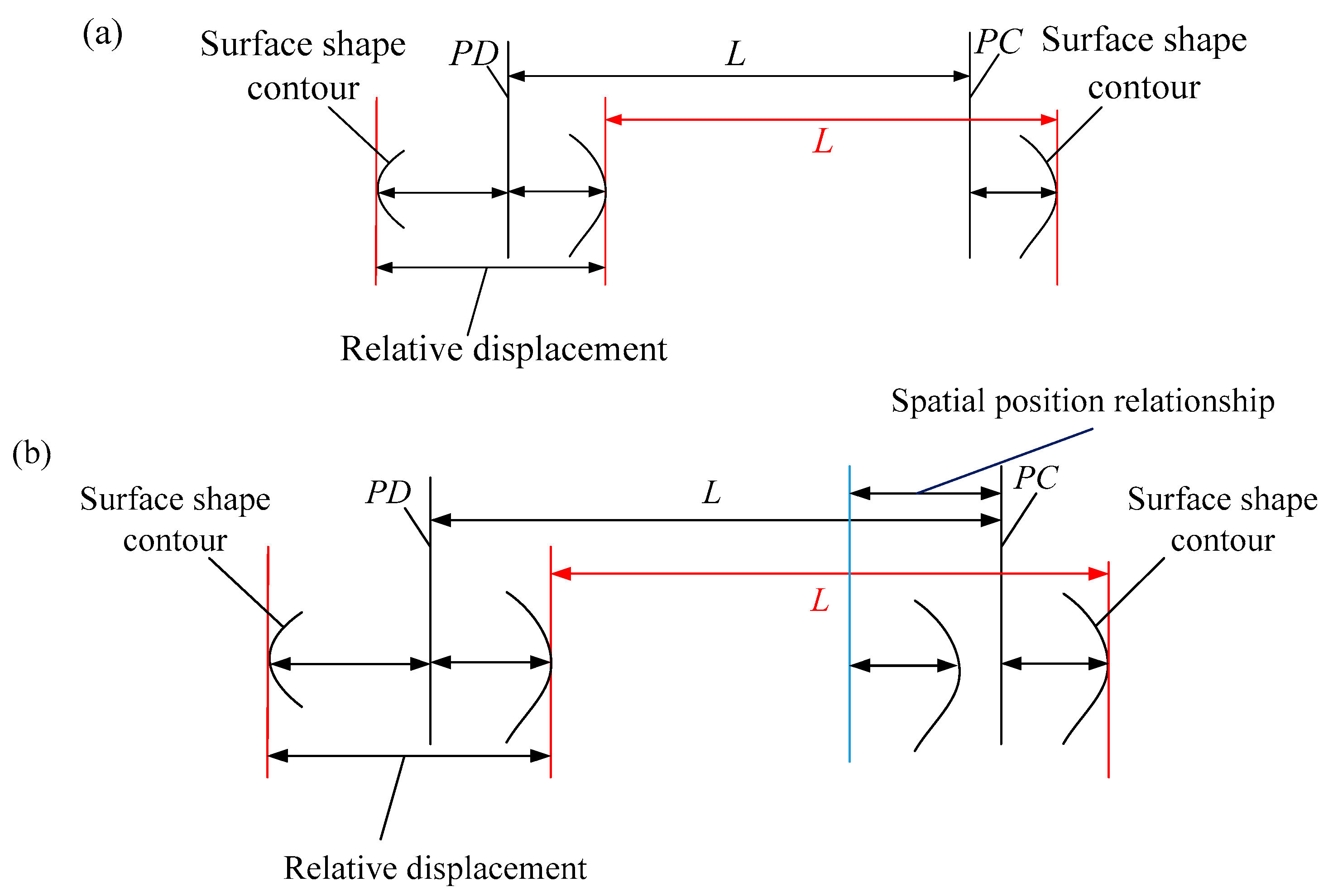
3.2. The Description Method of Positional Relation between Two Vertical Parallel Surfaces

Figure 9 shows the detection model of two vertical parallel surfaces. The detection process and algorithm flow are the same as the detection of two horizontal parallel surfaces

Figure 10 shows the geometric model of PC and PD cross section direction. When PD is the measured surface with PC as the datum surface. If there is no positional relation between the PC and PD surfaces, as shown in Figure 10a. The existed geometric relationship is the surface shape contour and relative displacement of the two surfaces. Since both are known. Therefore, the calculated surface shape contour is the same as the known surface shape contour. If there is an unknown positional relation between the PC and PD surfaces, the relative distance between the shape contours of the two surfaces will change, as shown in Figure 10b. At this time, the shape contour of PD surface cannot be obtained only from the known shape contour of PC surface and relative displacements. Therefore, the calculated shape contour of PD surface is different from the known shape contour of PD surface. Their shape difference is the positional relation curve.

Due to the existing methods can only perform the parallelism evaluation, but the spatial position curve of the two parallel surfaces cannot be depicted. Therefore, it is difficult to carry out a comparative test to verify the test results in this paper.

By definition, parallelism is different to the positional relation of this article. Parallelism requires a datum direction as a datum, which is an orientation error. The positional relation has no datum direction. In this paper, the method of mutual detection by the two surfaces is used to verify the correctness of this detection method. The significance of mutual detection is that, ideally, the positional relation curve obtained by PA, PB mutual detection must be the same shape and opposite direction. The positional relation curve obtained by PC, PD mutual detection must be the same shape. When different measuring mechanisms are used to measure two horizontal parallel surfaces and two vertical parallel surfaces, the same positional relation description method is used to obtain the positional relation curves. However, the datum surface and the measured surface have changed, that is, the movement trajectories of the detection lines A, B, and the contact line C have changed. Under this condition, if the results of the mutual detection are all consistent with the objective law, the correctness of the description method of the positional relation can also be proved.

4. Mathematical Model of the Algorithm

4.1. Mathematical Model for Describing Positional Relation between Two Horizontal Parallel Surfaces

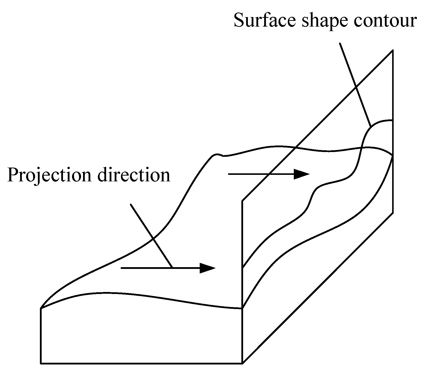
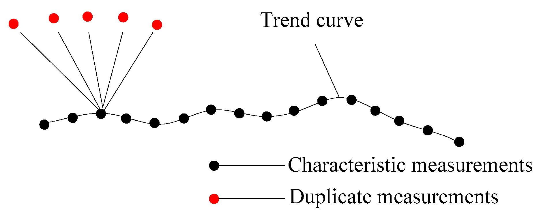
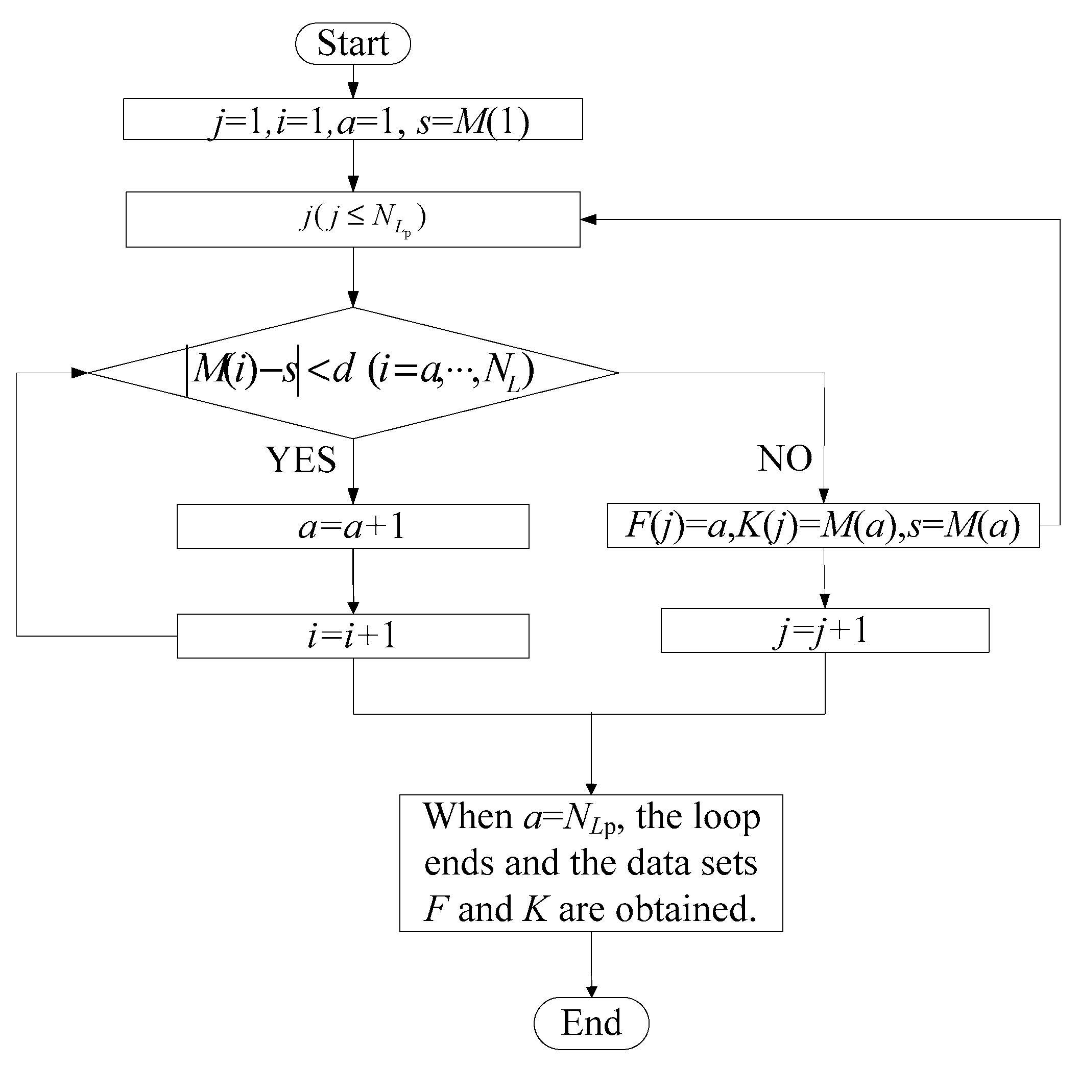
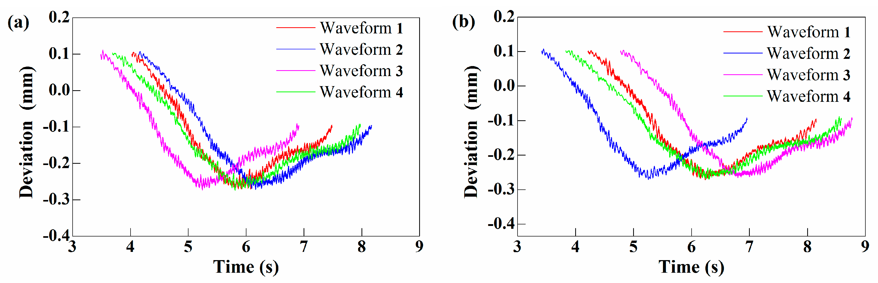
4.1.1. Extraction Algorithm for Combined Projection Waveform

When measuring PB with PA as the datum, the measurements is $X_{\mathrm{s}1}$. When the shape contour of PB surface is higher than PA, the guideway moves upwards, $X_{\mathrm{s}1}<X_0$. When the shape contour of PB surface is lower than PA, the guideway moves downward, $X_{\mathrm{s}1}>X_0$, then the combined projection waveform can be defined as

$$C_1=X_{\mathrm{s}1}-X_0$$

(1)

When measuring PA with PB as the datum, the measurements is $X_{\mathrm{s}2}$, and the moving direction of guideway is opposite to that of measuring PB with PA as datum. When the shape contour of PB surface is higher than PA, the guideway moves downward, $X_{\mathrm{s}2}>X_0$. When the shape contour of PB surface is lower than PA, the guideway moves upwards, $X_{\mathrm{s}2}<X_0$. Then, the combined projection waveform can be defined as

$$C_2=X_{\mathrm{s}2}-X_0$$

(2)

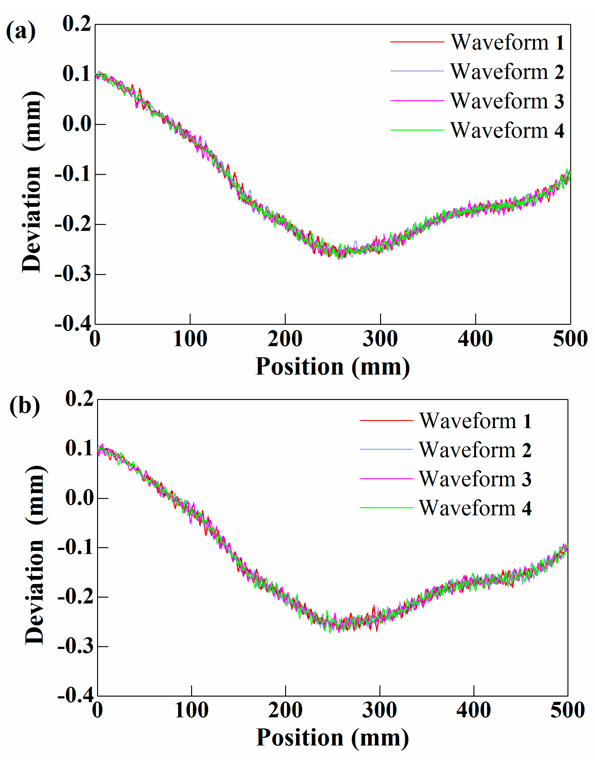
4.1.2. Time-Space Conversion Algorithm

Because the combined projection waveform is time series, it is necessary to converse the measurement waveform of time series into the measurement waveform of spatial sequence. It is known that the sampling frequency of the sensor is as high as 20 kHz, which means that only 0.00005 s is needed to obtain measurement data, indicating that the sampling density is extremely high. At such a high sampling density, the measurements at different times are the same, which means that duplicate measurements are obtained at some detection position, as shown in Figure 11.

Further, due to the high resolution of the sensor, the two adjacent measurements may be at the same position even if the data are not identical. In fact, each detection position only corresponds to one real measurements. Duplicate measurements will interfere with the shape recognition of waveforms. Therefore, the purpose of the time-space conversion algorithm is to extract the measurements at different positions that can recognize the shape of the measurements. These extracted measurements are defined as characteristic measurements.

It is known that sampling frequency and the total number of measurement data, the measurement time t can be expressed as

$$t=\frac{N_{L_{\mathrm{p}}}}{f}$$

(3)

where f is the sampling frequency, $N_{L_{\mathrm{p}}}$ is the total number of sampling data corresponding to the moving distance $L_{\mathrm{p}}$.

Since the speed of the detection mechanism is randomly changed, it is assumed that the average speed of the mechanism travel is 100 mm/s. Taking the sampling interval of the characteristic measurements is 1 mm. At this moment, the time between the two characteristic measurements is 0.01 s. When the velocity between the two characteristic measurements is 50 mm/s and the passing time is 0.01 s, the sampling distance between the two characteristic measurements is 0.5 mm, which is 0.5 mm different from the sampling interval under the average speed, which is insignificant for the overall curve shape of long surface. By extracting the trend curve through the neural network, the effect of the above errors can be eliminated, and only the shape of the whole curve of the waveform can be retained. Therefore, the influence of the driving speed on the detection position can be neglected. Therefore, the average velocity can be selected as the calculation parameter. The average speed of the measurement mechanism is

$$v=\frac{L_{\mathrm{p}}}{t}$$

(4)

where $L_{\mathrm{p}}$ represents the moving distance of the measurement mechanism.

Let M represent the data set of the combined projection waveform. Then, the variables a, j, i, s are created, the initial value of a is 1, $j=1,2,3,\dots ,N_{L_{\mathrm{p}}}$, $i=a,\dots ,N_{L_{\mathrm{p}}}$.

Then, Equation (5) is defined as the objective function.

$$\left|M(i)-s\right|<d$$

(5)

where d is a given value; d is selected according to the actual time series waveform.

If d is too large, the sampling interval of the spatial sequence waveform will be too large, resulting in distortion of the curve shape. If the d is too small, the redundant data cannot be filtered out. M(i) represents the i-th data in the set M. The initial value of s is M(1).

When j = 1, Equation (5) is executed to perform data search, when the searched data meets the objective function condition, a = a + 1, when the condition of the objective function is not met, the data is stored, at this time, the redundant data is filtered out, and the equation can be expressed as follows

$$\{\begin{array}{l}F(j)=a\\ K(j)=M(a)\end{array}$$

(6)

where F(j) represents the position of K(j) in M; K(j) represents the set of characteristic measurements.

Then, perform new calculations on s, and the equation can be expressed as

$$s=M(a)$$

(7)

After Equation (7) is completed, j = j + 1, next, repeat Equations (5)–(7). When $a=N_{L_{\mathrm{p}}}$, the loop is completed. The flow chart of the algorithm is shown in Figure 12.

At this time, the number of data in the sets F and K is $N_{\mathrm{c}}$. It is known that the sampling interval of the measured surface is two characteristic measurements with a certain value difference, so the measurement time between the two characteristic measurements can be expressed as

$$t_{\mathrm{c}}(u)=\frac{F(u)t}{N_{L_{\mathrm{P}}}}$$

(8)

where $F(u)$ represents the u-th data in set F, u = 1, 2, 3, …, N_c;

The measurement waveform of spatial sequence corresponding to the coordinate position on the measured surface can be obtained according to Equation (9), so the time-space conversion of the data can be realized and Equation (9) can be expressed as follows

$$\begin{array}{ll}v{t}_{\mathrm{c}}(1)& \stackrel{}{\to }K(1)\\ v{t}_{\mathrm{c}}(2)& \stackrel{}{\to }K(2)\\ \cdot & \cdot \\ \cdot & \cdot \\ \cdot & \cdot \\ v{t}_{\mathrm{c}}(N_{\mathrm{c}})& \stackrel{}{\to }K(N_{\mathrm{c}})\end{array}$$

(9)

where t_c(1, …, N_c) is derived from Equation (8); K(1, …, N_c) is derived from Equation (6).

At this time, the spatial sequence waveform corresponding to the combined projection waveform C₁ can be represented by R₁, and the spatial sequence waveform corresponding to the combined projection waveform C₂ can be represented by R₂. After that, the trend curves Δ₁ and Δ₂ of R₁ and R₂ are extracted respectively, and Δ₁ is defined as the combined projection curve of R₁, Δ₂ is defined as the combined projection curve of R₂.

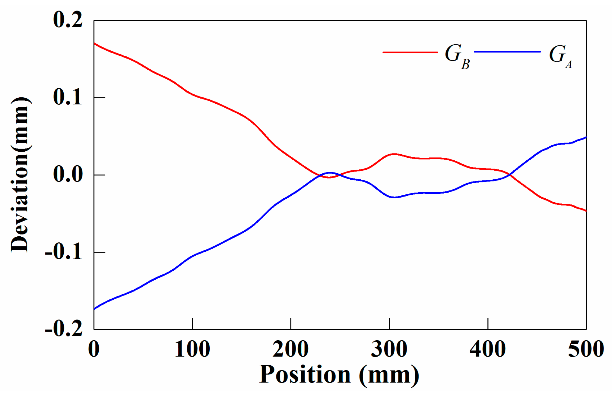
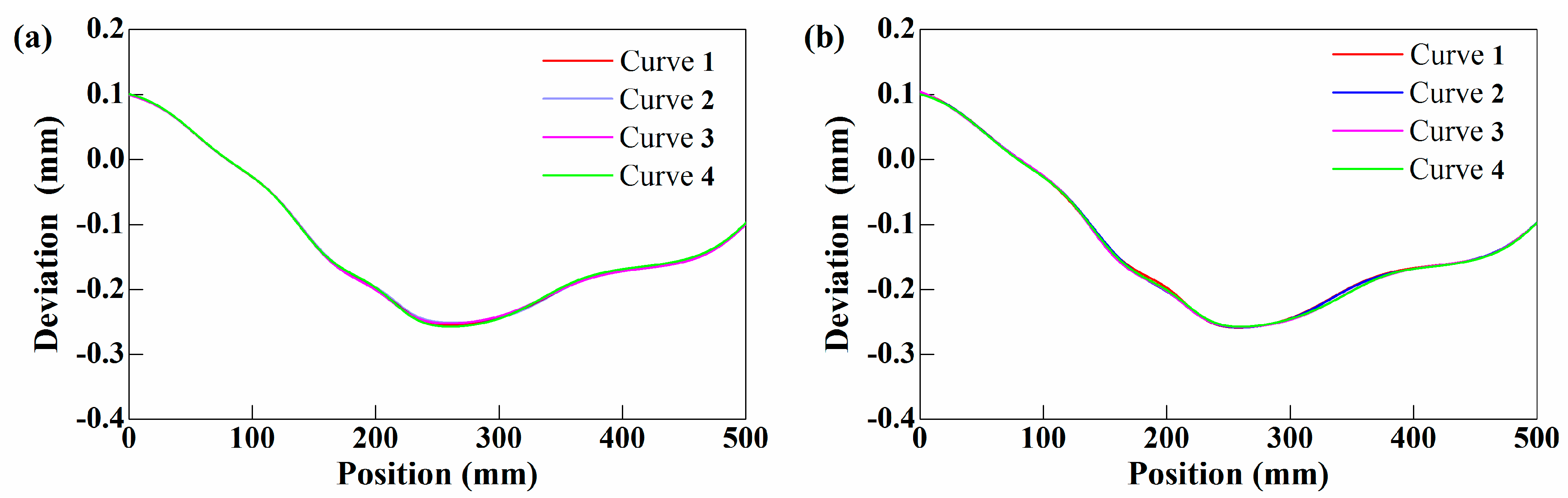
4.1.3. Separation Algorithm for Combined Projection Curve

The separation algorithm model of the combined projection curve is shown in Figure 13.

With PA as the datum surface and PB as the measured surface, the calculated shape contour can be defined as

$$S_{\mathrm{PB}}=Z_{\mathrm{PA}}\pm \left|{\Delta }_1\right|$$

(10)

where Z_PA is the shape contour of PA surface, when Δ₁ < 0, uses ‘+’, when Δ₁ > 0, uses ‘−’.

With PB as the datum surface and PA as the measured surface, the calculated shape contour can be defined as

$$S_{\mathrm{PA}}=Z_{\mathrm{PB}}\pm \left|{\Delta }_2\right|$$

(11)

where Z_PB is the shape contour of PB surface, when Δ₂ < 0, uses ‘+’, when Δ₂ > 0, uses ‘−’.

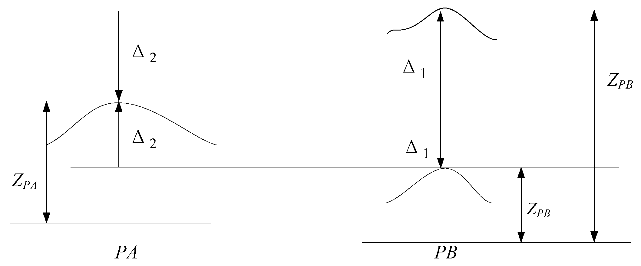
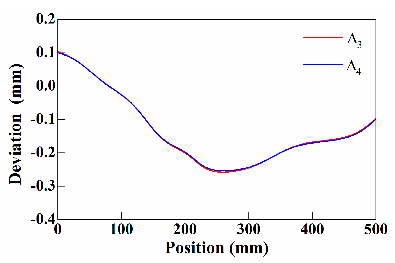
4.1.4. Description Algorithm for Positional Relation

When PB is the measured surface, PA as the datum, the positional relation curve of PB relative to PA can be expressed as

$$G_{\mathrm{B}}=S_{\mathrm{PB}}-Z_{\mathrm{PB}}$$

(12)

where Z_PB is the shape contour of PB surface.

When PA is the measured surface, PB as the datum, the positional relation curve of PA relative to PB can be expressed as

$$G_{\mathrm{A}}=S_{\mathrm{PA}}-Z_{\mathrm{PA}}$$

(13)

where Z_PA is the shape contour of PA surface.

4.2. Mathematical Model for Describing Positional Relation between Two Vertical Parallel Surfaces

4.2.1. Extraction Algorithm for Combined Projection Waveform

Three kinds of situations may occur during the measurement of two vertical parallel surfaces. As the detection model shown in Figure 14, when PD is measured surface with the PC as the datum surface, the measurements is $X_{\mathrm{s}3}$. When the contact line A is at $P_0$ and the detection line C is at $P_1$, the distance between the surface where the contact line A is located and the surface where the detection line C is located is the same as the distance between the two surfaces which are absolutely parallel, and both are L. At this time, the measurement is fixed, defined as $X_1$. Ideally, in the case where there is no positional relation between the two surfaces, the detection line C should be located at $P_2$, and the contact line A should be located at $P_0$. Since two absolutely parallel surfaces do not exist, the actual detection line C should be located at $P_3$.

In the detection model shown in Figure 14a,b, the spring is in compression state, at this time, X_s3 < X₁. In the detection model shown in Figure 14c, the spring is in the stretching state, at this time, X_s3 > X₁. Then, the combined projection waveform can be defined as

$$C_3=X_{\mathrm{s}3}-X_1$$

(14)

When measuring PC with PD as datum, the measurement is $X_{\mathrm{s}4}$, when the spring is in compression state, $X_{\mathrm{s}4}<X_1$, and when the spring is in stretching state, $X_{\mathrm{s}4}>X_1$. Then, the combined projection waveform can be defined as

$$C_4=X_{\mathrm{s}4}-X_1$$

(15)

At this time, the spatial sequence waveform corresponding to the combined projection waveform C₃ can be represented by R₃, and the spatial sequence waveform corresponding to the combined projection waveform C₄ can be represented by R₄. After that, the trend curves Δ₃ and Δ₄ of R₃ and R₄ are extracted respectively, and Δ₃ is defined as the combined projection curve of R₃, while Δ₄ is defined as the combined projection curve of R₄.

4.2.2. Separation Algorithm for Combined Projection Curve

The separation algorithm model of the combined projection curve is shown in Figure 14. With PC as the datum surface, PD as the measured surface, the calculated shape contour can be defined as

$$S_{\mathrm{PD}}=-{\Delta }_3-Z_{\mathrm{PC}}$$

(16)

where Z_PC is the shape contour of PC surface.

With PD as the datum surface, PC as the measured surface, the calculated shape contour can be defined as

$$S_{\mathrm{PC}}=-{\Delta }_4-Z_{\mathrm{PD}}$$

(17)

where Z_PD is the shape contour of PD surface.

4.2.3. Description Algorithm for Positional Relation

When PC is the measured surface, PD as the datum, the positional relation curve of PD relative to PC can be expressed as

$$G_{\mathrm{D}}=S_{\mathrm{PD}}-Z_{\mathrm{PD}}$$

(18)

When PC is the measured surface, PD as the datum, the positional relation curve of PD relative to PC can be expressed as

$$G_{\mathrm{C}}=S_{\mathrm{PC}}-Z_{\mathrm{PC}}$$

(19)

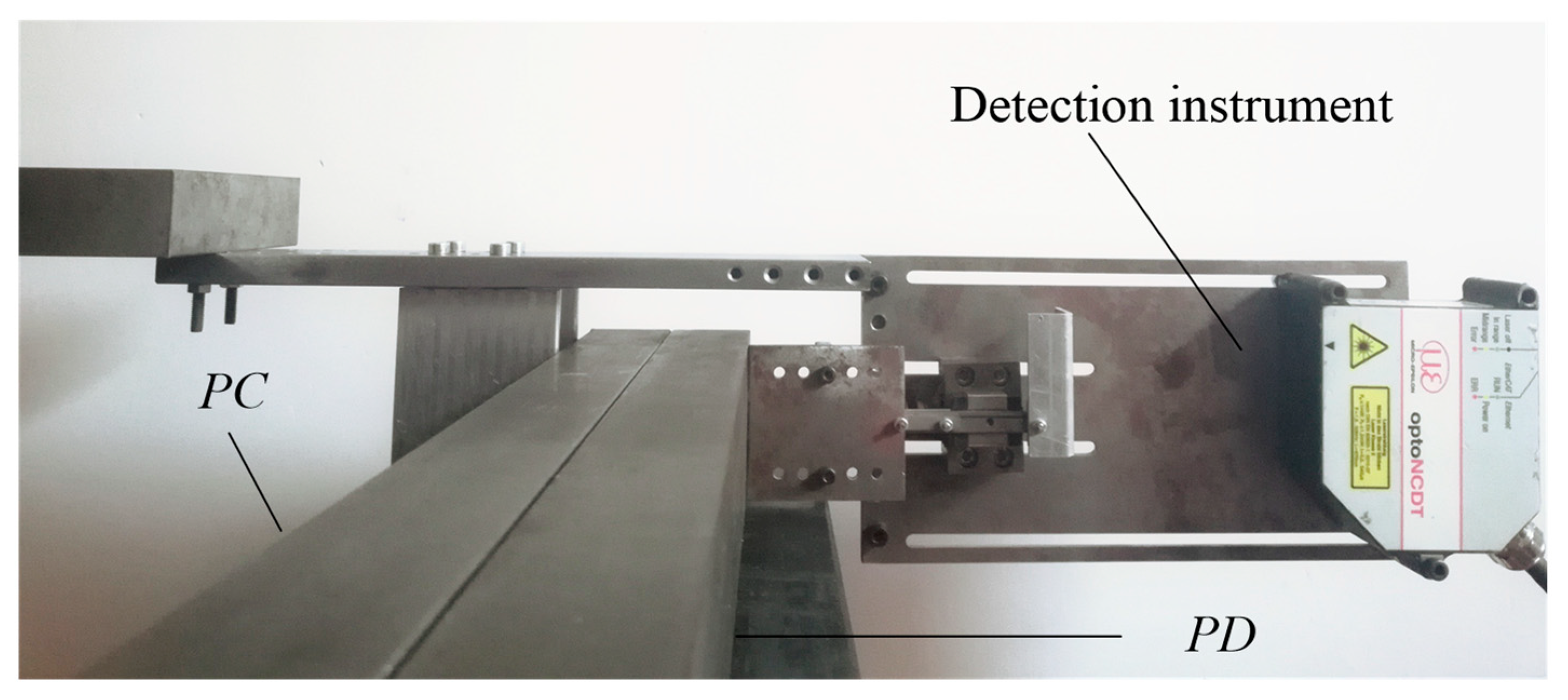
5. Experimental Validation

5.1. Measuremen Texperiment of Two Horizontal Parallel Surfaces

5.1.1. Experimental Step

In order to verify the correctness of this measurement method, the measurement experiment was carried out. Before measuring, a marble flat ruler with class 000 precision as shown in Figure 2 was selected as the datum surface, the size of the marble flat ruler selected in this paper is 500 × 100 × 50 mm, and its flatness is 1.5μm. Therefore, it can be regarded as an approximately absolute horizontal plane. Then, the measurement mechanism was placed on the surface of marble ruler to calibrate the initial value $X_0$. It is assumed that contact line A and detection line C are on the same horizontal surface. Place the detection mechanism at different positions on the marble flat ruler and find the average of the five measurements, then the initial value $X_0$ can be obtained, and $X_0$ is 32.92014 mm.

Taking PA and PB surfaces with a length of 500 mm and a width of 50 mm, the distance between the two surfaces is 60 mm. Calibrating the starting and ending positions, ensure that the spring is in compression. Firstly, the PB surface was detected by using PA surface as the datum surface, as shown in Figure 15a, and then the PA surface was detected by using PB surface as the datum surface, as shown in Figure 15b. The measurement method is described in Section 3.1. Each surface was measured four times. During the measurement process, the measurement mechanism moves along the auxiliary surface toward the arrow direction. Under the constraint of an auxiliary surface, the detection mechanism will not slide.

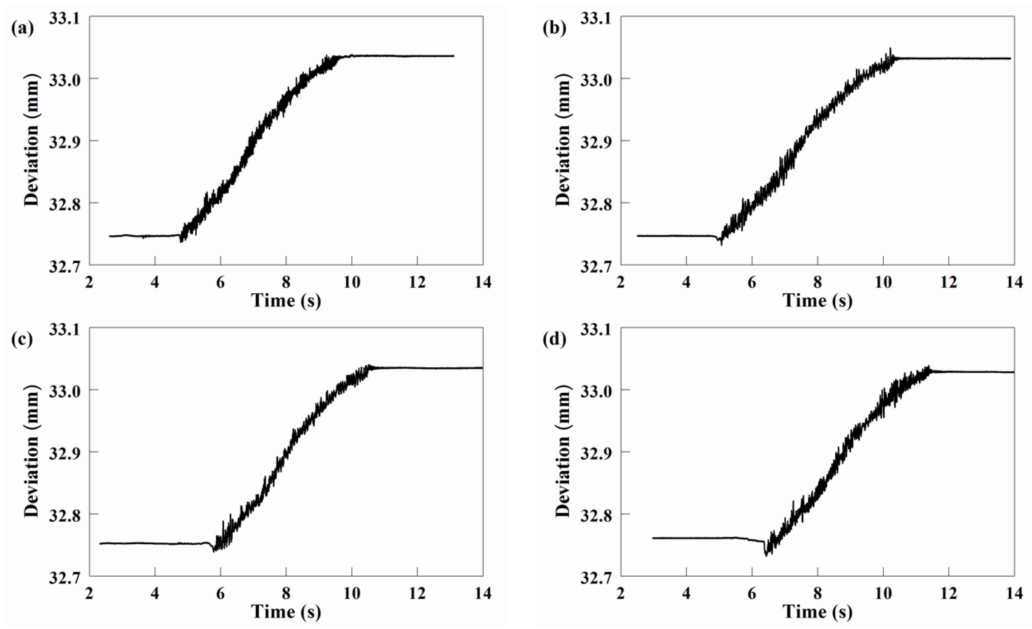
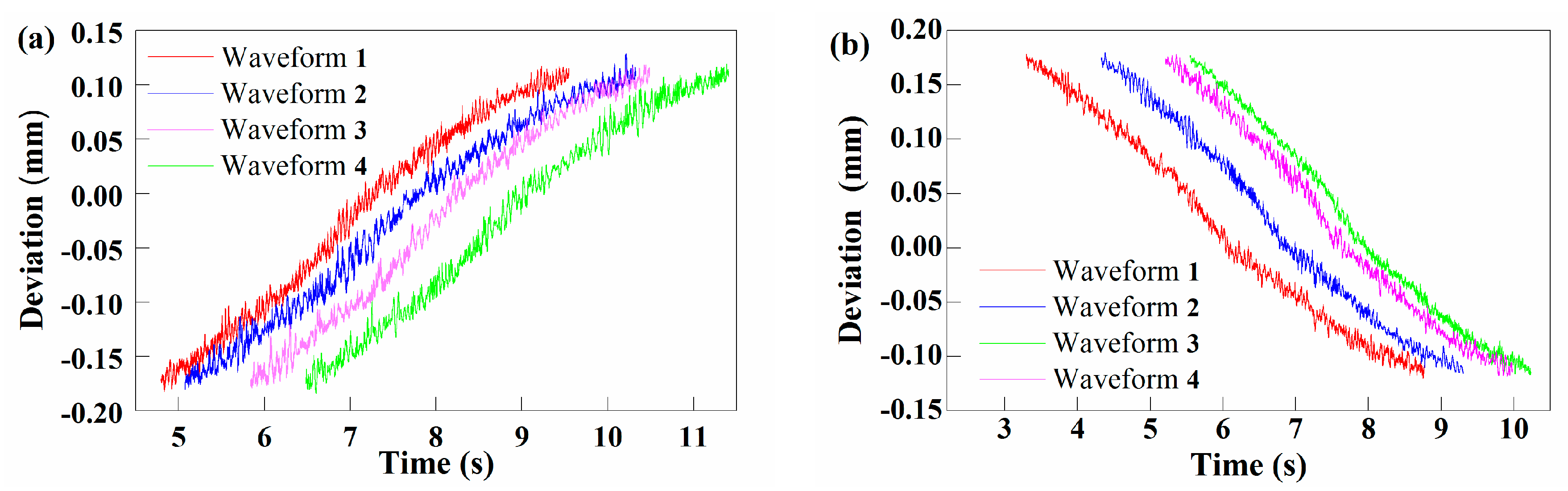
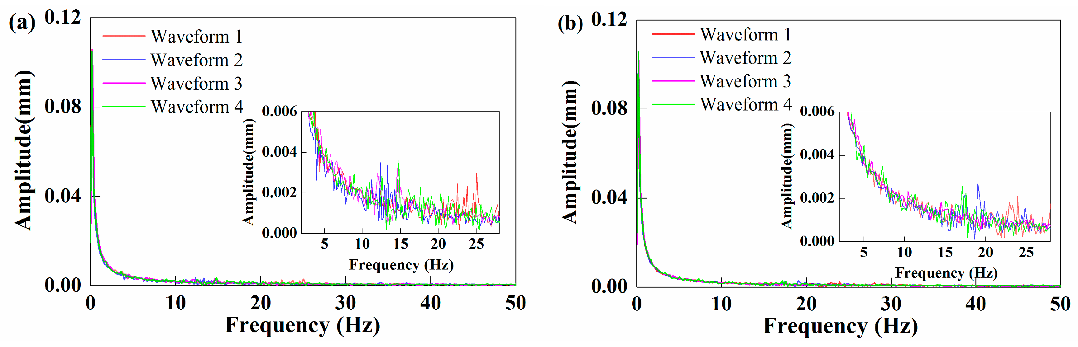
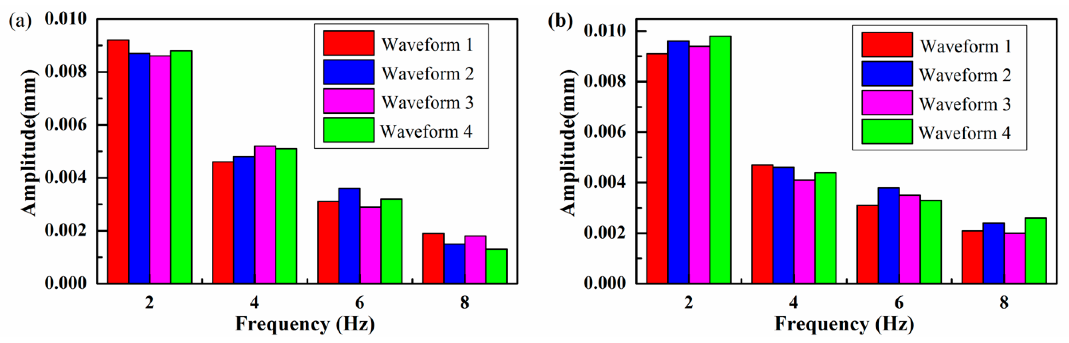
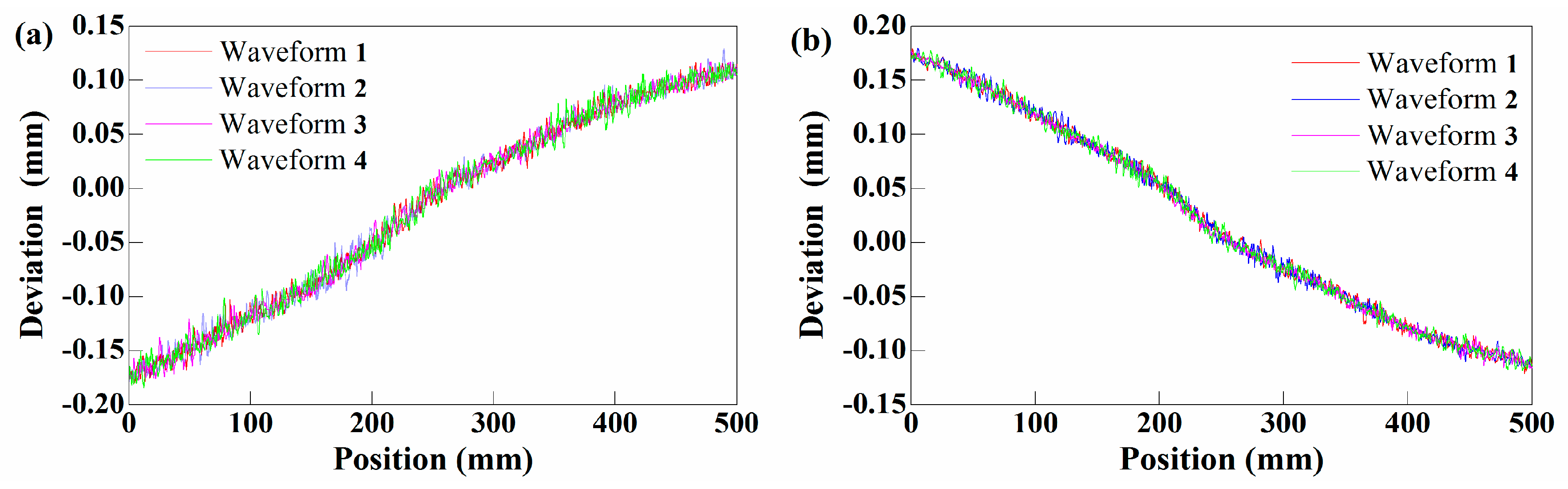
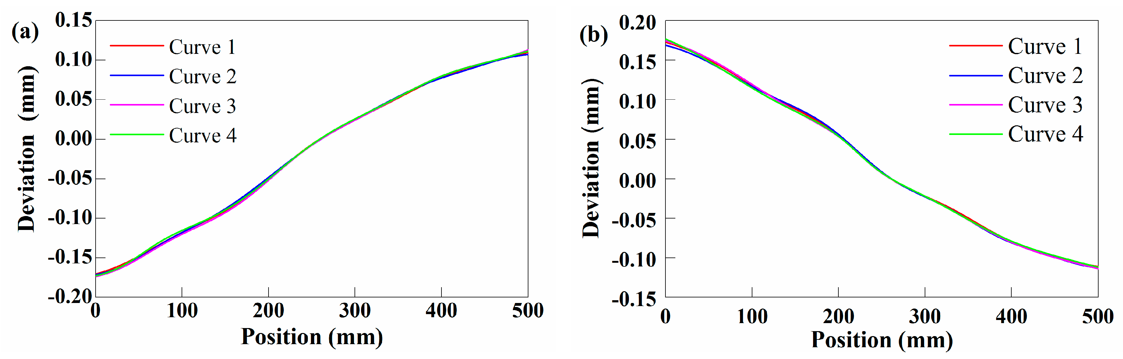
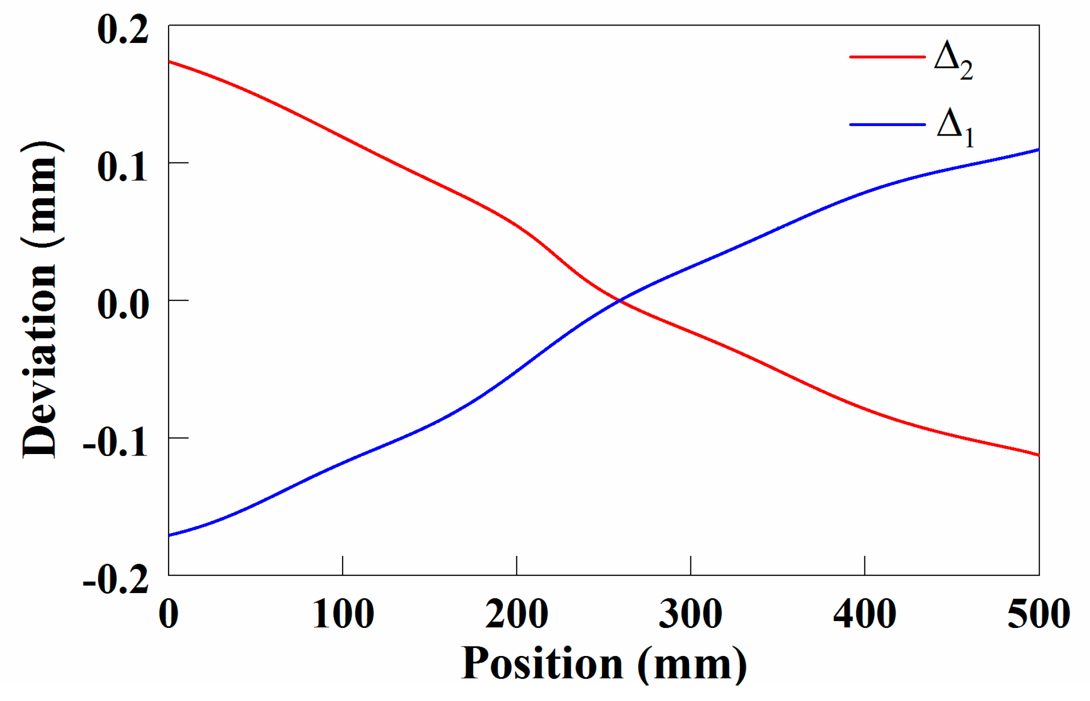
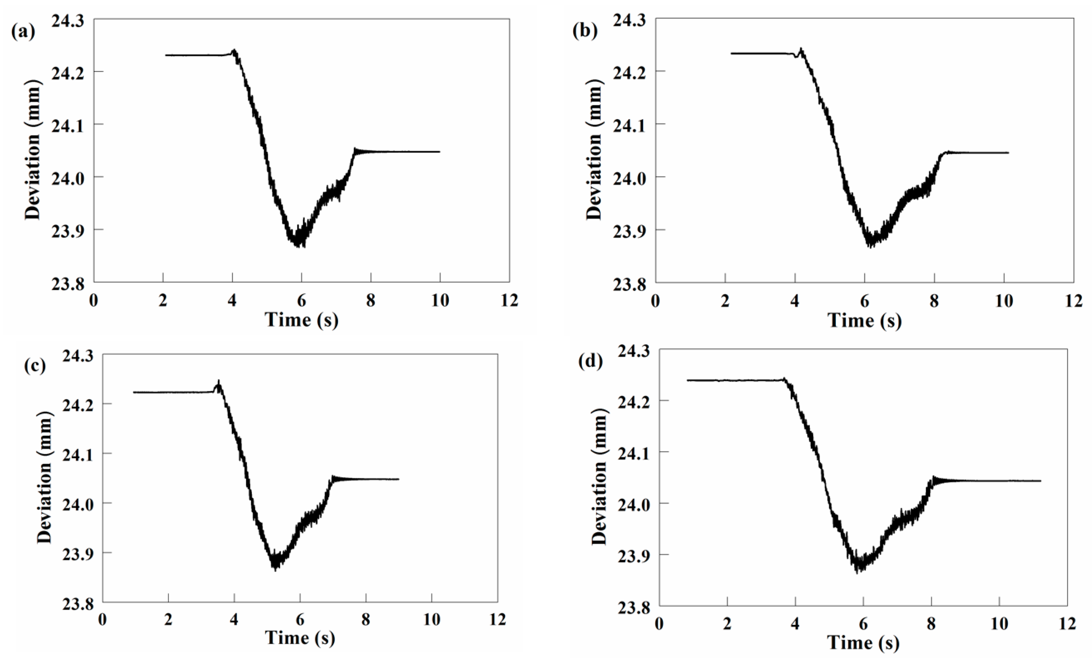
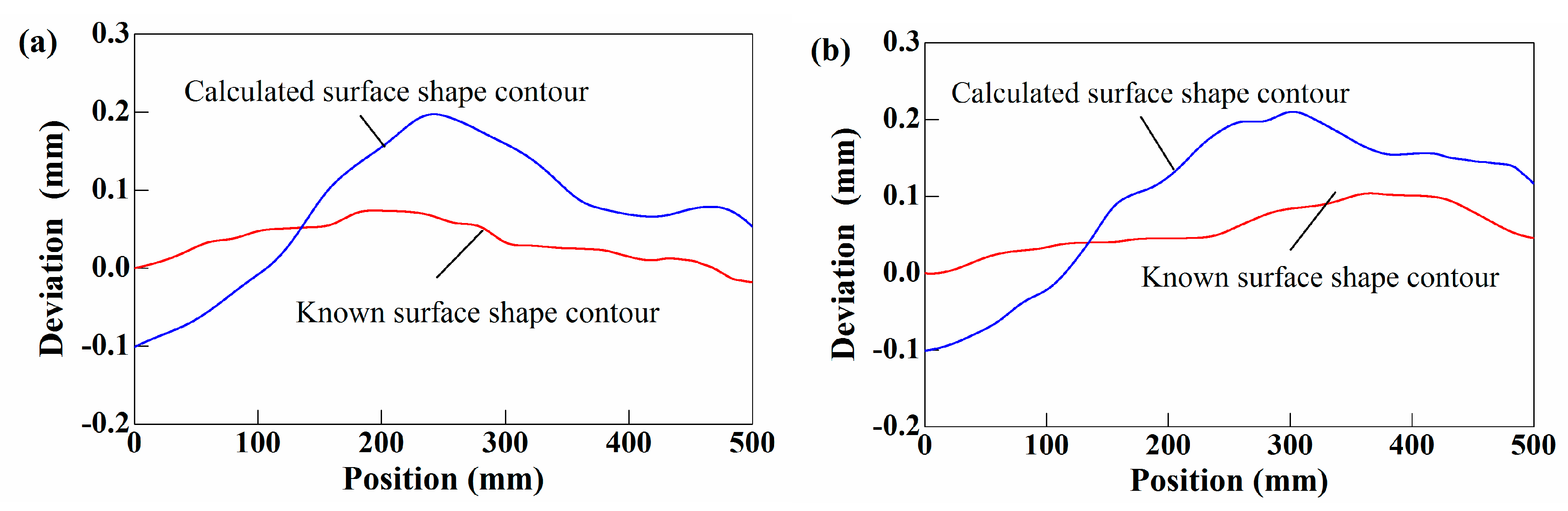
5.1.2. Results and Analysis

The measurements of laser displacement sensor are shown in Figure 16 and Figure 17. When the contact line A is located at the starting position, computer begins to record the data. After the contact line A reached the end position, where it necessary to save the data, the measurement mechanism is in a static state, and the measurements of this process represent a straight line approaching the level. It is known that the measurements between starting position and end position is defined as valid measurements. Therefore, the suspended time series waveforms need to be separated and the effective measurements were obtained.

When the effective measurements and $X_0$ were obtained, the combined projection waveforms were calculated according to Equations (1) and (2). Figure 18 shows the combined projection waveforms. It can be seen that the waveforms change with sampling time, and the measurement time is different, which has greater randomness.

The measurements in Figure 18 are sequenced according to the measurement time from short to long. Then, FFT is carried out to obtain the amplitude frequency characteristics, as shown in Figure 19. It can be seen from the analysis of the amplitude of the low-frequency band that the amplitudes of the spectrum graphs corresponding to different waveforms are basically identical. Further, the peak mainly occurs near 0 Hz and there is no frequency doubling relationship in the amplitude frequency characteristics. This is because the measurements changes with the shape of the measured plane and is not affected by other factors. When 2–28 Hz is amplified, it is found that the amplitude does not increase or decrease monotonously with the increase of measurement time. It shows that the measurement time has no effect on the amplitude frequency characteristics of the measurements. It can also be understood that when four waveforms are converted into spatial sequences, the overall shape of the waveforms does not change significantly.

Extracting the amplitude corresponding to the 2 Hz, 4 Hz, 6 Hz, 8 Hz, as shown in Figure 20, it can be seen that the amplitude corresponding to the same frequency has little difference with varying measurement time, indicating that different driving speed has little impact on the attribute of measurements. Therefore, the average velocity can be used as the calculation parameter.

Then the waveforms in Figure 18 are processed by the time-space conversion algorithm. The converted spatial sequence waveforms are shown in Figure 21. Because the positional relation curve is macro geometric, therefore, the trend curves of the waveforms in Figure 21 are extracted, which are called the combined projection curves, as shown in Figure 22. It can be seen from Figure 21 and Figure 22, when the measurement mechanism detects the identical surface, A, B, and C always pass the shape contours of the identical surfaces. Although the characteristic measurements at the same position are not exactly the same, but the overall shape of the waveform trend curve is constant, the combined projection curves on the identical measured surfaces are close to coincidence. This shows that the detection mechanism has good repeatability and stability, and the time–space conversion algorithm successfully converts the waveforms of time–deviation into the position–deviation.

Figure 23 shows the average of combined projection curve of the PA and PB surfaces. Here, the data structure is the same as that of the known surface shape contours in Figure 24, and each datum corresponds to the identical detection position. As can be seen from Figure 23 the combined projection curves obtained by mutual measurement of the two surfaces are symmetrically distributed with 0 as the center, which accords with the mathematical relationship of the data corresponding to the same position in the two surfaces in Figure 13.

Based on the above analysis, substituting the data in Figure 23 and Figure 24 into Equations (10) and (11), the calculated surface shape contours are obtained, as shown in Figure 25. It can be seen from Figure 25 that the calculated surface shape contours are different from the known surface shape contours, which indicates that there exists a positional relation between two surfaces PA and PB.

Finally, the data in Figure 25 were substituted into Equations (12) and (13) to obtain the difference curve between the calculated surface shape contour and the known surface shape contour, as shown in Figure 26. The curve describes the positional relation of the two surfaces. It can be seen from Figure 26. The positional relation curve obtained by mutual check has the same shape and symmetric distribution, which is consistent with the principle of a positional relation between two horizontal parallel planes. The maximum error is 4.07 μm, which has little effect on the overall shape of the curve. The correctness of this detection method can be proved.

5.2. Measuremen Texperiment of Two Vertical Parallel Surfaces

5.2.1. Experimental Step

In order to verify the correctness of the algorithm for describing the positional relation between two vertical parallel surfaces, a measurement experiment was performed using a homemade measuring instrument, and the measurement site is shown in Figure 27. Before measurement, choosing a class 000 marble ruler with length of 100 mm, width of 60 mm, and height of 50 mm. As its parallelism is 1μm, the surfaces on both sides of the marble ruler can be approximately regarded as absolutely smooth parallel surfaces. Firstly, place the contact lines A, B, and the detection line C on both sides of the marble ruler, and tightly clamp the marble ruler. Then, the initial value $X_1$ can be obtained and $X_1$ is 24.1379 mm.

The method for detecting the positional relation between two vertical parallel surfaces is the same as the method for detecting the positional relationship between two horizontal surfaces. Firstly, use the PC as the datum surface to detect the PD surface, and then use the PD surface as the datum surface to detect the PC surface. Repeat the measurement four times for each surface.

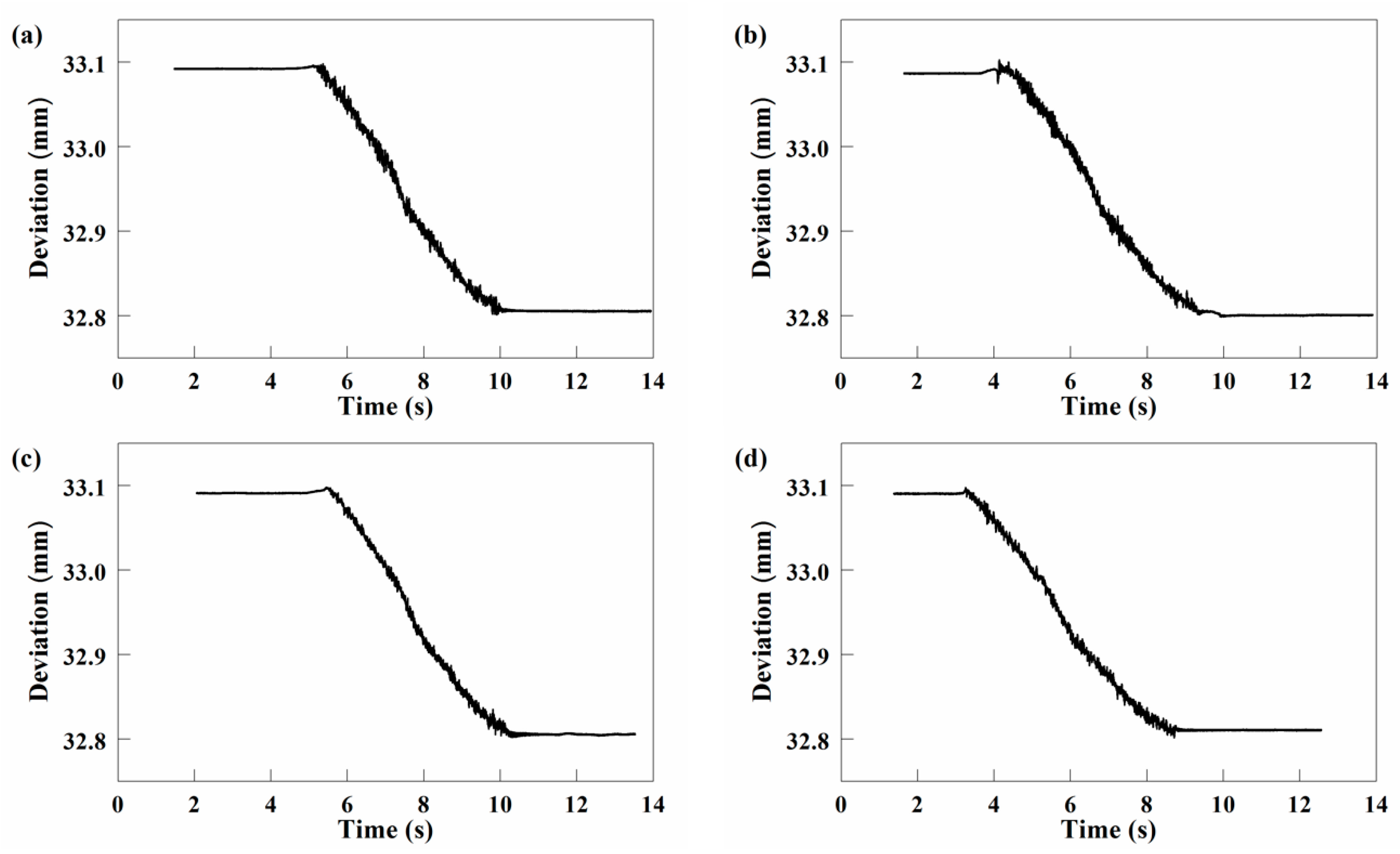
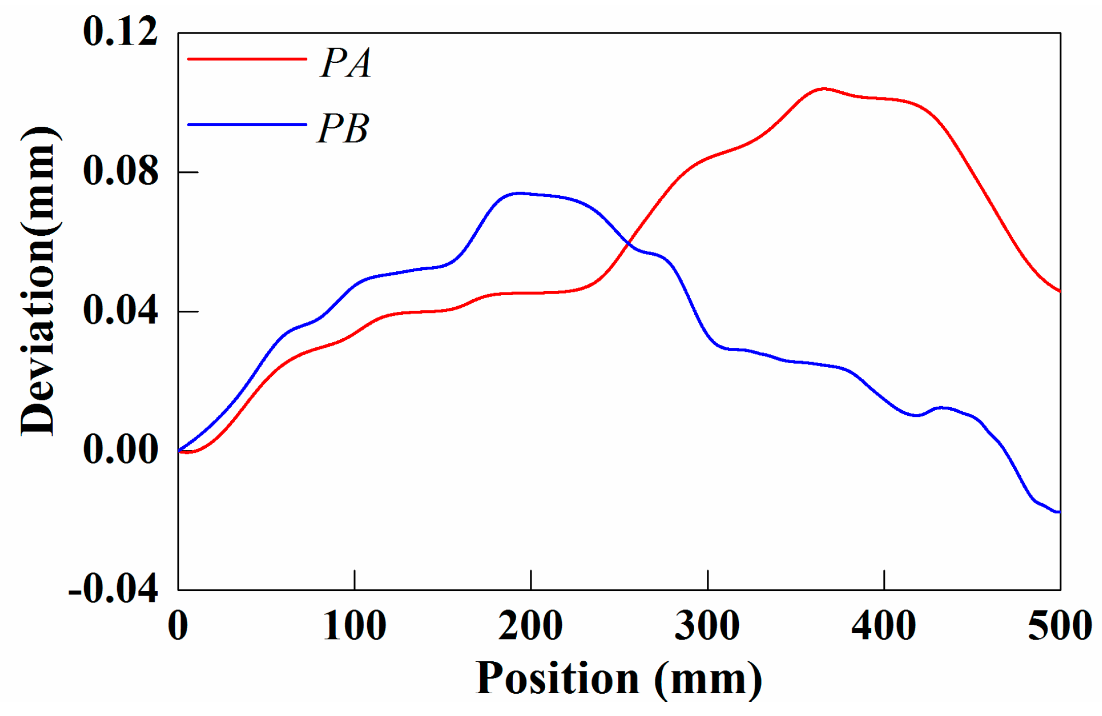
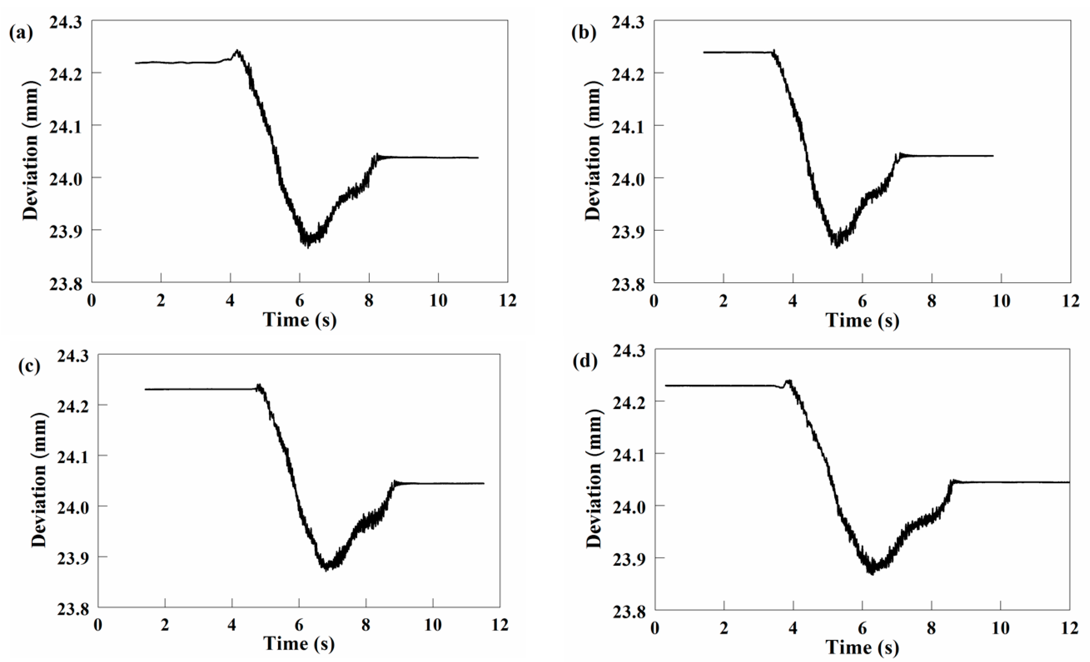
5.2.2. Results and Analysis

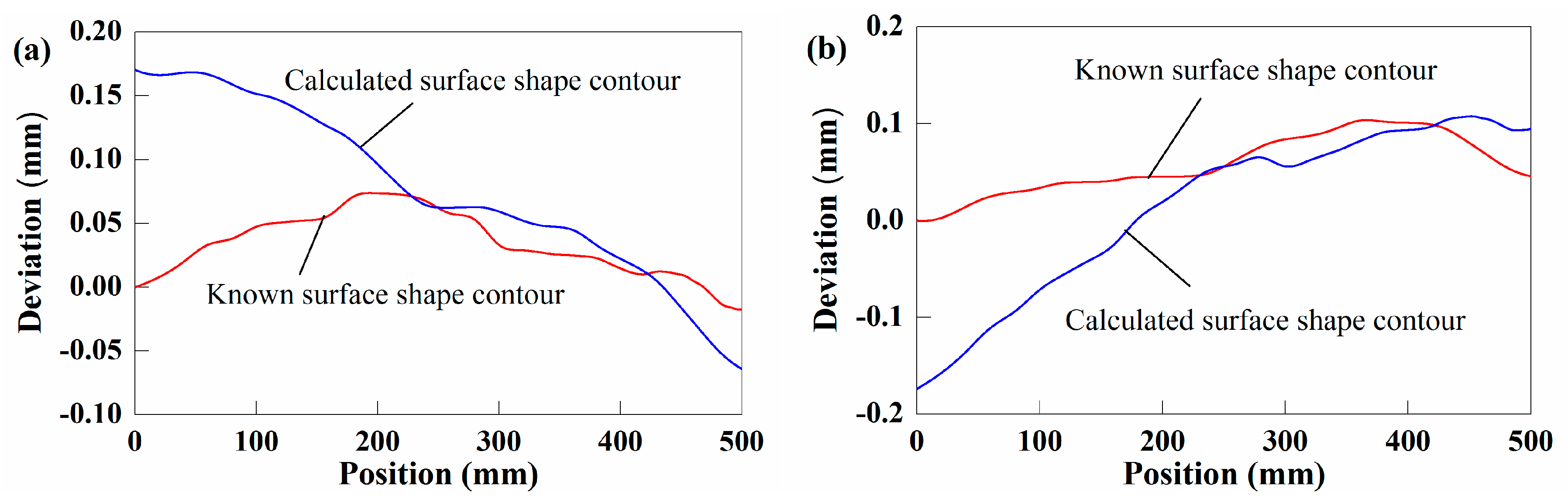
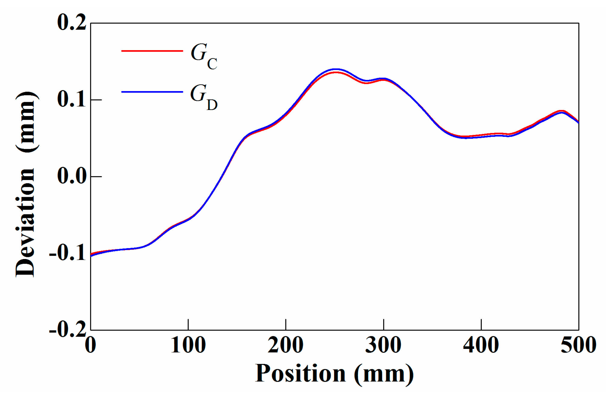
The original measurement data recorded by the computer is shown in Figure 28 and Figure 29. When the contact line A is located at the starting position, computer begins to record the data. After the contact line A reached the end position, where it is also necessary to save the data, the measurement mechanism is in a static state, and the measurement of this process is a straight line approaching the level. It is known that the measurement between starting position and end position is defined as a valid measurement. Therefore, the suspended time series waveforms need to be separated and the effective measurements were obtained.

Extract the effective measurements, according to Equations (14) and (15), and the combined projection waveform will be obtained, as shown in Figure 30.

It can be seen from the Figure 19 and Figure 20 that the measurement time has no effect on the overall shape of the waveforms. Then, use the space-time conversion algorithm to obtain the spatial sequence waveform, as shown in Figure 31. The trend curve of the waveform in Figure 31 is extracted to obtain a combined projection curve, as shown in Figure 32. The projection curves obtained from multiple measurement are close to coincidence, which shows that the detection mechanism also has high repeatability and stability when applied to the detection of vertical surface, which proves the rationality of the design of the detection mechanism in the vertical direction.

Figure 33 shows the average of the combined projection curve of PC and PD surfaces. It can be seen from Figure 33 that the combined projection curves are close to coincide. It is proved that the relative displacement of the two vertical surfaces is only related to the distance of the detection line C relative to the datum surface, independent of the direction, and in line with the geometric relationship in the detection model in Figure 14.

Based on the above analysis, the data in Figure 24 and Figure 33 are substituted into Formulas (16) and (17) to obtain the calculated surface shape contours, as shown in Figure 34. It can be seen from Figure 34 that the calculated surface shape contour is different from the known surface shape contour, indicating that there exists a positional relation between the two surfaces.

Finally, the data in Figure 34 are substituted into Equations (18) and (19) to obtain the difference curve between the calculated surface shape contour and the known surface shape contour, as shown in Figure 35. The curve describes the spatial relationship between PC and PD surfaces. As can be seen from Figure 35, the shape of positional relation curves obtained by mutual detection are close to coincidence, which id consistent with the principle of positional relation between two vertical parallel surfaces. The maximum error of the two positional relation curves is 4.56 μm, which has little effect on the overall shape of the curve. The correctness of this detection method can be proved.

5.3. Discussion

In order to verify whether this method is correct and whether the detection instruments are designed reasonably, only short span tests are carried out in this paper. When measuring the two surfaces with large span, as long as the detection mechanisms are in a balanced state, there will be no sliding. Therefore, this method can still be used for measurement of large span surfaces.

Because the contact lines A, B, and detection line C have shape errors, and the combined projection waveform is equal to the measurements minus the initial value, therefore the influence of the shape errors of the contact lines A, B, and detection line C on the measurement results can be eliminated.

During the detection progress, the measurements will be affected by motion error, surface roughness, spring damping and other factors. However, the influence of these factors accounts for a small proportion of the measurements. Since the position relation curve is macro, the trend curve reflects the overall shape of the measurements. The extracted trend curve has a certain inclusiveness to the peak and valley of the waveform. When the trend curve of the waveform is extracted, the error components in the measurements will be largely separated. Therefore, the error has little effect on the shape of trend curve and the error of the final positional relation curve mainly comes from the method of extracting the trend curve.

The article focuses on verifying the correctness of the detection method and whether the detection mechanism can be applied to actual measurement. The next work will focus on the analysis of the uncertainty of detection methods and the detection process.

6. Conclusions

This paper proposed a method for describing the positional relation of two parallel surfaces on-site. The extraction algorithm for combined projection waveform, time-space conversion algorithm, the separation algorithm for combined projection curve, and the description algorithm for positional relation are successfully developed. It can be seen from the experimental results that the combined projection curves obtained by detecting the same surface are nearly coincident, indicating that the detection mechanism has high repeatability. The extracted trend curve has a certain inclusiveness to the peak and valley of the waveform. Although the measurements affected by motion error, surface roughness, spring damping, and others factor, the error has little effect on the shape of trend curve. The results of the mutual detection of the two examples are in accordance with the objective law. The maximum error of the positional relation curve obtained by the mutual detection of the two horizontal parallel surfaces is 4.07 μm, and the maximum error of the position relation curve obtained by the mutual detection of the two vertical parallel surfaces is 4.56 μm, which has little effect on the curve shape, indicating that this method can accurately obtain the positional relation between two horizontal parallel planes and two vertical parallel planes. The measurement mechanisms are designed reasonably, and the measurement method is correct. It is operable in practical application.

Moreover, it can be completed in two minutes from the acquisition of the detection data to the drawing of the positional relation curve of two surfaces, which means high efficiency. Compared with the existing parallelism evaluation method, the positional relation curve obtained by this method makes the description of the position error of two parallel planes more specific. Compared with the existing measurement instruments, the mechanisms are more suitable for field measurement of large equipment. This research demonstrates innovation, and it is also of great significance to the requirements of modern industries such as field measurement and the digitalization of assembly processes.

References

1. Zha, J.; Xue, F.; Chen, Y. Straightness error modeling and compensation for gantry type open hydrostatic guideways in grinding machine. Int. J. Mach. Tools Manuf. 2017, 112, 1–6. [Google Scholar] [CrossRef]
2. Kang, C.S.; Kim, J.A.; Jin, J. An optical straightness measurement sensor for the KRISS watt balance. Measurement 2015, 61, 257–262. [Google Scholar] [CrossRef]
3. Borisov, O.; Fletcher, S.; Longstaff, A. New low cost sensing head and taut wire method for automated straightness measurement of machine tool axes. Opt. Lasers Eng. 2013, 51, 978–985. [Google Scholar] [CrossRef] [Green Version]
4. Wei, X.; Su, Z.; Yang, X.; Lv, Z.; Yang, Z.; Zhang, H.; Li, X.; Fang, F. A Novel Method for the Measurement of Geometric Errors in the Linear Motion of CNC Machine Tools. Appl. Sci. 2019, 9, 3357. [Google Scholar] [CrossRef] [Green Version]
5. Li, P.; Ding, X.M.; Tan, J.B. A hybrid method based on reduced constraint region and convex-hull edge for surface evaluation. Precis. Eng. 2016, 45, 168–175. [Google Scholar] [CrossRef]
6. Radlovački, V.; Hadžistević, M.; Štrbac, B. Evaluating minimum zone surface using new method—Bundle of plains through one point. Precis. Eng. 2016, 43, 554–562. [Google Scholar] [CrossRef]
7. Giusca, C.L.; Claverley, J.D.; Sun, W. Practical estimation of measurement noise and flatness deviation on focus variation microscopes. CIRP Ann. Manuf. Technol. 2014, 63, 545–548. [Google Scholar] [CrossRef]
8. Han, Z.; Chen, L.; Wulan, T. The absolute flatness measurements of two aluminum coated mirrors based on the skip flat test. Opt. Int. J. Light Electron Opt. 2013, 124, 3781–3785. [Google Scholar] [CrossRef]
9. Haijun, L.; Zhigang, D.; Han, H. A new method for measuring the flatness of large and thin silicon substrates using a liquid immersion technique. Meas. Sci. Technol. 2015, 26, 115008. [Google Scholar]
10. Zhou, P.; Xu, K.; Wang, D. Rail Profile Measurement Based on Line-structured Light Vision. IEEE Access 2018, 6, 16423–16431. [Google Scholar] [CrossRef]
11. Srinivasu, D.S.; Venkaiah, N. Minimum zone evaluation of roundness using hybrid global search approach. Int. J. Adv. Manuf. Technol. 2017, 92, 2743–2754. [Google Scholar] [CrossRef]
12. Cao, Z.; Wu, Y.; Han, J. Roundness deviation evaluation method based on statistical analysis of local least square circles. Meas. Sci. Technol. 2017, 28, 105017. [Google Scholar]
13. Hsieh, T.H.; Huang, H.L.; Jywe, W.Y. Development of a machine for automatically measuring static/dynamic running parallelism in linear guideways. Rev. Sci. Instrum. 2014, 85, 035115. [Google Scholar] [CrossRef] [PubMed]
14. Hwang, J.; Park, C.H.; Gao, W. A three-probe system for measuring the parallelism and straightness of a pair of rails for ultra-precision guideways. Int. J. Mach. Tools Manuf. 2017, 47, 1053–1058. [Google Scholar] [CrossRef]
15. Bhattacharya, J.C. Measurement of parallelism of the surfaces of a transparent sample. Opt. Lasers Eng. 2001, 35, 27–31. [Google Scholar] [CrossRef]
16. Lee, K.I.; Shin, D.H.; Yang, S.H. Parallelism error measurement for the spindle axis of machine tools by two circular tests with different tool lengths. Int. J. Adv. Manuf. Technol. 2017, 88, 2883–2887. [Google Scholar] [CrossRef]
17. Vannoni, M.; Bertozzi, R. Parallelism error characterization with mechanical and interferometric methods. Opt. Lasers Eng. 2007, 45, 719–722. [Google Scholar] [CrossRef]
18. Jywe, W.Y.; Hsieh, T.H.; Chen, P.Y.; Wang, M.S. An Online Simultaneous Measurement of the Dual-Axis Straightness Error for Machine Tools. Appl. Sci. 2018, 8, 2130. [Google Scholar] [CrossRef] [Green Version]
19. Hsieh, T.H.; Chen, P.Y.; Jywe, W.Y.; Chen, G.W.; Wang, M.S. A Geometric Error Measurement System for Linear Guideway Assembly and Calibration. Appl. Sci. 2019, 9, 574. [Google Scholar] [CrossRef] [Green Version]
Figure 1. Evaluation method of parallelism: (a). Line-to-line (b). Surface to surface.
Applsci 10 02152 g001
Figure 2. Measurement mechanism for measuring two horizontal parallel surfaces.
Applsci 10 02152 g002
Figure 3. Detection path.
Applsci 10 02152 g003
Figure 4. The positional relation between contact line A and detection line C: (a). Contact line A and detection line C are collinear; (b). Contact line A and detection line C are not collinear.
Applsci 10 02152 g004
Figure 5. Measuring mechanism for measuring two vertical parallel surfaces.
Applsci 10 02152 g005
Figure 6. The positional relation between contact line A and detection line C: (a) The distance between the contact line A and the detection line C is unchanged (b) Contact line A and detection line C are located in two surfaces with shape contours.
Applsci 10 02152 g006
Figure 7. Detection model of two horizontal parallel surfaces.
Applsci 10 02152 g007
Figure 8. Geometric model of PA and PB cross section direction: (a) Positional relation exists between PA and PB surfaces. (b)Positional relation does not exists between PA and PB surfaces.
Applsci 10 02152 g008
Figure 9. Detection model of two vertical parallel surfaces.
Applsci 10 02152 g009
Figure 10. Geometric model of PC and PD cross section direction: (a) Positional relation does not exists between PC and PD surfaces. (b)Positional relation exists between PC and PD surfaces.
Applsci 10 02152 g010
Figure 11. Structure of measurements.
Applsci 10 02152 g011
Figure 12. Flow chart of the algorithm.
Applsci 10 02152 g012
Figure 13. Separation algorithm model of the combined projection curve.
Applsci 10 02152 g013
Figure 14. Separation algorithm model of the combined projection curve: (a) Model 1; (b) Model 2; (c) Model 3.
Applsci 10 02152 g014
Figure 15. Measurement system of two horizontal parallel surfaces. (a) PB is the measured surface. (b) PA is the measured surface.
Applsci 10 02152 g015
Figure 16. The measurements when PB is the measured surface (a) measurements 1 (b) measurements 2 (c) measurements 3 (d) measurements 4.
Applsci 10 02152 g016
Figure 17. The measurements when PA is the measured surface (a) measurements 1 (b) measurements 2 (c) measurements 3 (d) measurements 4.
Applsci 10 02152 g017
Figure 18. Combined projection waveforms. (a) PB is the measured surface (b) PA is the measured surface.
Applsci 10 02152 g018
Figure 19. Amplitude frequency characteristics of measurements. (a) PB is the measured plane (b) PA is the measured plane.
Applsci 10 02152 g019
Figure 20. Amplitude corresponding to frequency 2 Hz, 4 Hz, 6 Hz, 8 Hz. (a) PB is the measured plane (b) PA is the measured plane.
Applsci 10 02152 g020
Figure 21. Combined projection waveforms of spatial sequence (a) PB is the measured surface. (b) PA is the measured surface.
Applsci 10 02152 g021
Figure 22. Combined projection curves. (a) PB is the measured surface. (b) PA is the measured surface.
Applsci 10 02152 g022
Figure 23. The average of the combined projection curves of the PA and PB surfaces.
Applsci 10 02152 g023
Figure 24. Known surface shape contours.
Applsci 10 02152 g024
Figure 25. Comparison between the calculated surface shape contour and known surface shape contour: (a) PB is the measured surface. (b) PA is the measured surface.
Applsci 10 02152 g025
Figure 26. Two positional relation curves.
Applsci 10 02152 g026
Figure 27. Measurement system of two vertical parallel surfaces.
Applsci 10 02152 g027
Figure 28. The measurements when PD is the measured surface (a) measurements 1 (b) measurements 2 (c) measurements 3 (d) measurements 4.
Applsci 10 02152 g028
Figure 29. The measurements when PC is the measured surface (a) measurements 1 (b) measurements 2 (c) measurements 3 (d) measurements 4.
Applsci 10 02152 g029
Figure 30. Combined projection waveforms: (a) PD is the measured surface (b) PC is the measured surface.
Applsci 10 02152 g030
Figure 31. Combined projection waveforms of spatial sequence: (a) PD is the measured surface (b) PC is the measured surface.
Applsci 10 02152 g031
Figure 32. Combined projection curves (a) PD is the measured surface (b) PC is the measured surface.
Applsci 10 02152 g032
Figure 33. The average of the combined projection curves of the PC and PD surfaces.
Applsci 10 02152 g033
Figure 34. Comparison between calculated surface shape contour and known surface shape contour: (a) PD is the measured surface (b) PC is the measured surface.
Applsci 10 02152 g034
Figure 35. Two positional relation curves.
Applsci 10 02152 g035