Nonlinear Model and Dynamic Behavior of Photovoltaic Grid-Connected Inverter

Abstract

A photovoltaic grid-connected inverter is a strongly nonlinear system. A model predictive control method can improve control accuracy and dynamic performance. Methods to accurately model and optimize control parameters are key to ensuring the stable operation of a photovoltaic grid-connected inverter. Based on the nonlinear characteristics of photovoltaic arrays and switching devices, we established a nonlinear model of photovoltaic grid-connected inverters using the state space method and solved its model predictive controller. Then, using the phase diagram, folded diagram, and bifurcation diagram methods, we studied the nonlinear dynamic behavior under the influence of control parameters on both fast and slow scales. Finally, we investigated the methods of parameter selection based on the characteristics of nonlinear dynamic behavior. Our research shows that the predictive controller parameters are closely related to the bifurcation and chaos behaviors of the grid-connected photovoltaic inverter. The three-dimensional bifurcation diagram can be used to observe the periodic motion region of the control parameters. After selecting the optimization target, the bifurcation diagram can be used to guide the selection of control parameters for inverter design. The research results can be used to guide the modeling, stability analysis, and optimization design of photovoltaic grid-connected inverters.

1. Introduction

In recent years, with the development of new energy generation technologies, more and more photovoltaic grid-connected inverters are being connected to the power grid, making the modeling and stability of new power grids a hot research subject [1,2,3]. Converting a photovoltaic array into an equivalent variable voltage source greatly simplifies the modeling, control strategy, and stability analysis of photovoltaic grid-connected inverters [4] and especially reduces the computation costs for small-world network models [5]. Similarly, by simplifying the H-bridge switch circuit appropriately and then establishing an equivalent model, the analysis, controller design, and numerical simulation of multi-paralleled grid-connected inverters are greatly simplified [6]. A photovoltaic array is a typical nonlinear device that may have a great impact on the accuracy of a photovoltaic grid-connected inverter model after simplification. With the rapid increase in the computing capabilities of modern microprocessors, researchers are increasingly exploring nonlinear models to improve the accuracy of system models. Nonlinear models of photovoltaic arrays can allow for analysis of the nonlinear characteristics of the system, thus providing more accurate modeling for photovoltaic grid-connected inverter [7,8,9].

An inverter circuit contains power switching devices, which are strongly nonlinear systems. Establishing a piecewise smooth model can better reveal the inherent physical characteristics of the system, such as bifurcation and chaos [10,11,12,13]. Since the 1980s, the nonlinear dynamic behaviors of power electronics systems have been widely studied, including the bifurcation and chaotic behaviors of DC/DC converters [14,15,16], DC/AC converters [11,13,17], and motor systems [18,19]. Studies have shown that the bifurcation and chaotic behaviors are closely related to the control and stability of power electronic systems, the bifurcation behavior of multi-inverter microgrids has an inherent relationship with system stability [20,21], and chaos control in power electronics systems is crucial for system stability [22,23]. With the continuous increase of the number of distributed photovoltaic grid-connected inverters, accurate system modeling, control, and stability analysis are becoming more and more important. Only by comprehensively considering the nonlinear characteristics of photovoltaic arrays and the switching characteristics of inverter circuits can accurate models of photovoltaic grid-connected inverters be established.

The main work of this paper is to establish a nonlinear model for photovoltaic grid-connected inverters and solve its predictive controller, study the nonlinear dynamic behavior of photovoltaic grid-connected inverters using methods including time-domain waveforms, phase diagrams, folded diagrams, and bifurcation diagrams, and finally explore how to select control parameters using nonlinear dynamic behavior characteristics such as bifurcation and chaos. The work of this paper may serve as a valuable reference in the modeling, optimization control, and stability analysis of large-scale distributed new energy grid-connected power generation systems.

2. Circuit Structure and Operational Principle of Photovoltaic Grid-Connected Inverter

A single-phase full-bridge photovoltaic (PV) grid-connected inverter is a typical circuit structure of photovoltaic grid-connected inverters. In single-phase PV grid-connected inverter, there are two typical structures, namely single-stage structure, and two-stage structure. The two-stage structure is to add a DC/DC converter in front of the DC/AC converter, which enables MPPT (Maximum Power Point Tracking) to be carried out in the DC/DC converter. For a single-stage structure, MPPT is placed in DC/AC. From the control point of view, the two-stage structure can be separated from the grid-connected control and MPPT control, which is more convenient for control, but low conversion efficiency. In the single-stage structure, the grid-connected control and MPPT control are integrated. Although the control is relatively complex, it can be easily realized at present. The single-stage structure is relatively simple, which helps improve efficiency. To express this more simply, in this paper, we use a single-stage structure for analysis.

The circuit, as shown in Figure 1, consists of a power block, an isolation block, and a control block. In the power block, the PV array and the capacitor ${\mathrm{C}}_1$ constitute the power input source; ${\mathrm{M}}_1–{\mathrm{M}}_4$ constitute the full-bridge circuit; ${\mathrm{L}}_1$, ${\mathrm{L}}_2$, and ${\mathrm{C}}_2$ constitute the LCL output filter; $R_{\mathrm{L}}$ is the equivalent resistance of the circuit conductor wires; and $u_{\mathrm{g}}$ is the signal of the public power grid. In Figure 1, $i_{\mathrm{PV}}$ and $u_{\mathrm{PV}}$ are the output current and output voltage of the PV array, respectively; $u_{\mathrm{C}1}$ and $i_{\mathrm{C}1}$ are the voltage and charging/discharging currents across the capacitor ${\mathrm{C}}_1$, respectively; $u_{\mathrm{C}1}=u_{\mathrm{PV}}$; $i_1$ and $i_2$ are the currents across the filter inductors ${\mathrm{L}}_1$ and ${\mathrm{L}}_2$, respectively; and $u_{\mathrm{C}2}$ and $i_{\mathrm{C}2}$ are the voltages across the capacitor ${\mathrm{C}}_2$ and the charge/discharge currents, respectively.

Figure 1. Circuit structure of a photovoltaic grid-connected inverter.

The voltage sensors 1 and 2 and current sensors 1 and 2 of the isolation block acquire the signals $u_{\mathrm{PV}}$ (i.e., $u_{\mathrm{C}1}$), $u_{\mathrm{C}2}$, $i_{\mathrm{C}1}$, and $i_{\mathrm{C}2}$, respectively, and send them to the A/D samplings of the control block to obtain the corresponding digital signals $u_{\mathrm{PV}}\left(k\right)$, $u_{\mathrm{C}2}\left(k\right)$, $i_{\mathrm{C}1}\left(k\right)$, and $i_{\mathrm{C}2}\left(k\right)$. The PWM (Pulse Width Modulation) isolation driver is responsible for isolating the PWM generator of the control block and amplifying its signals for driving the power switches ${\mathrm{M}}_1–{\mathrm{M}}_4$.

In the control block, the predictive control algorithm $\Gamma (·)$ calculates the duty ratio $D\left(k\right)$ of the PWM signal based on the digital signals $u_{\mathrm{PV}}\left(k\right)$, $u_{\mathrm{C}2}\left(k\right)$, $i_{\mathrm{C}1}\left(k\right)$, and $i_{\mathrm{C}2}\left(k\right)$.

Whether unipolar polarity SPWM (Sinusoidal Pulse Width Modulation) or bipolar SPWM is used, the inverter can be effectively controlled. The principle of unipolar polarity SPWM and bipolar polarity SPWM are shown in Figure 2a,b, respectively. As shown in Figure 2, unipolar SPWM has more switch state combinations than bipolar SPWM. Both unipolar SPWM and bipolar SPWM can effectively control the inverter. To make the logic expression more concise, bipolar SPWM is used in the analysis of this paper. According to the bipolar SPWM principle, a Boolean logic variable $S$ is defined as $S\in \left\{0,1\right\}$, and then the switching logic of the power switches ${\mathrm{M}}_1–{\mathrm{M}}_4$ is expressed as follows: ${\mathrm{M}}_1={\mathrm{M}}_4=S$, ${\mathrm{M}}_2={\mathrm{M}}_3=\overline{S}$, where

$$S=\{\begin{array}{cc}1& t\in \left[k{T}_s,k{T}_s+D\left(k\right)T_s\right]\\ 0& t\in \left(k{T}_s+D\left(k\right)T_s,\left(k+1\right)T_s\right]\end{array},$$

(1)

where the integer $k$ refers to the starting point of the $k$th switching cycle, $T_s$ represents the switching period of the inverter, and $D\left(k\right)$ represents the duty ratio of the $k$th switching cycle. The circuit system shown in Figure 1 has a non-linear characteristic because of the photovoltaic array as the power input. Driven by the switching signal $S$, the circuit switches between two subsystems. This is a typical switched nonlinear system.

Figure 2. Sinusoidal Pulse Width Modulation (SPWM) principle. (a) Unipolar SPWM; (b) Bipolar SPWM.

3. Nonlinear Dynamic Model of Photovoltaic Grid-Connected Inverter

PV arrays have the characteristics of nonlinear output, wide range of voltage and current fluctuations, and are susceptible to environmental influences. Therefore, when modeling photovoltaic grid-connected inverters, PV arrays affect the accuracy of photovoltaic grid-connected inverter models. Using the mathematical model of the PV module [8] and denoting the number of PV modules in the PV array in series and in parallel as $n_{\mathrm{S}}$ and $n_{\mathrm{P}}$, respectively, the mathematical model of the PV array is composed of the two following equations:

$$i_{\mathrm{PV}}=G\left(u_{\mathrm{C}1}\right),$$

(2)

$$\begin{array}{c}G\left(u_{\mathrm{C}1}\right)=n_{\mathrm{P}}{I}_{ph}-n_{\mathrm{P}}{I}_s\left[e^{\frac{q\left({\alpha }_0+\frac{{\alpha }_1}{n_{\mathrm{S}}}{u}_{\mathrm{C}1}+\frac{{\alpha }_2}{n_S^2}{u}_{\mathrm{C}1}^2+\frac{{\alpha }_3}{n_S^3}{u}_{\mathrm{C}1}^3\right)}{N_{s}KTA}}-1\right]\\ \hspace{1em}\hspace{1em} -\frac{n_{\mathrm{P}}\left({\alpha }_0+\frac{{\alpha }_1}{n_{\mathrm{S}}}{u}_{\mathrm{C}1}+\frac{{\alpha }_2}{n_S^2}{u}_{\mathrm{C}1}^2+\frac{{\alpha }_3}{n_S^3}{u}_{\mathrm{C}1}^3\right)}{R_{sh}}.\end{array}$$

(3)

where $I_{ph}$ is the photocurrent, $I_s$ is the saturation current, $N_s$ is the number of series units inside the module, $T$ is the module temperature, $A$ is the diode ideality factor, $R_{sh}$ is the shunt resistance, and ${\alpha }_0$, ${\alpha }_1$, ${\alpha }_2$, and ${\alpha }_3$ are polynomial fitting coefficients. These parameters can be calculated from the specification parameters provided by the module manufacturer. Also in Equation (3), $q$ the quantity of elementary charge is ($1.60217657\times {10}^{-19}$), and $K$ is the Boltzmann constant ($1.3806488\times {10}^{-23}$). The PV array model is shown in Figure 3.

Figure 3. PV array model. (a) Equivalent circuit model; (b) I–U curve.

Now we consider the two switching states, $\mathrm{S}=0 \mathrm{or} 1,$ of the circuit in Figure 1 and establish the state equation of the photovoltaic grid-connected inverter, using $u_{\mathrm{C}1}$, $u_{\mathrm{C}2}$, $i_1$, and $i_2$ as the state variables. In the switch state $\mathrm{S}=1$, the switching combination of the power switches ${\mathrm{M}}_1–{\mathrm{M}}_4$ yields $i_{\mathrm{S}}=i_1$. The KCL (Kirchoff’s Current Law) equations on the nodes $\mathrm{a}$ and $b$ are derived. The KVL (Kirchhoff’s Voltage Law) equations are derived on the $C_1$→$L_1$→$C_2$→$C_1$ loop and on the $C_2$→$R_{\mathrm{L}}$→$L_2$→$u_{\mathrm{g}}$→$C_2$ loop. Similarly, when $\mathrm{S}=0$, the switching combination of the power switches ${\mathrm{M}}_1–{\mathrm{M}}_4$ yields $i_{\mathrm{S}}=-i_1$, and the same KCL and KVL equations are derived. The nonlinear mathematical model of the photovoltaic grid-connected inverter is finally obtained:

$$\{\begin{array}{c}\frac{d{i}_1}{dt}=-\frac{1}{L_1}{u}_{\mathrm{C}2}+\frac{1}{L_1}\left(2S-1\right)u_{\mathrm{C}1}\\ \frac{d{i}_2}{dt}=-\frac{R_L}{L_2}{i}_2+\frac{1}{L_2}{u}_{\mathrm{C}2}-\frac{1}{L_2}{u}_g\\ \frac{d{u}_{\mathrm{C}1}}{dt}=\frac{1}{C_1}G\left(u_{\mathrm{C}1}\right)-\frac{1}{C_1}\left(2S-1\right)i_1\\ \frac{d{u}_{\mathrm{C}2}}{dt}=\frac{1}{C_2}{i}_1-\frac{1}{C_2}{i}_2\end{array},$$

(4)

where and $u_g=sin\left(\mathsf{\omega }t\right)$, where $\mathsf{\omega }$ represents the angular frequency (rad/s) of the power grid signal.

To reflect the influence of PLL on the model, it is necessary to introduce the power grid frequency $\omega$ into the model as a parameter of the model. The power grid voltage signal $u_{\mathrm{g}}$ cannot be a fixed sine wave signal, but a state variable. Therefore, we need to build an intermediate variable $\vartheta$, which has the following relationship with the grid signal $u_{\mathrm{g}}$:

$$\{\begin{array}{c}\frac{d{u}_{\mathrm{g}}}{dt}=\omega \vartheta \\ \frac{d\vartheta }{dt}=\omega u_{\mathrm{g}}\end{array} ,$$

(5)

The angle frequency $\omega$ is obtained by PLL. In the process of solving the equation, the integration of $\omega$ will get the phase angle. Therefore, after considering the PLL unit, the equation of PV grid-connected inverter is as follows:

$$\{\begin{array}{c}\frac{d{i}_1}{dt}=-\frac{1}{L_1}{u}_{\mathrm{C}2}+\frac{1}{L_1}\left(2S-1\right)u_{\mathrm{C}1}\\ \frac{d{i}_2}{dt}=-\frac{R_L}{L_2}{i}_2+\frac{1}{L_2}{u}_{\mathrm{C}2}-\frac{1}{L_2}{u}_g\\ \frac{d{u}_{\mathrm{C}1}}{dt}=\frac{1}{C_1}G\left(u_{\mathrm{C}1}\right)-\frac{1}{C_1}\left(2S-1\right)i_1\\ \frac{d{u}_{\mathrm{C}2}}{dt}=\frac{1}{C_2}{i}_1-\frac{1}{C_2}{i}_2\\ \frac{d{u}_{\mathrm{g}}}{dt}=\omega \vartheta \\ \frac{d\vartheta }{dt}=\omega u_{\mathrm{g}}\end{array}.$$

(6)

4. Dynamic Behavior Under Predictive Control

4.1. Solving the Predictive Controller of Photovoltaic Grid-Connected Inverter

The predictive controller expression can be easily solved from a simplified circuit of the photovoltaic grid-connected inverter. Considering the system shown in Figure 1, $i_1\approx i_2\equiv i_O$; let $L=L_1+L_2$, ${\eta }_0\in \left(0,1.0\right)$, and

$$\{\begin{array}{c}{L}_1={\eta }_{0}L\\ L_2=\left(1-{\eta }_0\right)L\end{array}.$$

(7)

The simplified circuit of the photovoltaic grid-connected inverter is shown in Figure 4, and its differential equation is as follows:

$$L\frac{d{i}_{\mathrm{O}}}{dt}+R_{\mathrm{L}}{i}_{\mathrm{O}}+u_{\mathrm{g}}-u_{\mathrm{inv}}=0.$$

(8)

Figure 4. Simplified circuit of photovoltaic grid-connected inverter.

Its solution is

$$i_{\mathrm{O}}\left(t\right)=i_{\mathrm{O}}\left(t_0\right)e^{-\frac{R_{\mathrm{L}}}{L}\left(t-t_0\right)}+\frac{1}{L}{{\displaystyle \int }}_{t_0}^t{e}^{-\frac{R_{\mathrm{L}}}{L}\left(t-\tau \right)}\left[u_{\mathrm{inv}}\left(\tau \right)-u_{\mathrm{g}}\left(\tau \right)\right]d\tau .$$

(9)

Generally, the switching frequency of the inverter is ≥ 10 kHz, so $T_S$ ≤ 10⁻⁴ s, $R_{\mathrm{L}}$ (mΩ), and $L$ (mH) can be regarded as the same order of magnitude. It can be found that $e^{-\frac{R_{\mathrm{L}}}{L}{T}_S}\approx 1$. Let $t=\left(k+1\right){\mathrm{T}}_{\mathrm{S}}$ and $t_0=k{\mathrm{T}}_{\mathrm{S}}$, make $k$ equivalent to $k{\mathrm{T}}_{\mathrm{S}}$, and in the $k$th switching cycle denote the average output voltage of the full-bridge circuit and the grid voltage as $u_{\mathrm{inv}}\left(k\right)$ and ${\overline{u}}_{\mathrm{g}}\left(k\right)$, respectively. Then the discrete form of Equation (9) is

$$i_{\mathrm{O}}\left(k+1\right)=i_{\mathrm{O}}\left(k\right)+\frac{{\mathrm{T}}_{\mathrm{S}}}{L}\left[u_{\mathrm{inv}}\left(k\right)-{\overline{u}}_{\mathrm{g}}\left(k\right)\right].$$

(10)

Considering that the system switching frequency (>10 kHz) is much higher than the grid voltage frequency (50 Hz), it can be considered that the grid voltage varies linearly within one switching cycle, so

$${\overline{u}}_{\mathrm{g}}\left(k\right)=\frac{u_{\mathrm{g}}\left(k\right)+u_{\mathrm{g}}\left(k+1\right)}{2}.$$

(11)

Similarly, because of the role of the DC terminal capacitor ${\mathrm{C}}_1$, $u_{\mathrm{C}1}$ is almost constant during the $k$th switching cycle. The average bridge circuit output voltage $u_{\mathrm{inv}}\left(k\right)$ is the control signal to be solved following the below equation:

$$u_{\mathrm{inv}}\left(k\right)=\left[2D\left(k\right)-1\right] u_{C1}\left(k\right).$$

(12)

From Equations (10)–(12), the expression for the controller is as follows:

$$D\left(k\right)=\frac{1}{2u_{C1}\left(k\right)}\left\{\frac{L}{{\mathrm{T}}_{\mathrm{S}}}\left[i_{\mathrm{O}}\left(k+1\right)-i_{\mathrm{O}}\left(k\right)\right]+\frac{u_{\mathrm{g}}\left(k\right)+u_{\mathrm{g}}\left(k+1\right)}{2}\right\}+\frac{1}{2}.$$

(13)

Before time $k$, the system needs to calculate $D\left(k\right)$ so that it can control the system according to $D\left(k\right)$ at time $k$ and make the output current $i_{\mathrm{O}}\left(k+1\right)$ at time $\left(k+1\right)$ almost equal to the expected output current $i_{\mathrm{ref}}\left(k+1\right)$. Therefore, in Equation (13), $u_{C1}\left(k\right)$, $u_{\mathrm{g}}\left(k\right)$, $u_{\mathrm{g}}\left(k+1\right)$, and $i_{\mathrm{O}}\left(k\right)$ are unknown and can be calculated by the predictive method. Relative to the power utility period (0.02 s) of the grid-connected inverter, the switching period is usually very small (on the microsecond scale). According to the principle of linear prediction, the voltage signal changes in two adjacent switching periods are considered to be equal, with the following difference equations:

$$u_{C1}\left(k+1\right)-u_{C1}\left(k\right)=u_{C1}\left(k\right)-u_{C1}\left(k-1\right),$$

(14)

$$u_{C1}\left(k\right)-u_{C1}\left(k-1\right)=u_{C1}\left(k-1\right)-u_{C1}\left(k-2\right),$$

(15)

$$u_{\mathrm{g}}\left(k+1\right)-u_{\mathrm{g}}\left(k\right)=u_{\mathrm{g}}\left(k\right)-u_{\mathrm{g}}\left(k-1\right),$$

(16)

$$u_{\mathrm{g}}\left(k\right)-u_{\mathrm{g}}\left(k-1\right)=u_{\mathrm{g}}\left(k-1\right)-u_{\mathrm{g}}\left(k-2\right).$$

(17)

From Equation (10), we arrive at the following expression:

$$i_{\mathrm{O}}\left(k\right)=i_{\mathrm{O}}\left(k-1\right)+\frac{{\mathrm{T}}_{\mathrm{S}}}{L}\left[u_{\mathrm{inv}}\left(k-1\right)-{\overline{u}}_{\mathrm{g}}\left(k-1\right)\right].$$

(18)

By simultaneously considering Equations (11) and (13)–(18) and knowing that $i_{\mathrm{O}}\left(k+1\right)$ is the expected output current $i_{\mathrm{ref}}\left(k+1\right)$ at time $\left(k+1\right)$, which is referred to as the reference current, the expression of the final controller is obtained:

$$\begin{array}{c}D\left(k\right)=\frac{1}{4u_{C1}\left(k-1\right)-2u_{C1}\left(k-2\right)}\{\frac{L}{{\mathrm{T}}_{\mathrm{S}}}\left[i_{\mathrm{ref}}\left(k+1\right)-i_{\mathrm{O}}\left(k\right)\right]+\frac{5}{2}{u}_{\mathrm{g}}\left(k-1\right)\\ -\frac{3}{2}{u}_{\mathrm{g}}\left(k-2\right)\}+\frac{1}{2},\end{array}$$

(19)

where $i_{\mathrm{O}}\left(k\right)=i_{\mathrm{O}}\left(k-1\right)+\frac{{\mathrm{T}}_{\mathrm{S}}}{L}\left\{\left[2D\left(k-1\right)-1\right] u_{C1}\left(k-1\right)-\frac{3u_{\mathrm{g}}\left(k-1\right)-u_{\mathrm{g}}\left(k-2\right)}{2}\right\}, i_{\mathrm{ref}}\left(k+1\right)=I_{\mathrm{m}}\sin \left[\omega ·\left(k+1\right){\mathrm{T}}_{\mathrm{S}}\right]$, and $I_{\mathrm{m}}$ is the magnitude of the reference current.

In the controller, Equation (19), $i_{\mathrm{O}}\left(k-1\right)$ is the sampled output current at time $\left(k-1\right)$. In an actual system, a parameter ${\eta }_1$ can be set by letting

$$i_{\mathrm{O}}\left(k-1\right)={\eta }_1{i}_1\left(k-1\right)+\left(1-{\eta }_1\right)i_1\left(k-1\right),$$

(20)

where $0\le {\eta }_1\le 1$.

4.2. Fast-Scale Bifurcation of Photovoltaic Grid-Connected Inverter

To verify the effectiveness of the model, Equation (6), and the controller, Equation (19), the system parameters shown in Table 1 are selected, where $U_{O\mathrm{C}}^{md}$ is the open-circuit voltage of the module, $U_{O\mathrm{C}}^{ar}$ is the open-circuit voltage of the array, $I_{S\mathrm{C}}^{md}$ is the short-circuit current of the module, and $I_{S\mathrm{C}}^{ar}$ is the short-circuit current of the array. Generally, the parameters of the PV model can be obtained directly or indirectly from the manufacturer’s data manual. ${\alpha }_0$~${\alpha }_3$, $I_{ph}$, $I_s$, A, $I_{S\mathrm{C}}^{md}$ and $U_{O\mathrm{C}}^{md}$ in Table 1 are the parameters at STC of commercial PV module, JAM5(l)-72-155. These parameters are determined using the parameterization approach in [8]. It is worth noting that the actual system usually adds a backflow prevention diode to the output end of the photovoltaic array, so the output voltage range of the photovoltaic array will be limited to 0–$U_{O\mathrm{C}}^{ar}$, and the output current will be limited to 0–$I_{S\mathrm{C}}^{ar}$. These constraint conditions should be added during numerical simulation.

Table 1. Parameters of the photovoltaic grid-connected inverter.

PV Module		Inverter Circuit and PV Array
Parameter	Value	Parameter	Value
${\alpha }_0$	0.4898	$L_1$/mH	1.5
${\alpha }_1$	0.8924	$L_2$/mH	1.5
${\alpha }_2$	0.0064	$R_L$/Ω	0.2 × 10−4
${\alpha }_3$	−9.5197 × 10−5	${\mathrm{C}}_1$/$\mu$F	4.7 × 103
$I_{ph}$/A	4.9415	${\mathrm{C}}_2$/$\mu$F	4.7
$I_s$/A	9.75 × 10−5	$\omega$/(rad/s)	100$\pi$
$N_{\mathrm{S}}$	72	${\mathrm{T}}_{\mathrm{S}}$/$\mu$s	20
A	1.8	$n_{\mathrm{S}}$	15
$R_{sh}$/Ω	333.663	$n_{\mathrm{P}}$	6
$I_{S\mathrm{C}}^{md}$/A	5.57	$I_{S\mathrm{C}}^{ar}$/A	33.42
$U_{O\mathrm{C}}^{md}$/V	36.0	$U_{O\mathrm{C}}^{ar}$/V	540.0

With the control parameters set at ${\eta }_0=0.5$ and ${\eta }_1=1.0$, the numerical simulation results are shown in Figure 5. The photovoltaic grid-connected inverter output current $i_2$ has the same frequency and phase as the grid voltage, which enables tracking and control of the grid-connected current.

Figure 5. Time-domain waveform of system variables under predictive control.

Figure 6 and Figure 7 show the states of quasiperiodic and chaotic motions of photovoltaic grid-connected inverters, respectively. Figure 6 shows the quasiperiodic motion with the control parameters of ${\eta }_0=0.5$ and ${\eta }_1=0.9$. Figure 6a–c are the folded diagrams of output current $i_2$, output voltage $u_{\mathrm{C}2}$ from the photovoltaic grid-connected inverter, and $u_{\mathrm{C}1}$ at the photovoltaic array output terminals. Figure 6d is a phase diagram of $i_2$, $u_{\mathrm{C}2}$, and $u_{\mathrm{C}1}$. Similarly, Figure 7 shows chaotic motion with the control parameters ${\eta }_0=0.5$ and ${\eta }_1=0.5$.

Figure 6. Quasiperiodic motion at ${\eta }_0=0.5$ and ${\eta }_1=0.9$. (a) Folded diagram of output current $i_2$; (b) Folded diagram of output voltage $u_{\mathrm{C}2}$; (c) Folded diagram of output voltage $u_{\mathrm{C}1}$ of the photovoltaic array; (d) Phase diagram of quasi-periodic motion of $i_2$, $u_{\mathrm{C}2}$ and $u_{\mathrm{C}1}$.

Figure 7. Chaotic motion at ${\eta }_0=0.5$ and ${\eta }_1=0.5$. (a) Folded diagram of output current $i_2$; (b) Folded diagram of output voltage $u_{\mathrm{C}2}$; (c) Folded diagram of output voltage $u_{\mathrm{C}1}$ of the photovoltaic array; (d) Phase diagrams of chaotic motion of $i_2$, $u_{\mathrm{C}2}$ and $u_{\mathrm{C}1}$.

4.3. Analysis of Slow-Scale Bifurcation of Photovoltaic Grid-Connected Inverter

Through the analysis of slow-scale bifurcation, the nonlinear dynamic behavior of the system with different control parameters can be understood. With ${\eta }_0$ and ${\eta }_1$ as bifurcation parameters, the bifurcation diagrams are shown in Figure 8 and Figure 9, respectively. With ${\eta }_1$ being set to 0.5 and 0.9, respectively, and ${\eta }_0$ varying, the bifurcation diagrams are shown in Figure 8a–d. Figure 8 shows that with ${\eta }_0$ as the bifurcation parameter, the value of ${\eta }_1$ affects the size of the chaotic motion region of the system. As ${\eta }_1$ increases, it can be seen that the chaotic region becomes smaller. It can also be seen that in the parameter area where the inverter output current $i_2$ generates chaos, the chaos and period-doubling bifurcation phenomena of the voltage $u_{\mathrm{C}1}$ at the output terminals of the photovoltaic array occur, but the chaotic region of $u_{\mathrm{C}1}$ is small. Hence, the voltage $u_{\mathrm{C}1}$ at the output terminals of the photovoltaic array is not prone to chaotic motion.

Figure 8. Bifurcation diagrams with ${\mathsf{\eta }}_0$ as the bifurcation parameter. (a) Bifurcation diagram of the output current $i_2$ at ${\mathsf{\eta }}_1=0.5$; (b) Bifurcation diagram of the output voltage $u_{\mathrm{C}1}$ of the photovoltaic array at ${\mathsf{\eta }}_1=0.5$; (c) Bifurcation diagram of the output current $i_2$ at ${\mathsf{\eta }}_1=0.9$; (d) Bifurcation diagram of the output voltage $u_{\mathrm{C}1}$ of the photovoltaic array at ${\mathsf{\eta }}_1=0.9$.

Figure 9. Bifurcation diagrams with ${\mathsf{\eta }}_1$ as the bifurcation parameter. (a) Bifurcation diagram of the output current $i_2$ at ${\mathsf{\eta }}_0=0.4$; (b) Bifurcation diagram of the voltage $u_{\mathrm{C}1}$ at the output terminals of the photovoltaic array at ${\mathsf{\eta }}_0=0.4$; (c) Bifurcation diagram of the output current $i_2$ at ${\mathsf{\eta }}_0=0.8$; (d) Bifurcation diagram of the voltage $u_{\mathrm{C}1}$ at the output terminals of the photovoltaic array at ${\mathsf{\eta }}_0=0.8$.

With ${\eta }_0$ being set to 0.4 and 0.8, respectively, and ${\eta }_1$ varying, the bifurcation diagrams are shown in Figure 9. With ${\mathsf{\eta }}_1$ as the bifurcation parameter, the value of ${\eta }_0$ also affects the chaotic motion area of the system. When ${\eta }_0$ changes from 0.4 to 0.8, the chaotic motion region of the system becomes larger. In the parameter area where the inverter output current $i_2$ generates chaos, the chaos and period-doubling bifurcation of the voltage $u_{\mathrm{C}1}$ at the output terminals of the photovoltaic array occur. As shown in Figure 9b,d, the chaotic motion region of $u_{\mathrm{C}1}$ is very small.

5. Discussion

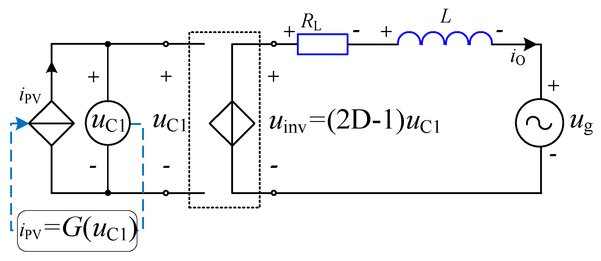
The output of the photovoltaic array has strongly nonlinear characteristics. The inverter circuit contains power switching devices, which is also a typical strongly nonlinear circuit. Therefore, the photovoltaic grid-connected inverter model, Equation (6), is a nonlinear model. The accuracy of the model is very important for the optimal design of the controller and the stability analysis of the system.

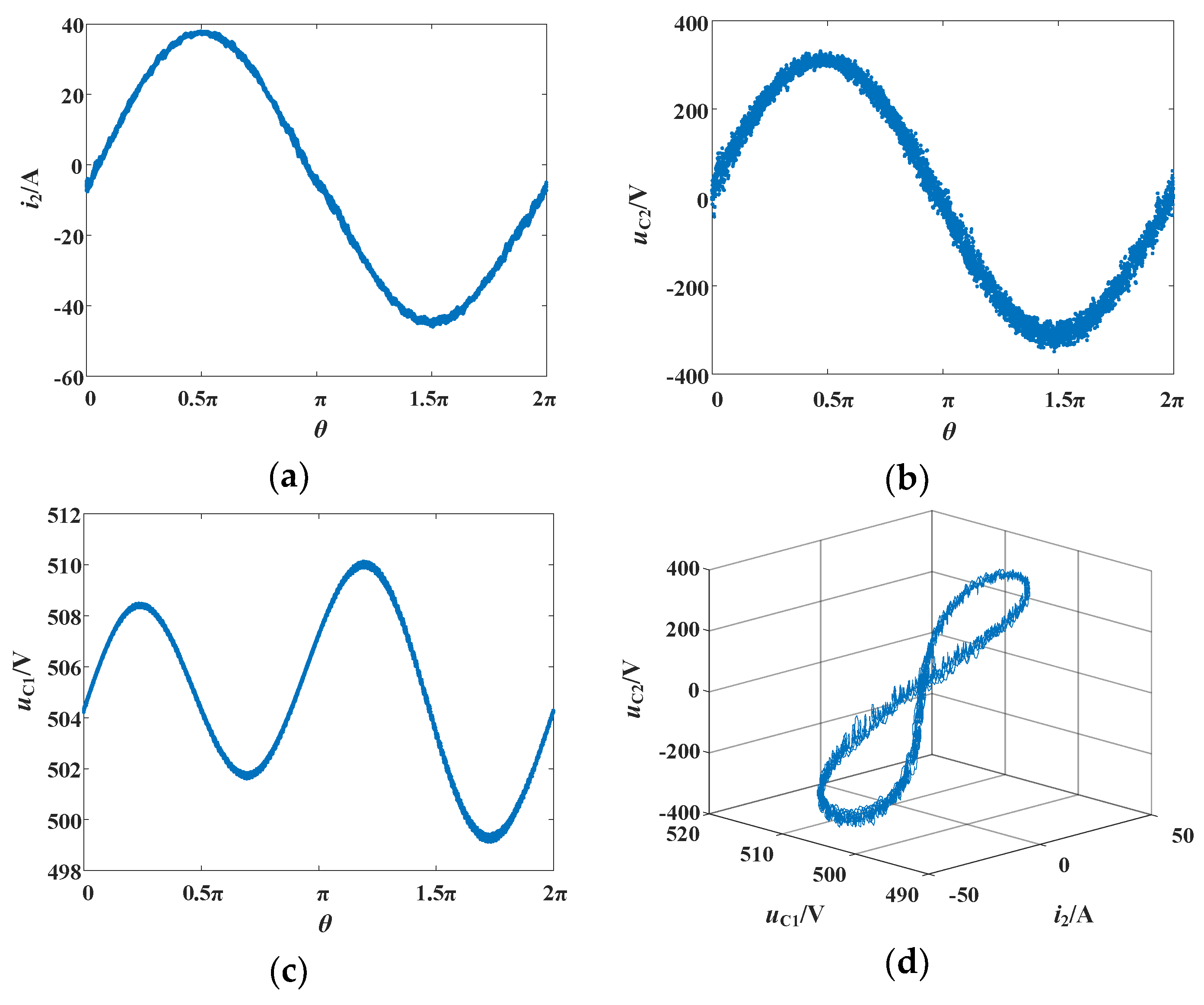
Figure 6 and Figure 7 provide analyses of the fast-scale bifurcations of photovoltaic grid-connected inverters with folded diagrams. They show that at certain parameter values, the system is in quasiperiodic and chaotic motion states. Fast-scale bifurcation analysis can be used to understand the dynamic behavior of each phase of the system state variable in the entire power frequency cycle with specific parameters for photovoltaic grid-connected inverters.

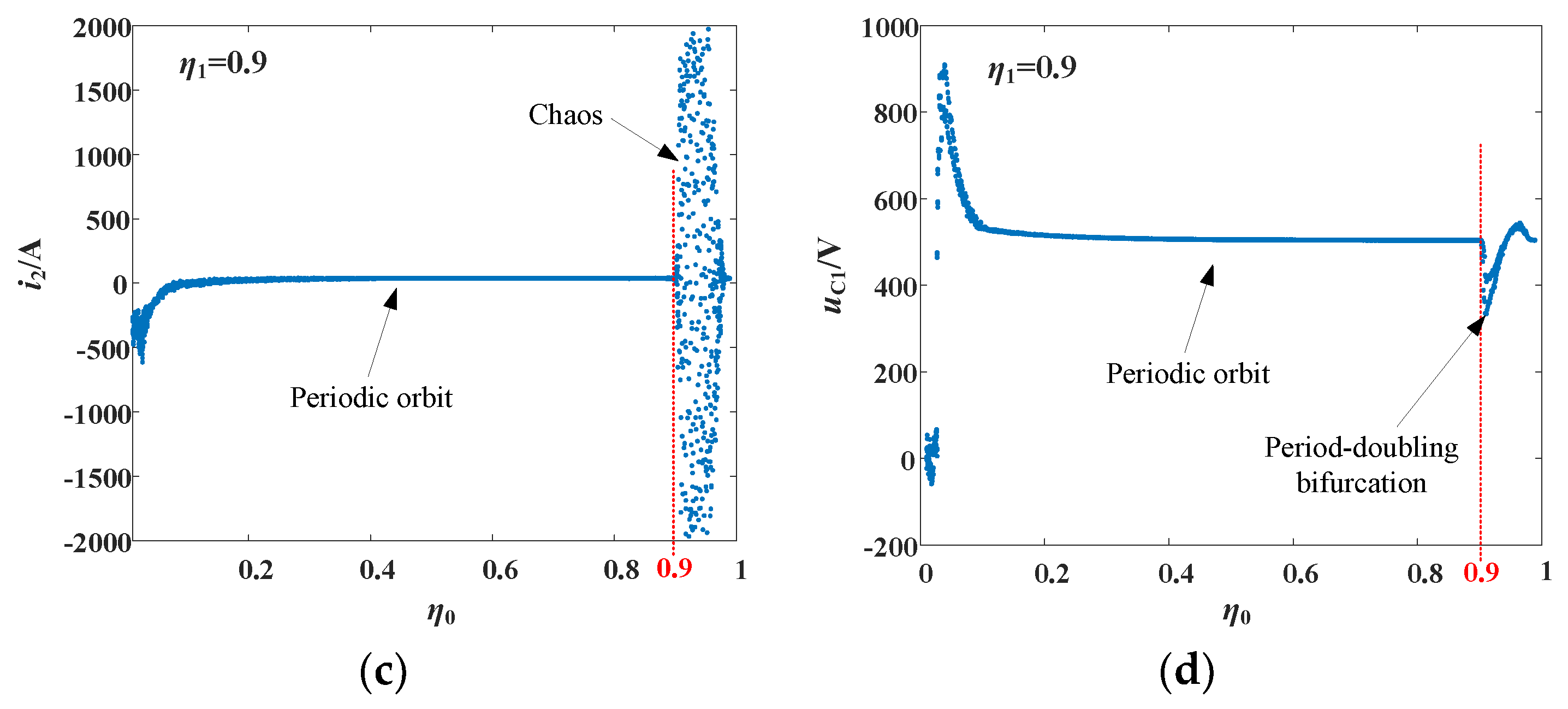
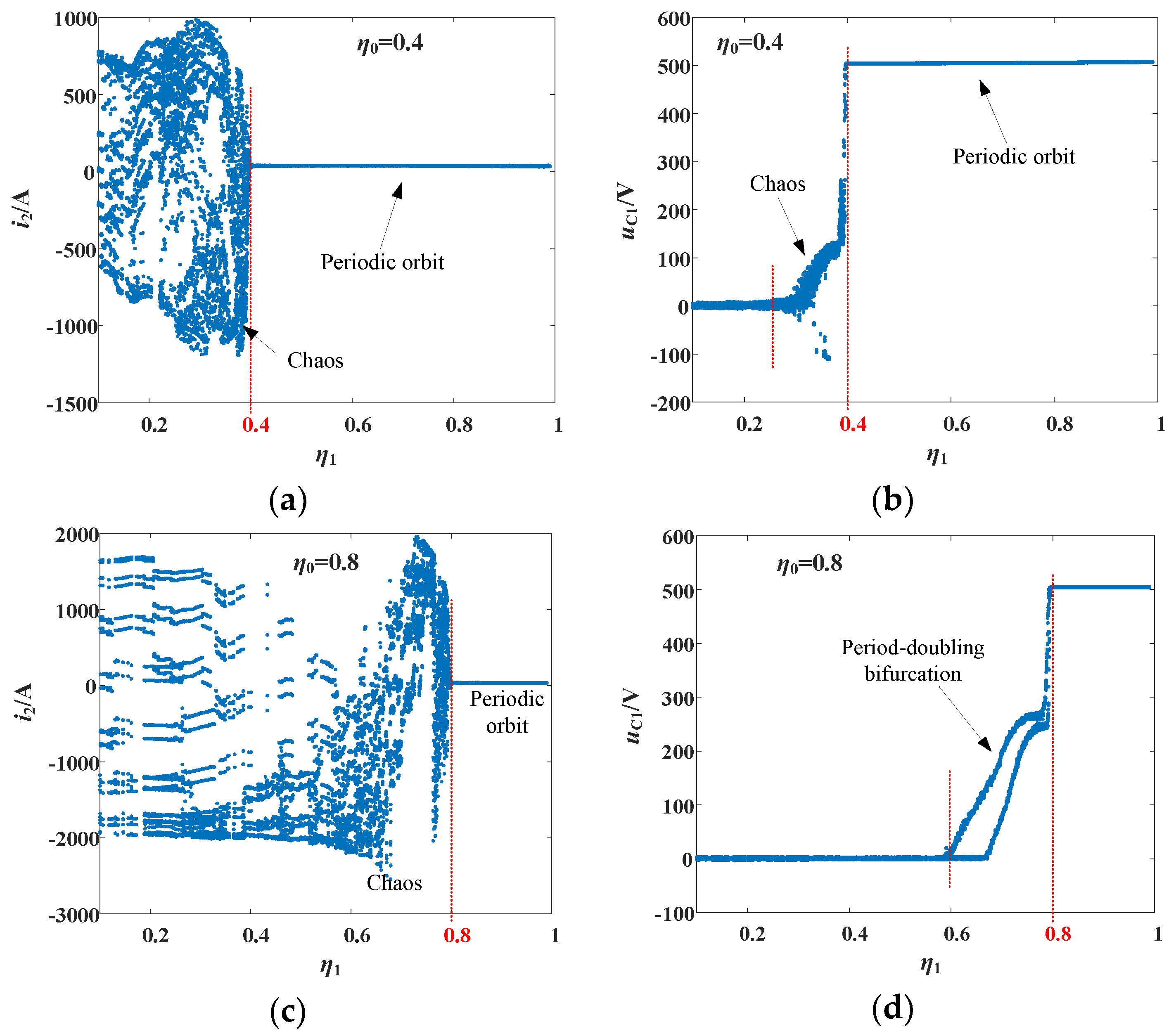
Figure 8 and Figure 9 show the bifurcation and chaos phenomena of the system using slow-scale bifurcation diagrams. It shows that as the control parameters change, the system switches between periodic, bifurcation, and chaotic motion states. The analysis of slow-scale bifurcation can be used to understand the influence of the changes in control parameters on the nonlinear dynamic behavior of the system, and it can also be used as a design guide for control parameters.

Figure 8 and Figure 9 indicate that when using ${\mathsf{\eta }}_0\left({\mathsf{\eta }}_1\right)$ as the bifurcation parameter, the value of ${\mathsf{\eta }}_1\left({\mathsf{\eta }}_0\right)$ affects the size of the chaotic motion window of the system. Therefore, in order to fully understand the influence of control parameters on the nonlinear dynamic behavior of the system, a three-dimensional bifurcation diagram, as shown in Figure 10, is constructed using ${\mathsf{\eta }}_0$ and ${\mathsf{\eta }}_1$ as the bifurcation parameters. The top view of the three-dimensional bifurcation diagram as shown in Figure 10b clearly shows the parameter area corresponding to the chaotic motion and periodic motion of the system. This servers as the guidance for selection of control parameters.

Figure 10. (a) Three-dimensional bifurcation diagram and (b) its top view with both ${\mathsf{\eta }}_0$ and ${\mathsf{\eta }}_1$ being bifurcation parameters.

When designing a controller, the control parameters ${\mathsf{\eta }}_0$ and ${\mathsf{\eta }}_1$ should be selected from the area of the periodic orbits shown in Figure 10b to ensure that the system is in a periodic motion state. In the design, the parameter values can be further optimized according to the objectives. Taking the reduction of the total harmonic distortion (THD) of the output current as an example, just take the parameter corresponding to the minimum value of THD from the output current THDs of the inverter calculated in the area of the periodic orbits shown in Figure 10b. A specific case is as follows. 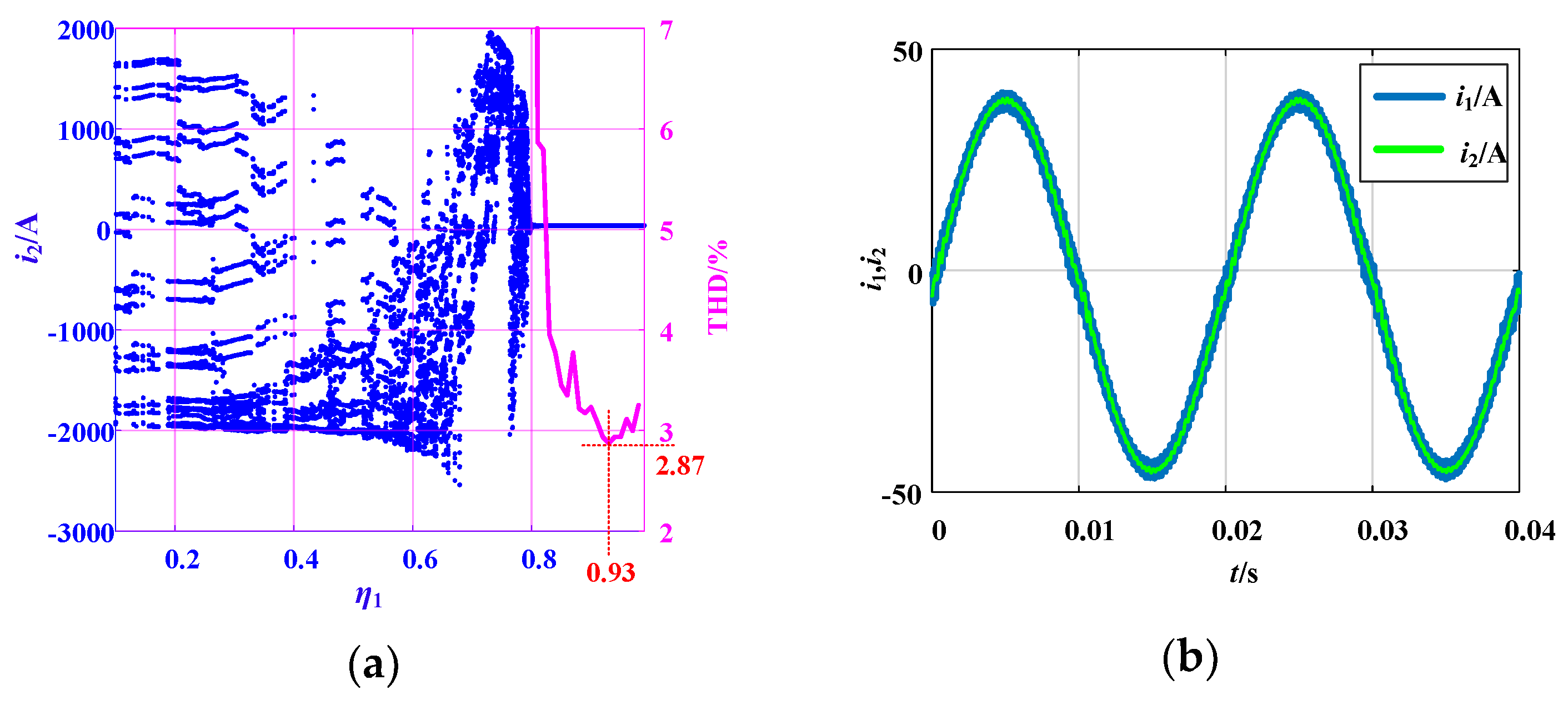Figure 11a shows the method of parameter selection through the bifurcation diagram and the total harmonic distortion. Let ${\mathsf{\eta }}_0$=0.8 and ${\mathsf{\eta }}_1$ be the bifurcation parameters; for example, when ${\mathsf{\eta }}_1$ is in the range of 0.8–1.0, the system is in the periodic motion state. In the region of this periodic motion, the total harmonic distortion of the output current $i_2$ of the photovoltaic grid-connected inverter is calculated for each parameter value. The purple curve in Figure 11a shows that when the control parameter ${\mathsf{\eta }}_1$ is 0.93, the total harmonic distortion of $i_2$, at 2.87%, is at its lowest. Accordingly, the control parameters are selected as ${\mathsf{\eta }}_0=0.8$ and ${\mathsf{\eta }}_1=0.93$, and the time-domain waveform of the output current $i_2$ from the photovoltaic grid-connected inverter is shown in Figure 11b. Based on the control parameters selected in this example, a 1kW experimental prototype is used to verify the effectiveness of the controller, as shown in Figure 12. The parameters of the experimental prototype are shown in Table 2. The experimental results show that the output current of the inverter can track the voltage signal of the power grid well without obvious distortion. Take out the current signal and put it into Matlab (R2019a)/Simulink to calculate its THD, which is 2.95%.

Figure 11. Selection of control parameter. (a) The optimal parameter is selected through the bifurcation diagram and the total harmonic distortion; (b) The time-domain waveform of the output current corresponding to the selected control parameters.

Figure 12. A 1kW prototype experiment. (a) Experimental prototype; (b) Grid-connected current and grid voltage waveform.

Table 2. Parameters of the 1kW experimental prototype.

Parameter	Value
$L_1$/mH	2.4
$L_2$/mH	0.6
$C_1$/$\mu$F	4.7 × 103
$C_2$/$\mu$F	4.7
$f_{\mathrm{grid}}$/Hz	50
$f_{\mathrm{S}}$/ kHz	25
${\mathsf{\eta }}_0$	0.8
${\mathsf{\eta }}_1$	0.93
$I_{SC}^{ar}$/A	33.42
$U_{OC}^{ar}$/V	540.0

PV grid-connected inverter contains switching devices, which is a typical strong non-linear system. The existing research shows that the PV grid-connected inverter will appear bifurcation and chaos in a certain range of parameters. The non-linear dynamics of PV grid-connected inverter can be studied on two-time scales (switching frequency and grid line frequency) by fast and slow-scale bifurcations. When the system begins to bifurcate from periodic motion and then enters into chaos, it means that the system has begun to deteriorate and become unstable. These dynamic behaviors are related to system parameters, which include electronic component parameters and control parameters. The study of the relationship between the device and control parameters and the non-linear dynamic behavior can reveal the dynamic behavior of the PV grid-connected inverter, guide the developers to choose the correct parameter range, and guide the controller design. The study of non-linear dynamic behavior can lead a perspective to study the design and stability of PV grid-connected inverter, which is complementary to the classical linear control theory, and provides analysis methods and tools for the design of PV grid-connected inverter.

6. Conclusions

A photovoltaic grid-connected inverter is a strongly nonlinear system, so it is of great significance to establish its nonlinear model for analysis. To improve the modeling accuracy, in this study we have comprehensively considered the nonlinear characteristics of photovoltaic arrays and the strongly nonlinear characteristics of switching circuits, established a nonlinear model of photovoltaic grid-connected inverters, and solved its predictive controller. We have analyzed the model by using folded diagrams, phase diagrams, and bifurcation diagrams. We have studied the nonlinear dynamic behavior of photovoltaic grid-connected inverters under predictive control on both fast and slow scales. Our studies have shown that bifurcation and chaotic behaviors exist in photovoltaic grid-connected inverters under a certain range of control parameters. By analyzing the inherent relationship between the control parameters and the nonlinear dynamic behavior characteristics, we can select and optimize the control parameters in the design of grid-connected inverters. Based on this work, future studies can further explore random fluctuations of the power grids, local loads, photovoltaic arrays under the influence of the environment, and the network structure characteristics of the new smart grid, thus yielding additional insights into the stability and interaction mechanisms of photovoltaic grid-connected inverters and power grids.

References

1. Sarmiento, J.E.; Carreno, E.M.; Zambroni de Souza, A.C. Modeling inverters with volt-var functions in grid-connected mode and droop control method in islanded mode. Electr. Power Syst. Res. 2018, 155, 265–273. [Google Scholar] [CrossRef]
2. Trujillo, C.L.; Santamaría, F.; Gaona, E.E. Modeling and testing of two-stage grid-connected photovoltaic micro-inverters. Renew. Energy 2016, 99, 533–542. [Google Scholar] [CrossRef]
3. Wang, Y.; Chen, X.; Wang, Y.; Gong, C. Analysis of frequency characteristics of phase-locked loops and effects on stability of three-phase grid-connected inverter. Int. J. Electr. Power Energy Syst. 2019, 113, 652–663. [Google Scholar] [CrossRef]
4. Errouissi, R.; Muyeen, S.M.; Al-Durra, A.; Leng, S. Experimental Validation of a Robust Continuous Nonlinear Model Predictive Control Based Grid-Interlinked Photovoltaic Inverter. IEEE Trans. Ind. Electron. 2016, 63, 4495–4505. [Google Scholar] [CrossRef] [Green Version]
5. Liao, Z.X.; Luo, X.S. Research on synchronous method for photovoltaic supplied micro-grid based on small-world network model. Acta Phys. Sin. 2014, 63, 230502. [Google Scholar] [CrossRef]
6. Akhavan, A.; Mohammadi, H.R.; Guerrero, J.M. Modeling and design of a multivariable control system for multi-paralleled grid-connected inverters with LCL filter. Int. J. Electr. Power Energy Syst. 2018, 94, 354–362. [Google Scholar] [CrossRef] [Green Version]
7. Babu, B.C.; Gurjar, S. A Novel Simplified Two-Diode Model of Photovoltaic (PV) Module. IEEE J. Photovolt. 2014, 4, 1156–1161. [Google Scholar] [CrossRef]
8. Mahmoud, Y.; El-Saadany, E.F. A Photovoltaic Model with Reduced Computational Time. IEEE Trans. Ind. Electron. 2015, 62, 3534–3544. [Google Scholar] [CrossRef]
9. Mahmoud, Y.; Xiao, W. Evaluation of Shunt Model for Simulating Photovoltaic Modules. IEEE J. Photovolt. 2018, 8, 1818–1823. [Google Scholar] [CrossRef]
10. Liao, Z.X.; Luo, X.S.; Huang, G.X. Numerical modeling and research on nonlinear dynamic behaviors of two-stage photovoltaic grid-connected inverter. Acta Phys. Sin. 2015, 64, 130503. [Google Scholar] [CrossRef]
11. Liu, H.C.; Yang, S. Study on bifurcation and chaos in single-phase H-bridge inverter modulated by unipolar sinusoidal pulse width modulation. Acta Phys. Sin. 2013, 62, 210502. [Google Scholar] [CrossRef]
12. Tong, Y.N.; Li, C.L.; Zhou, F. Synchronization control of single-phase full bridge photovoltaic grid-connected inverter. Optik 2016, 127, 1724–1728. [Google Scholar] [CrossRef]
13. Xie, R.L.; Hao, X.; Wang, Y.; Yang, X.; Huang, L.; Wang, C.; Yang, Y.H. An exact discrete-time model and the bifurcation performance of single phase grid-connected inverter with L-filter considering dead-time nonlinearity. Acta Phys. Sin. 2014, 63, 120510. [Google Scholar] [CrossRef]
14. Hamill, D.C.; Deane, J.H.B.; Jefferies, D.J. Modeling of chaotic DC-DC converters by iterated nonlinear mappings. IEEE Trans. Power Electron. 1992, 7, 25–36. [Google Scholar] [CrossRef]
15. Fan, J.W.; Chung, H.S. Bifurcation Phenomena and Stabilization with Compensation Ramp in Converter with Power Semiconductor Filter. IEEE Trans. Power Electron. 2017, 32, 9424–9434. [Google Scholar] [CrossRef]
16. Luo, X.S.; Wang, B.H.; Chen, G.R.; Quan, H.J.; Fang, J.Q.; Zou, Y.L.; Jiang, P.Q. Research on bifurcation behaviour and chaos control in DC-DC buck converter. Acta Phys. Sin. 2003, 52, 12. [Google Scholar] [CrossRef]
17. Lenz Cesar, E.; Pagano, D.J.; Pou, J. Bifurcation Analysis of Parallel-Connected Voltage-Source Inverters with Constant Power Loads. IEEE Trans. Smart Grid 2018, 9, 5482–5493. [Google Scholar] [CrossRef]
18. Wei, D.Q.; Wan, L.; Luo, X.S.; Zeng, S.Y.; Zhang, B. Global exponential stabilization for chaotic brushless DC motors with a single input. Nonlinear Dyn. 2014, 77, 209–212. [Google Scholar] [CrossRef]
19. Wei, D.Q.; Zhang, B. Controlling chaos in permanent magnet synchronous motor based on finite-time stability theory. Chin. Phys. B 2009, 18, 1399–1403. [Google Scholar]
20. Aditya, K.; Williamson, S.S. Design Guidelines to Avoid Bifurcation in a Series–Series Compensated Inductive Power Transfer System. IEEE Trans. Ind. Electron. 2019, 66, 3973–3982. [Google Scholar] [CrossRef]
21. Shuai, Z.K.; Hu, Y.; Peng, Y.L.; Tu, C.M.; Shen, Z.J. Dynamic Stability Analysis of Synchronverter-Dominated Microgrid Based on Bifurcation Theory. IEEE Trans. Ind. Electron. 2017, 64, 7467–7477. [Google Scholar] [CrossRef]
22. Huang, J.H.; Yang, J.H.; Xie, D.S.; Wu, D.Q. Optimal Sliding Mode Chaos Control of Direct-Drive Wave Power Converter. IEEE Access 2019, 7, 90922–90930. [Google Scholar] [CrossRef]
23. Morcillo, J.D.; Burbano, D.; Angulo, F. Adaptive Ramp Technique for Controlling Chaos and Subharmonic Oscillations in DC–DC Power Converters. IEEE Trans. Power Electron. 2016, 31, 5330–5343. [Google Scholar] [CrossRef]