Article

Failure Prediction of the Rotating Machinery Based on CEEMDAN-ApEn Feature and AR-UKF Model

1
School of Electrical Engineering and Automation, Harbin Institute of Technology, Harbin 150080, China
2
China Institute of Marine Technology and Economy, Beijing 10001, China
*
Author to whom correspondence should be addressed.
Appl. Sci. 2020, 10(6), 2056; https://doi.org/10.3390/app10062056
Submission received: 17 February 2020 / Revised: 16 March 2020 / Accepted: 17 March 2020 / Published: 18 March 2020
(This article belongs to the Special Issue Machine Fault Diagnostics and Prognostics)

Abstract

:
A novel failure prediction method of the rotating machinery is presented in this paper. Firstly, the complete ensemble empirical mode decomposition with adaptive noise (CEEMDAN) is applied to decompose the vibration signals of the rotating machinery into a number of intrinsic mode functions (IMFs) and a residual (Res), and the metric of maximal information coefficient (MIC) is used to select eligible IMFs to reconstruct signals. Then, the approximate entropy (ApEn)-weighted energy value of the reconstructed signals are calculated to track the degradation process of the rotating machinery. Furthermore, the Chebyshev inequality is introduced to determine the prediction starting time (PST). Finally, the auto regress (AR) model and unscented Kalman filter (UKF) algorithm are used to predict the remaining useful life (RUL) of the rotating machinery. The method is fully evaluated in a test-to-failure experiment. The obtained results show that the proposed method outperforms its counterparts on failure prediction of the rotating machinery.

1. Introduction

With the development of material science and ultra-micro fabrication techniques, the rotating machinery plays an more and more vital role in modern industry. However, the performance of the rotating machinery would always deteriorate with time, which results in the potential for failure occurrence. Once the failure occurs, it will not only cause huge economic losses but also lead to catastrophic casualties and severe social impacts [1,2]. Consequently, it is important and significant to address the failure prediction issue of the rotating machinery.
Generally speaking, the failure prediction process of the rotating machinery is commonly divided into the two stages: the fault feature extraction stage and the remaining useful life (RUL) prediction stage. Theoretically, the main methods for extracting fault features of the rotating machinery can be classified into three types: time domain, frequency domain, and time-frequency domain. Root mean square (RMS), skewness, and kurtosis are common features of time domain methods [3]. Kurtosis is commonly used to identify early fault because of its high sensitivity [4]. RMS is insensitive to early fault, but it shows strong stability on describing the degradation process of the rotating machinery [5]. Heng et al. first tracked the degradation of the rotating machinery with kurtosis and skewness [6]. Features of time domain possess many merits, such as simple in computation and clear in conception, but they are susceptible to noises. Frequency domain methods are mainly based on Fast Fourier Transform (FFT); thus, center frequency and RMS of frequency are frequently used features. FFT is an averaged chirp frequency feature representation of the signals over the entire time period. Therefore, it cannot reflect frequency domain features of the signals in the local time region, so it is confined for the analysis of the stationary signals. Recently, the time-frequency domain analysis method is a hot spot in this field. Empirical mode decomposition (EMD) [7,8,9,10], wavelet (WT) [11,12,13,14,15], and neural network (NN) [16,17,18] are common means to extract time-frequency features. Qian et al. used the improved recursive entropy as a health indicator for the performance degradation of bearings [19]. Rai and Upadhyay combined the ensemble empirical mode decomposition (EEMD) with the energy moment entropy to track the degradation process of bearings [20,21,22]. However, the above three types of methods are based on the assumption of linearity. To some extent, vibration signals of the rotating machinery always show a certain degree of non-stationarity and non-linearity because of the constantly changing frictional forces, resistance forces, and loads between components of the rotating machinery.
Currently, RUL prediction methods can be categorized into two kinds: model-based and data-driven. The former has to set up a mathematical or physical model which can express the degradation process of the rotating machinery. Liao et al. [23] and Oppenheimer et al. [24] adopted the Paris crack growth model and the Forman crack growth model to predict RUL with the measured data, respectively. Model-based methods can accurately describe the developing trend of damage variables of the rotating machinery according to certain physical laws. However, most mathematical or physical models can’t be updated over time, which will result the poor universality. Recently, data-driven methods have become the research focus because they only need the historical data. Therefore, they are quite applicable to the prediction of complex systems for its adjustability. Kalman filter [25,26], Bayesian network [21], and support vector machine [27] (SVM) are typical data-driven methods used for the RUL prediction of the rotating machinery. However, all above methods are still suffering from the deficiencies of low accuracy and the requirements of numerous historical data for training.
Aiming at shortcomings of existing failure prediction methods, this paper proposes an effective method to track the degradation process and predict the remaining useful life of the rotating machinery. The main innovation of this paper is summarized as follows.
(1)
The complete ensemble empirical mode decom-posetion with adaptive noise (CEEMDAN), which can overcome shortages of EMD and EEMD on modal aliasing and calculation efficiency, is adopted to decompose the original vibration signals of the rotating machinery into a number of IMFs and a residual.
(2)
The maximal information coefficient (MIC), which can reveal the degree of association between two variables, is utilized to select eligible IMFs and get the reconstructed signals.
(3)
The approximate entropy (ApEn) is employed to achieve fault features of the reconstructed signals and track the degradation process of the rotating machinery.
(4)
A remaining useful life (RUL) prediction model by combing the auto regress (AR) model and the unscented Kalman filter (UKF) algorithm is developed to achieve the RUL of the rotating machinery accurately.
The paper is organized as follows. Following with the introduction, Section 2 describes details of the proposed failure prediction method. Section 3 gives the experimental results to show the effectiveness of the proposed method. The final section summarizes the conclusions drawn from the results.

2. Methodology

2.1. Overview

The proposed method aims at addressing the failure prediction problem of the rotating machinery accurately, and its functional block diagram, is shown in Figure 1.
Considering that the original signals measured by the vibration sensors have much noise interference, CEEMDAN and MIC are thus used to obtain the reconstructed signals in the fault feature extraction stage. Then, ApEn of the reconstructed signals is achieved as the health indicator of the rotating machinery. Details of the fault feature extraction are described in Section 2.2.
The prediction starting time, on which the rotating machinery has a slight failure but can work for a longer period, is achieved with the Chebyshev inequality. By selecting a reasonable final failure threshold according to the actual situation, all time slots for performing RUL prediction can be identified. More details about initial and final failure prediction are described in Section 2.3.
In the remaining life prediction stage, an efficient RUL prediction model by the combination of the AR model and UKF algorithm is developed to accurately obtain the RUL of the rotating machinery. More details about the RUL prediction are described in Section 2.4.

2.2. Fault Feature Extraction Stage

Due to the changing frictional forces, resistance forces, and loads between components of the rotating machinery, the vibration signals present nonlinear and noise disturbance characteristics. Therefore, it is necessary to diminish the disturbing of the noise under nonlinear condition and fetch the helpful information. In fault feature extraction stage, CEEMDAN is applied to decompose the vibration signals of the rotating machinery into a number of IMFs and a residual.
In general, only parts of the IMFs are sensitive to the failure. To diminish the disturbing of the noise effectively, MIC is used to select eligible IMFs to reconstruct signals with helpful information.
To describe the degradation process accurately, ApEn-weighted energy value of the reconstructed signals is used to track the degradation process of the rotating machinery. In other words, CEEMDAN-ApEn is the feature proposed for RUL prediction in this paper.

2.2.1. Complete Ensemble Empirical Mode Decomposition with Adaptive Noise

Compared with the white Gaussian noise adopted in EMD and EEMD, CEEMDAN adds the specific noise to each step of its decomposition to overcome shortcomings of EMD [28,29] and EEMD [30]. Concretely, the IMF is achieved as the difference between the current residual and its local mean. The number of CEEMDAN iterations is half that of EEMD, and it can accurately decompose the signals. The process of CEEMDAN is described as follows:
(1)
Add F k ω i to the original signals X:
X i = X + β k 1 F k ω i ,
where F k ω i is the k-th IMF processing Gaussian white noise, and β k 1 is the signal-to-noise radio for each procedure.
(2)
Use EMD to obtain the local mean of X i to get the first residual r 1 :
r 1 = 1 N i = 1 N H x i ,
where N is total number of sets, and H is a function used to estimate the local mean of signals.
(3)
Calculate the first IMF:
I M F 1 = X r 1 .
(4)
Decompose r 1 + β 1 F 2 ω i and delimit the second IMF:
I M F 2 = r 1 r 2 = r 1 1 N i = 1 N H r 1 + β 1 F 2 ω i .
(5)
Calculate the k-th residual r k :
r k = 1 N i = 1 N H r k 1 + β k 1 F k ω i .
(6)
Get k-th IMF:
I M F k = r k 1 r k .
(7)
Repeat Equations (5) and (6) steps until R meets the terminal condition:
R = X k = 1 K I M F k .
Therefore, X can be expressed as Equation (8), and all IMFs can be described as Y = I M F k , k = 1 , 2 , , K .
X = R + k = 1 K I M F k .

2.2.2. Maximal Information Coefficient

As a relationship measurement method, the maximal information coefficient (MIC) is proposed by Reshef et al. [31] to reveal the correlation of variables. Therefore, MIC is applied to perform selection of IMFs which achieved by CEEMDAN. The details of MIC are described as follows.
(1)
Denote p y 1 , y 2 as a joint probability distribution function of two variables y 1 and y 2 , and mutual information of y 1 and y 2 is defined as:
I y 1 , y 2 = y 1 y 2 p y 1 , y 2 log p y 1 , y 2 p y 1 p y 2 d y 1 d y 2 ,
where p y 1 and p y 2 denote the marginal probability distribution function of y 1 and y 2 , respectively. I y 1 , y 2 is non-negative and I y 1 , y 2 = 0 iff p y 1 , y 2 = p y 1 p y 2 . It is obviously that the value of I is higher than zero when y 1 and y 2 are correlated, and the stronger the correlation is, the larger the value of I y 1 , y 2 .
(2)
Suppose Y is consisted of a number of elements which are ordered value pairs of y 1 and y 2 , and N is the amount of pairs. A grid G is defined as a partition on Y, which can partition the values of y 1 in Y into a number of n y 1 bins and that of y 2 in Y into a number of n y 2 bins, respectively. Denote I y 1 , y 2 , Y | n y 1 , n y 2 as the mutual information of y 1 and y 2 on grid G with n y 1 rows and n y 2 columns. The feature matrix of Y is defined as:
Υ y 1 , y 2 | Y n y 1 , n y 2 = I * y 1 , y 2 , Y , n y 1 , n y 2 log min n y 1 , n y 2 ,
where I * y 1 , y 2 , Y , n y 1 , n y 2 = I y 1 , y 2 , Y | G , n y 1 , n y 2 represents the maximum mutual information of y 1 and y 2 on grid G.
(3)
Furthermore, MIC of y 1 and y 2 in set Y with N samples is defines as follows.
M y 1 , y 2 | Y = max n y 1 × n y 2 < θ N Υ y 1 , y 2 | Y n y 1 , n y 2 ,
where θ N is the upper bound of the grid size required to be selected carefully, and its suitable value is θ N = N 0.6 .
By calculating the MIC value between each IMF and the original signals according to above steps, IMF with MIC value larger than a threshold is selected as the eligible one, and it is added into a set of IMF Z. Then, the signals U with helpful information can be reconstructed with all eligible IMFs in Z.

2.2.3. Approximate Entropy

Pincuss et al. proposed the concept of the approximate entropy (ApEn) to quantitatively describe the complexity of the signals [32]. The approximate entropy is less dependent on the amount of data, and its value is stable, and non-stationary. Today, ApEn is widely used in engineering applications. The larger the value of ApEn, the more complicated the given time series is.
Denote U = u i , i = 1 , 2 , , N as the signals; m and r are the pattern dimension and the similarity tolerance, which are given in advance. The value of ApEn can be obtained by the following steps.
(1)
The sequence u i is sequentially composed into an m-dimensional vector P i :
P i = u i , u i + 1 , , u i + m 1 s . t . i = 1 , 2 , , N m + 1 .
(2)
Calculate the distance between the vector P i and the remaining vectors P j for each i.
d P i , P j = max k u i + k u j + k .
(3)
Given a threshold r r > 0 , for each value of i, count the number n of d P i , P j < r and calculate the ratio c i m r of n to the total number N m + 1 .
c i m r = n N m + 1 .
(4)
Calculate the logarithm of c i m r and get it average value ϕ m r :
ϕ m r = 1 N m + 1 i = 1 N m + 1 ln c i m r .
(5)
Add the dimension to m + 1 , and repeat steps (1)–(4) to get ϕ m + 1 r .
(6)
The value of ApEn for this sequence is:
E m , r , N = lim N ϕ m + 1 r ϕ m r .
In actual calculation, N is a finite value; thus, the estimation value of ApEn estimate can be expressed as:
E m , r , N = ϕ m + 1 r ϕ m r .
Generally speaking, the values of parameters are set to m = 2 and r = 0.1 0.2 S D u , where S D represents the standard deviation. By calculating the value of ApEn of the reconstructed signals U, the proposed feature named CEEMDAN-ApEn is achieved, and it is used as the health indicator of the rotating machinery.

2.3. Initial and Final Failure Prediction Stage

Throughout the life cycle, the rotating machinery will degrade continuously over time, and gradually deteriorate from the healthy state to the failure state over a long period. Therefore, an appropriate threshold should to be selected to identify the beginning of the degradation process. In this paper, Chebyshev inequality is adopted to select the threshold of the initial failure.
p E μ k σ k 2 σ k 2 ε k 2 ε k 2 ,
where E is the CEEMDAN-ApEn feature sequence of the rotating machinery in the same state, μ k and σ k are the mean and the standard deviation of E, respectively, and ε k is a real number.
In theory, Chebyshev inequality shows that for an observation sequence of the same state with a probability distribution, all values in the sequence are close to the mean of the sequence. Therefore, the probability that all sequence values drops into interval μ k ε k , μ k + ε k is greater than 1 σ k 2 σ k 2 ε k 2 ε k 2 . This theory can be illustrated by the following hypothesis testing methods:
H 0 : E μ k < ε k H 1 : E μ k > ε k .
Denote E 0 as a value of the CEEMDAN-ApEn feature in healthy state. When E 0 μ k ε k , the first type of mistake will be made if we reject the hypothesis H 0 and identify the rotating machinery as the failure state. According to the Chebyshev inequality, the probability of making above mistake is α = σ k 2 σ k 2 ε k 2 ε k 2 . By contrast, suppose E 1 is a value of the CEEMDAN-ApEn feature in failure state. When E 1 μ k < ε k , the second type of mistake will be made if we accept the hypothesis H 0 and identify the rotating machinery as the healthy state, and the probability of making above mistake is β . If α is too large, the healthy state of the rotating machinery would be mistaken as the failure state. On the contrary, if β is too large, the failure state of the rotating machinery would be mistaken as the healthy state.
In practical applications, priority should be given to the prevention of the first type of mistake. Therefore, we set ε k = 5 σ k by α = 4 % , which means that the value of CEEMDAN-ApEn feature of the rotating machinery in the healthy state would fall into the interval μ k 5 ε k , μ k + 5 ε k with a confidence probability of 96%. In other words, once the value of the CEEMDAN-ApEn feature exceeds the threshold μ k + 5 ε k , it should be considered that the rotating machinery is already in failure state. Therefore, μ k + 5 ε k is the identification for the beginning of the degradation process, and prediction starting time is the time on which the value of RUL exceeds μ k + 5 ε k for the first time.
Final failure means the end of the rotating machinery. Therefore, it is necessary to determine a threshold to identify the time of the final failure. Based on the analysis of the references in this field [33,34], the threshold of the final failure ζ is usually selected according to the practice and experience. In details, the value of the health indicator shows a sudden change when a fault occurs, which can be used as the basis for the selection of ζ .

2.4. RUL Prediction

2.4.1. Unscented Kalman Filter

The Unscented Kalman Filter (UKF) is an algorithm which can approximate the probability density function of variables. Based on the unscented transformation and Kalman linear filtering framework, UKF can address the particle degradation problem with deterministic sampling strategy. Details of UKF is introduced as follows.
A matrix Q with 2 n + 1 elements (sigma points) is generated as follows.
Q i = μ q , i = 0 μ q + n + λ c q , i = 1 , 2 , , n μ q n + λ c q , i = n + 1 , n + 2 , , 2 n ,
where μ q and c q are the mean and the covariance of n-dimensional random variables. λ = α 2 n + κ n is the scale factor, where κ should satisfy the condition of the matrix n + λ c q being a semi positive definite matrix.
Then, each sigma point should be modified as follows.
W j = λ λ n + λ , j = 0 n + λ , j = 0 1 1 2 n + λ , j = 1 , 2 , , 2 n 2 n + λ , j = 1 , 2 , , 2 n W c j = λ λ n + λ + 1 σ 2 + β , j = 0 n + λ + 1 υ 2 + τ , j = 0 1 1 2 n + λ , j = 1 , 2 , , 2 n 2 n + λ , j = 1 , 2 , , 2 n
where W j and W c j represent the weights of mean and covariance, respectively. υ is the zooming factor, and τ contains higher order moment information for the prior distribution.
Suppose the state space model of the nonlinear system is as follows.
s k + 1 = f s k + w k ,
o k = h s k + v k ,
where s k is n-dimensional state vector, and o k is observation vector. f and h are the state transition function and measurement function, respectively. w k and v k represent uncorrelated zero-mean white noise, in which the covariance is c s k and c o k , respectively.
Suppose O i = f S i is the output of above nonlinear system with the input S i , and μ o and c o are its mean and covariance, respectively. UKF is divided into a prediction step and an update step. The prediction step is introduced as follows:
S k | k 1 i = f S k 1 | k 1 i , i = 0 , 1 , , 2 n ,
O k | k 1 i = h S k | k 1 i , i = 0 , 1 , , 2 n ,
s ^ k | k 1 = i = 0 2 n W i S k | k 1 i ,
o ^ k | k 1 = i = 0 2 n W i O k | k 1 i ,
c k | k 1 = c s k + i = 0 2 n W c i S k | k 1 i s ^ k | k 1 S k | k 1 i s ^ k | k 1 T .
The update step is described as follows.
c o = c o k + i = 0 2 n W c i O k | k 1 i o ^ k | k 1 O k | k 1 i o ^ k | k 1 T ,
c s o = i = 0 2 n W c i S k | k 1 i s ^ k | k 1 O k | k 1 i o ^ k | k 1 T ,
K k = c s o c o 1 ,
s ^ k | k = s ^ k | k 1 + K k o k o ^ k | k 1 ,
c k | k = c k | k 1 K k c o K k T .

2.4.2. AR-UKF Prediction Model

To predict RUL of the rotating machinery, the state transition function, which can accurately describe the entire degradation process, should be set up in advance. In fact, the state of the rotating machinery behaves in temporal correlation; thus, the value of the health indicator of the current time depends on that of the previous time. Therefore, the Autoregressive (AR) model, which can predict of the future data of the random variable using its historical data, is adopted to set up the state transition function as follows.
s k = j = 1 p a j s k j + w k 1 ,
where a j j = 1 , 2 , , p is the coefficient which indicates the importance of each historical data on generating the prediction data. p is the order of the AR model, which can be achieved by applying AIC rule and Burg algorithm. w is the process noise.
Furthermore, the measurement function is introduced as follows.
o k = s k + v k
where v is the measurement noise. To predict RUL of the rotating machinery, it is necessary to calculate the actual state s by using the observation o.
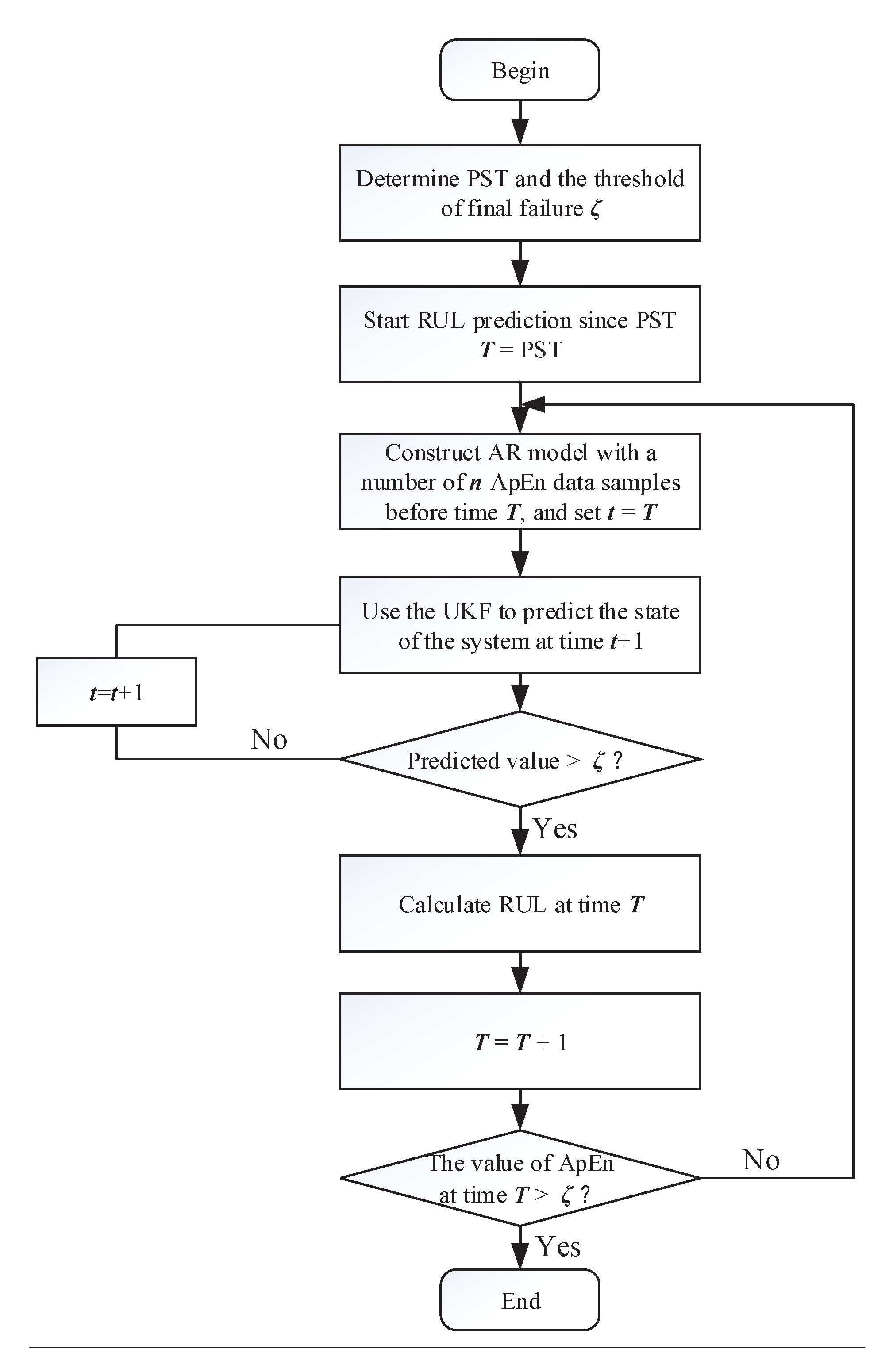
In this paper, UKF is adopted to estimate the state of the rotating machinery with the proposed CEEMDAN-ApEn feature. The flow diagram of the proposed AR-UKF prediction model is shown in Figure 2, and its specific steps are as follows.
(1)
Calculate the proposed CEEMDAN-ApEn feature according to the method proposed in Section 2.2. Obtain the prediction starting time (PST) and the threshold of the final failure using the method proposed in Section 2.3.
(2)
Start RUL prediction by setting T = PST .
(3)
At the time T, select n data samples of the CEEMDAN-ApEn feature on time slots T n + 1 , T n + 2 , , T to construct the AR model.
(4)
Use UKF to perform multiple steps prediction on time slots T + 1 , T + 2 , until the predicted value is greater than the threshold of final failure ζ . Suppose the time corresponding to above predicted value is T + m ; thus, m is the predicted RUL at the time T.
(5)
Repeat Equations (3) and (4) by setting T = T + 1 .
(6)
Finally, the predicted RUL value obtained at each time is used to plot a RUL curve.

3. Experiment and Results

3.1. Experimental Setup

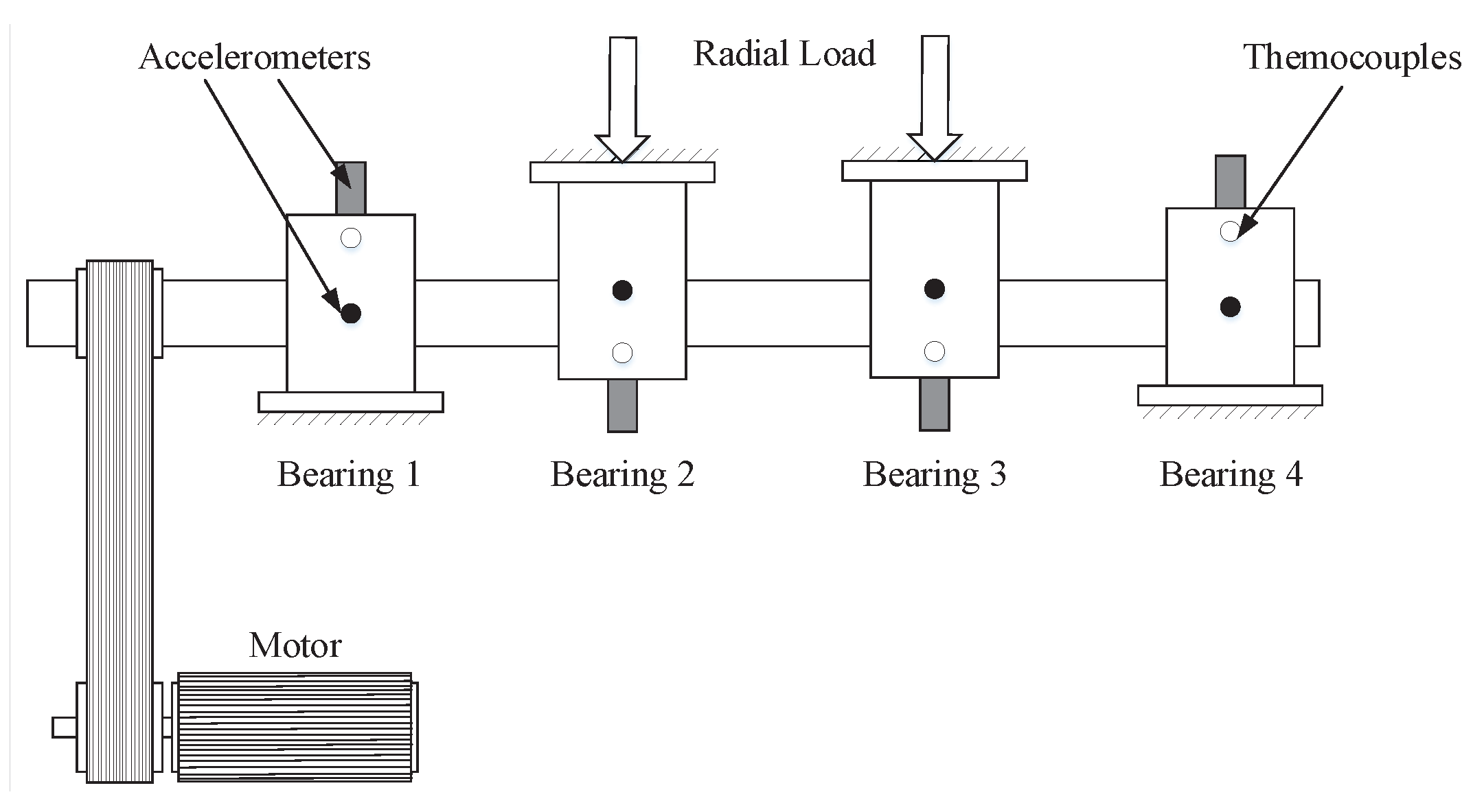
To verify the ability of the proposed method on failure prediction of the rotating machinery, vibration signals data collected by the NSF I/UCR Center are utilized in this paper. The framework of the experimental system is shown Figure 3. By using the spring mechanism, the system was run fixed at 2000 r/min, and a 6000-lb radial load was placed onto the shaft and bearing. Four bearings (bearings 1–4, model: ZA-2115, 16 rollers in each row, pitch diameter: 2.815 in, roller diameter: 0.331 in, tapered contact angle: 15.17 ° ) were installed on the shaft, and lubricated with an oil circulation system that regulated the flow and the temperature of the lubricant. A magnetic plug installed in the oil feedback pipe was adopted to collect debris from the oil as evidence of the bearing degradation. When the accumulated debris adhered to the magnetic plug exceeded a certain level, the test terminated by turning off the power. Accelerometers (model: PCB 353B33 high sensitivity quartz ICP) were mounted on bearing housing and four thermocouples were attached to the outer race of each bearing to record the temperature. The vibration signals were collected by a data acquisition system. The sampling rate was fixed to 20 KHz, and 20,480 data points were recorded in each data file.
From 10:32, 12 February 2004 to 6:22, 19 February 2004, vibration signals of bearings were recorded in a number of 984 files with a time interval of 10 min. At the end of experiments, an outer race fault occurs in bearing 1.

3.2. Fault Feature Extraction and Selection

As mentioned in Section 2.2, CEEMDAN is applied to decompose the vibration signals X into a series of IMFs and a residual. It is well known that an eligible IMF contains helpful information of the original signals, which means they are strongly related. By contrast, an ineligible IMF has randomness and fuzziness, which means it is weakly related with the original signals. Considering that MIC can measure the strengthen of the correlation, it is thus adopted to determine the effectiveness of IMFs. Moreover, an appropriate threshold γ is introduced to select all eligible IMFs as follows.
γ = β × M X , Ω ,
where Ω is Gaussian distributed with zero mean and unit variance, and M X , Ω is the MIC value between the original signals X and the random vector Ω . It should be noted that β is a scaling factor used to overcome the random factor. If the weak correlation between the IMF and the original signal is ignored, a relatively large β can be chosen. Otherwise, a small β is adopted. After testing the performance for various values of β , we found β = 1.5 is appropriate for the selection of eligible IMFs in our work.
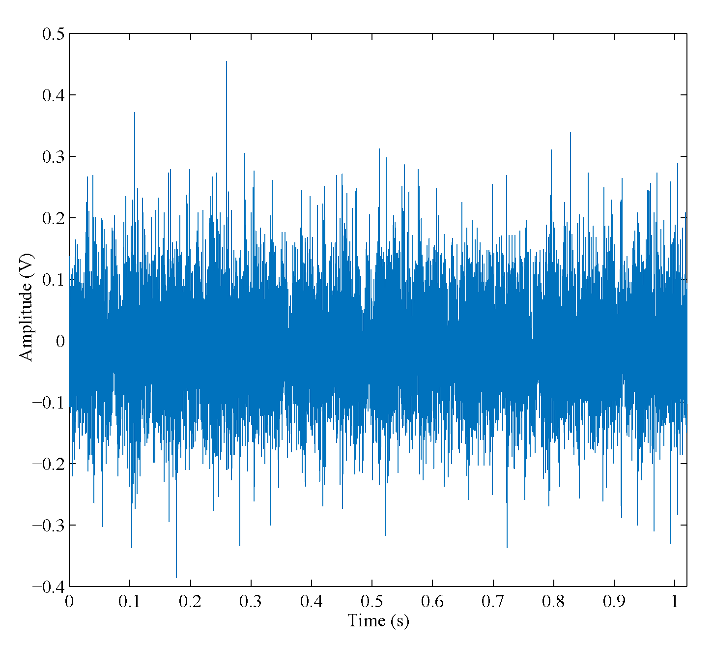
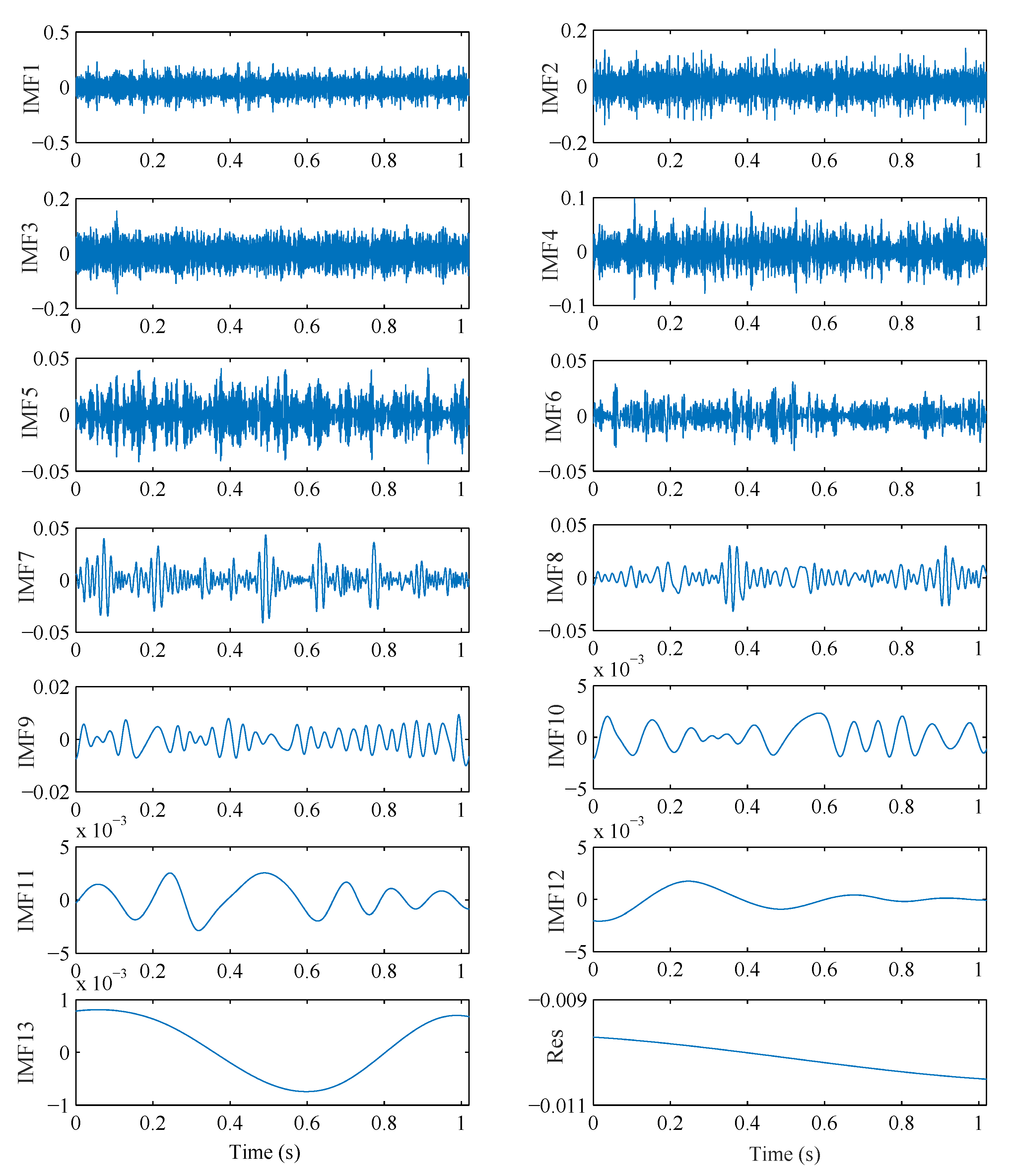
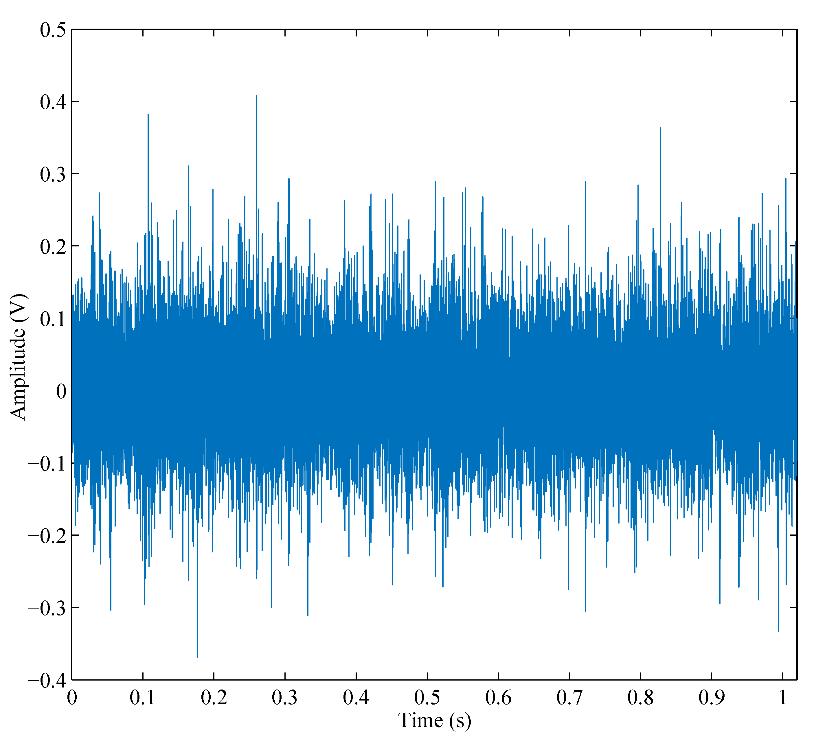
Figure 4 shows the original signals of the first data file, and all IMFs achieved by CEEMDAN are shown in Figure 5. With the definition of the threshold γ , the IMF with MIC value larger than γ is selected as the eligible one. For the first data file, Table 1 shows the MIC values of all IMFs achieved by CEEMDAN. The averaged MIC value between the original signals X and the random vector Ω is M X , Ω = 0.0479 ; thus, the threshold is set to γ = 1.5 × 0.0479 = 0.07185 .
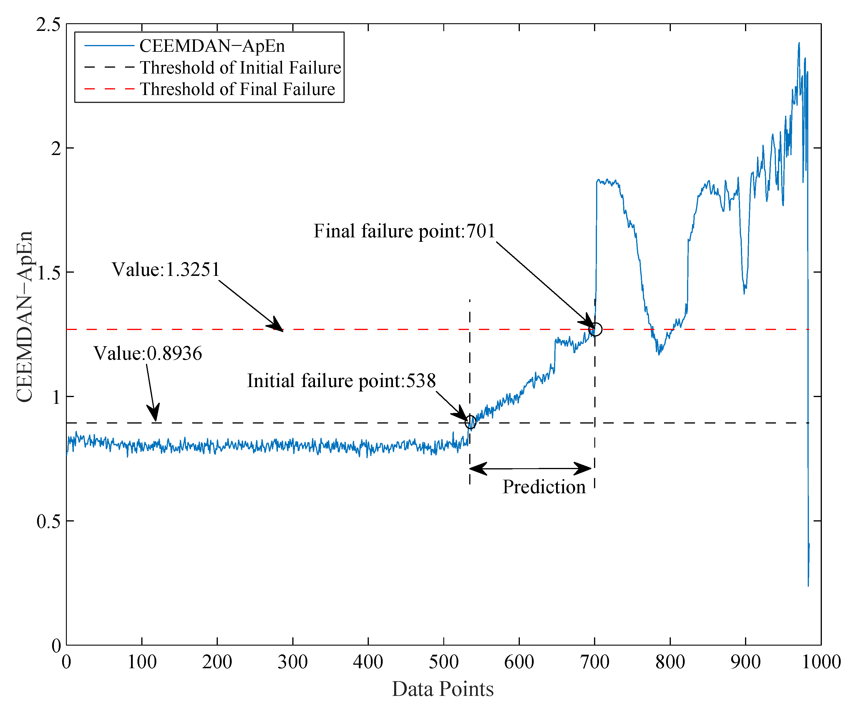
As shown in Table 1, IMFs numbered as 1, 2, 3, and 4 are selected to reconstruct the signals because their MIC values are greater than γ . Figure 6 shows the reconstructed signals with eligible IMFs. Then, the approximate entropy (ApEn) of the reconstructed signals is calculated as the health indicator of the rotating machinery. In other words, CEEMDAN-ApEn is the new proposed feature for failure prediction. Figure 7 shows the degradation curve based on the proposed CEEMDAN-ApEn feature.
As shown in Figure 7, the degradation curve is smooth at the initial period, which means the bearing is in normal condition. With the continuous growth of the running time of the bearing, the curve shows an upward trend, which means the gradual degradation of performance. At the final period, sharp fluctuation of the curve represents that the bearing appears a failure, and that is the end of the bearing. In summary, the proposed CEEMDAN-ApEn feature can reveal the entire life cycle of the bearing.
To describe the degradation process of the rotating machinery accurately, an effective feature should satisfy the following three conditions [35,36].
(1)
The feature should vary with degradation process gradually, thus maintaining a certain correlation with time.
(2)
The feature should show a consistent increasing or decreasing characteristics throughout the life cycle.
(3)
The feature should be robust to outliers.
Therefore, correlation, monotonicity and robustness are three metrics used to evaluate the performance of the proposed feature. Among them, the correlation metric is adopted to measure the correlation strength between the feature sequence and the time series, the monotonicity metric can describe the apparent degree of the feature sequence’s continuous increasing or decreasing, and the robustness metric is used to reveal the feature sequence’s tolerance to noise interference or abnormal signals.
Suppose E = e 1 , e 2 , , e K is the feature sequence, and T = t 1 , t 2 , , t K is a time series. e t k represents the feature value at time t k , and K represents the total time length. The feature sequence is divided into two parts by the moving average method as follows.
e t k = e T t k + e R t k ,
where e T t k is the stationary trend part, and e R t k is the random margin part. The correlation between E and T is remarked as C o r r E , T , the monotonicity and robustness of E is marked as M o n E and R o b E , respectively.
C o r r E , T = K k e T k t k K k e T k t k k t k K k e T k 2 k e T k 2 K k t k 2 k t k 2 ,
M o n E = 1 K 1 k δ e T k + 1 e T k k δ e T k e T k + 1 ,
R o b E = 1 K k exp e R k e k ,
where δ is a simple unit step function, which can be expressed as follows.
δ x = 1 , x 0 0 , x < 0 .
It is obvious that above three metrics vary in the interval [0,1]. However, a single metric can only measure certain aspect of the feature for failure prediction. To test the performance of the proposed feature comprehensively, a weighted combination metric should be constructed to fuse above three metrics, which is specifically expressed as:
J = ω 1 C o r r E , T + ω 2 M o n E + ω 3 R o b E s . t . = ω i > 0 i ω i = 1 , i = 1 , 2 , 3 ,
where ω i represents the importance weight of i-th metric. Because the monotonic trend has the greatest impact on the results of the RUL prediction, the importance weights are thus set to 0.2, 0.5, and 0.3 for correlation, monotonic, and robustness, respectively [35,36].
To illustrate the performance of the proposed feature, a comparison between other features (Kurtosis, RMS, ENTR [19], ApEn, and EEMD-EMTR [20]) and the proposed CEEMDAN-ApEn feature is carried out, and the results are shown in Table 2. As it shown, all above features can achieve good performance on robustness because their values are close to 1. Among them, RMS and the proposed CEEMDAN-ApEn features outperform others, which means they are robust to outliers. Furthermore, RMS achieves the best performance on monotonicity because it adopts an average strategy to reduce the random errors. It is worth mentioning that the proposed CEEMDAN-ApEn feature has a higher value on monotonicity; thus, it is applicable for continuous degradation tracking of the bearing. It is remarkable that the proposed CEEMDAN-ApEn feature achieves the best performance on correlation. Therefore, it can be utilized to perform RUL prediction of the bearing. In summary, the proposed CEEMDAN-ApEn feature has the highest value on the weighted combination metric, which means it can keep excellent balance among all influence factors of the failure prediction.

3.3. Initial and Final Failure Prediction

During the entire life cycle, the bearing will degrade continuously over time, and gradually changes from the healthy state to the failure state over a long period of time. Therefore, the threshold of the initial failure should be set to achieve the prediction starting time, and the threshold of the finial failure should also be set to end the prediction process.
As shown in Figure 7, the threshold of the initial failure is set as 0.8963 by using the Chebyshev inequality described in Section 2.3, and the degradation process starts from the 538th point, which is also named as PST. It is obvious that the degradation curve has a significantly sudden-changing at the 701st data point; thus, it is used as the final failure point, and the corresponding CEEMDAN-ApEn value (1.3251) is set as the threshold of the final failure.

3.4. RUL Prediction

The RUL prediction of the bearing starts from PST and ends at the data point where the value of the CEEMDAN-ApEn feature exceeds the threshold of the final failure for the first time. To illustrate the good performance of the proposed AR-UKF model, AR-PF model is also constructed. With the combination of AR model and particle filtering (PF) algorithm, AR-PF model has been adopted to resolve RUL prediction problem in many fields [19,37,38,39,40].
At the very beginning, a number of n = 40 data points from 538 to 577 is adopted to set up the AR model, and UKF is used to perform RUL prediction of the bearing as described in Figure 2. Because the predicted value of the CEEMDAN-ApEn feature exceeds the threshold of the final failure (1.3251) at the 124th data point, the predicted RUL at data point 578 is thus 1240 min (124 × 10 min) because the interval between neighbor data points is 10 min.
By repeating above process at each data point, a RUL curve can be achieved as shown in Figure 8, wherein the horizontal ordinate represents current time for prediction, and the vertical ordinate represents the corresponding real and predicted RUL. Obviously, the predicted RUL values of the proposed AR-UKF can follow the developing trend of the real RUL values accurately. By contrast, the predicted RUL values of the AR-PF model are more fluctuate, which means the uncertainty of prediction results.
To quantify the performance of the proposed AR-UKF model, results about the predicted RUL are assessed by the average error (AE) and root-mean-square error (RMSE), which are expressed as follows.
A E = 1 N i = 1 N R U L p i R U L r i ,
R M S E = 1 N i = 1 N R U L p i R U L r i 2 ,
where R U L p and R U L r are the predicted and the real RUL values, respectively, and N is the number of predicted points. The results are listed in Table 3.
As shown in Table 3, it is obvious that the values of AE and RMSE of the proposed AR-UKF model are less than that of the AR-PF model. Therefore, the proposed AR-UKF model can achieve RUL prediction task of the bearing accurately.

4. Conclusions

To resolve failure prediction problem of the rotating machinery, a novel method was developed in this paper. Because CEEMDAN not only can overcome the mode mixing effect of EMD but also should be able to avoid the decomposition errors caused by white noise in EEMD and CEEMD, it was applied to the original vibration signals to get a series of IMFs, and all eligible IMFs were selected by MIC to reconstruct the signals with helpful information. A feature named CEEMDAN-ApEn was proposed to describe the entire degradation process of the rotating machinery. Compared with existing features in this field, the new proposed CEEMDAN-ApEn feature can maintain an good balance among all influence factors of failure prediction. An efficient RUL prediction model by the combination of the AR model and UKF was developed to obtain the RUL of the rotating machinery. The experimental results show that the proposed method is beneficial and suitable for failure prediction of the rotating machinery.
It should be noted that the threshold of the final failure is an important parameter for the proposed failure prediction method, and now it is selected according to the practice and experience. Considering the diversity of the rotating machinery, future work will be devoted to select the appropriate value of this parameter adaptively. Moreover, the proposed method will be applied to real cases study concerning the failure prediction of the rotating automaton.

Author Contributions

Conceptualization, J.Y.; Formal analysis, Y.C.; Funding acquisition, J.Y.; Methodology, J.Y.; Project administration, J.W.; Resources, T.G.; Software, T.G.; Supervision, J.Y.; Validation, J.W.; Visualization, Y.C.; Writing—original draft, Y.C.; Writing—review & editing, T.G. All authors have read and agreed to the published version of the manuscript.

Acknowledgments

The authors would like to thank the editors and the reviewers for their helpful comments.

Conflicts of Interest

The authors declare no conflict of interest.

References

  1. Zhong, Q.; Zhang, Z. Several issues of scientific development of safety production (Including safety manufacturing) in China. Chin. J. Mech. Eng. 2007, 43, 7–18. [Google Scholar] [CrossRef]
  2. Li, X.; Zhang, Y. Development of fault detection and diagnosis technology of rolling bearing. Eng. Test 2009, 49, 1–5. [Google Scholar]
  3. Huang, Z. Historical review and future expectation of dimensionless diagnosis in China. China Plant Eng. 2000, 10, 30–35. [Google Scholar]
  4. Pan, Q.; He, T. Fault diagnosis of gears based on local mean decomposition combing with kurtosis. J. Vibroeng. 2014, 16, 2639–2648. [Google Scholar]
  5. Qiu, H.; Lee, J. Robust performance degradation assessment methods for enhanced rolling element bearings prognostics. Adv. Eng. Inform. 2003, 17, 127–140. [Google Scholar] [CrossRef]
  6. Heng, R.; Nor, M. Statistical analysis of sound and vibration signals for monitoring rolling element bearing condition. Appl. Acoust. 1998, 53, 211–226. [Google Scholar] [CrossRef]
  7. Li, Y.; Lin, J. A review on empirical mode decomposition in fault diagnosis of rotating machinery. Mech. Syst. Signal Process. 2013, 35, 108–126. [Google Scholar] [CrossRef]
  8. Dong, H.; Qi, K.; Chen, X. Shifting process of EMD and its application in rolling element bearing fault diagnosis. J. Mech. Sci. Technol. 2009, 23, 2000–2007. [Google Scholar] [CrossRef]
  9. Wang, J.; Gao, X.; Yan, R. Integration of EEMD and ICA for wind turbine gearbox diagnosis. Wing Energy 2014, 17, 757–773. [Google Scholar] [CrossRef]
  10. Zhao, X.; Patel, T.H.; Zuo, M.J. Multivariate EMD and full spectrum based condition monitoring for rotating machinery. Mech. Syst. Signal Process. 2012, 27, 712–728. [Google Scholar] [CrossRef]
  11. Yan, R.; Gao, R.X.; Chen, X. Wavelets for fault diagnosis of rotary machines: A review with applications. Signal Process. 2014, 96, 1–15. [Google Scholar] [CrossRef]
  12. Yan, R.; Gao, R.X. Multi-scale enveloping spectrogram for vibration analysis in bearing defect diagnosis. Neural Comput. 2009, 42, 293–302. [Google Scholar] [CrossRef]
  13. Wang, C.; Yan, R.; Gao, R. Unified time-scale-frequency analysis for machine defect signature extraction: Theoretical framework. Mech. Syst. Signal Process. 2009, 23, 226–235. [Google Scholar] [CrossRef]
  14. Yan, R.; Gao, R.X. An efficient approach to machine health evaluation based on harmonic wavelet packet transform. Robot. Comput. Integr. Manuf. 2005, 21, 291–301. [Google Scholar] [CrossRef]
  15. Chen, H.; Chen, X.; Zi, Y. An effective approach to rolling bearing diagnosis based on adaptive redundant second-generation wavelet. Int. J. Mater. Prod. Technol. 2008, 33, 65–78. [Google Scholar] [CrossRef]
  16. Dong, S.J.; Wu, W.L. Rolling bearing performance degradation assessment based on improved convolutional neural network with anti-interference. Measurement 2020, 151, 107219. [Google Scholar] [CrossRef]
  17. Zhao, X.L.; Jia, M.P. A new local-global deep neural network and its application in rotating machinery fault diagnosis. Neurocomputing 2019, 366, 215–233. [Google Scholar] [CrossRef]
  18. Wu, C.; Feng, F.; Wu, S.; Jiang, P.; Wang, J. A method for constructing rolling bearing lifetime health indicator based on multi-scale convolutional neural networks. J. Braz. Soc. Mech. Sci. Eng. 2019, 41, 526. [Google Scholar] [CrossRef]
  19. Qian, Y.; Yan, R. Remaining useful life prediction of mechanical rotary components using an enhanced particle filter. IEEE Trans. Instrum. Meas. 2015, 64, 2696–2707. [Google Scholar] [CrossRef]
  20. Rai, A.; Upadhyay, S.H. An integrated approach to bearing prognostics based on EEMD-multi feature extraction, Gaussian mixture models and Jensen-Renyi divergence. Appl. Soft Comput. 2018, 71, 36–50. [Google Scholar] [CrossRef]
  21. Chen, C.; Zhang, B.; Vachtsevanos, G. Prediction of machine health condition using neuro-fuzzy and Bayesian algorithms. IEEE Trans. Instrum. Meas. 2012, 61, 297–306. [Google Scholar] [CrossRef]
  22. Donga, M.; He, D. A segmental hidden semi-Markov model (HSMMS)-based diagnostics and prognostics framework and methodology. Mech. Syst. Signal Process. 2007, 21, 2248–2266. [Google Scholar] [CrossRef]
  23. Liao, L. Discovering prognostic features using genetic programming in remaining useful life prediction. IEEE Trans. Ind. Electron. 2014, 61, 2464–2472. [Google Scholar] [CrossRef]
  24. Oppenheimer, C.H.; Loparo, K.A. Physically based diagnosis and prognosis of cracked rotor shafts. In Proceedings of the SPIE—The International Society for Optical Engineering, Orlando, FL, USA, 24–27 July 2002; pp. 122–132. [Google Scholar]
  25. Qian, Y.; Yan, R.; Hu, S. Bearing degradation evaluation using recurrence quantification analysis and Kalman filter. IEEE Trans. Instrum. Meas. 2014, 63, 2599–2610. [Google Scholar] [CrossRef]
  26. Swanson, D.C.; Spencer, J.M.; Arzoumanian, S.H. Prognostic modelling of crack growth in a tensioned steel band. Mech. Syst. Signal Process. 2000, 14, 789–803. [Google Scholar] [CrossRef]
  27. Chen, X.; Shen, Z.; He, Z.; Sun, C.; Liu, Z. Remaining life prognostics of rolling bearing based on relative features and multivariable support vector machine. J. Mech. Eng. Sci. 2013, 227, 2849–2860. [Google Scholar] [CrossRef]
  28. Bustos, A.; Rubio, H.; Castejón, C.; García-Prada, J.C. EMD-Based methodology for the identification of a high-speed train running in a gear operating state. Sensors 2018, 18, 793. [Google Scholar] [CrossRef] [Green Version]
  29. Bustos, A.; Rubio, H.; Castejón, C.; García-Prada, J.C. Condition monitoring of critical mechanical elements through graphical representation of state configurations and chromogram of bands of frequency. Measurement 2019, 135, 71–82. [Google Scholar] [CrossRef]
  30. Torres, A.; Colominas, M.; Schlotthauer, G.; Flandrin, P. A complete ensemble empirical mode decomposition with adaptive noise. In Proceedings of the IEEE International Conference on Acoustics, Speech, and Signal Processing, Prague, Czech Republic, 22–27 May 2011; pp. 4144–4147. [Google Scholar]
  31. Reshef, D.N.; Reshef, Y.A.; Finucane, H.K.; Grossman, S.R.; McVean, G.; Turnbaugh, P.J.; Lander, E.S.; Mitzenmacher, M.; Sabeti, P.C. Detecting novel associations in large data sets. Science 2011, 334, 1518–1524. [Google Scholar] [CrossRef] [Green Version]
  32. Pincus, S.M. Approximate entropy as a measure of system-complexity. Proc. Natl. Acad. Sci. USA 1991, 88, 2297–2301. [Google Scholar] [CrossRef] [Green Version]
  33. Yu, J. Health condition monitoring of machines based on hidden Markov model and contribution analysis. IEEE Trans. Instrum. Meas. 2012, 61, 2200–2211. [Google Scholar] [CrossRef]
  34. Qian, Y.; Yan, R.; Gao, R.X. A multi-time scale approach to remaining useful life prediction in rolling bearing. Mech. Syst. Signal Process. 2017, 83, 549–567. [Google Scholar] [CrossRef] [Green Version]
  35. Zhang, B.; Zhang, L.J.; Xu, J.X. Degradation feature selection for remaining useful life prediction of rolling element bearings. Qual. Reliab. Eng. Int. 2016, 32, 547–554. [Google Scholar] [CrossRef]
  36. Camci, F.; Medjaher, K. Features evaluation for effective bearing prognostics. Qual. Reliab. Eng. Int. 2013, 29, 477–486. [Google Scholar] [CrossRef] [Green Version]
  37. Orchard, M.E.; Vachtsevanos, G.J. A particle-filtering approach for on-line fault diagnosis and failure prognosis. Trans. Inst. Meas. Control 2009, 31, 221–246. [Google Scholar] [CrossRef]
  38. Rigatos, G.G. Particle filtering for state estimation in nonlinear industrial systems. IEEE Trans. Instrum. Meas. 2009, 58, 3885–3900. [Google Scholar] [CrossRef]
  39. Chen, C.; Vachtsevanos, G.; Orchard, M.E. Machine remaining useful life prediction: An integrated adaptive neuro-fuzzy and highorder particle filtering approach. Mech. Syst. Signal Process. 2012, 28, 597–607. [Google Scholar] [CrossRef]
  40. Zhao, W.; Tao, T.; Ding, Z.; Zio, E. A dynamic particle filter-support vector regression method for reliability prediction. Reliab. Eng. Syst. Saf. 2013, 119, 109–116. [Google Scholar]
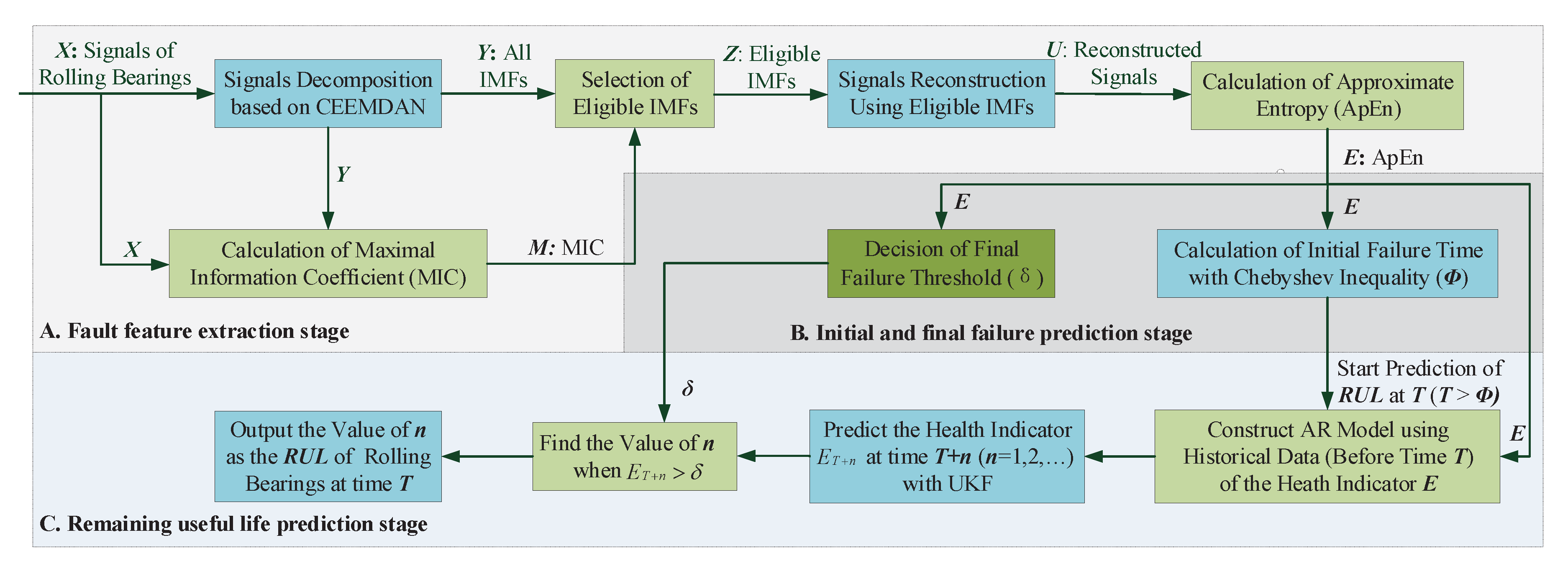
Figure 1. Functional block diagram of the proposed method. CEEMDAN = complete ensemble empirical mode decomposition with adaptive noise; IMFs = intrinsic mode functions; ApEn = approximate entropy; UKF = unscented Kalman filter; RUL = remaining useful life.
Applsci 10 02056 g001
Figure 2. The flow diagram of RUL prediction based on Autoregressive (AR)-UKF model. PST = prediction starting time.
Applsci 10 02056 g002
Figure 3. Bearing test-to-failure experiment system.
Applsci 10 02056 g003
Figure 4. The original signals of the first data file.
Applsci 10 02056 g004
Figure 5. IMFs of the original signals achieved by CEEMDAN.
Applsci 10 02056 g005
Figure 6. The reconstructed signals with eligible IMFs.
Applsci 10 02056 g006
Figure 7. The degradation curve based on CEEMDAN-ApEn.
Applsci 10 02056 g007
Figure 8. The RUL prediction curve of different models.
Applsci 10 02056 g008
Table 1. The MIC values of IMFs.
IMFs1234567
MIC0.29390.16430.17670.09870.05740.05020.0576
IMFs8910111213
MIC0.06100.05140.05350.05870.06880.0685
Table 2. The performance of all kinds of features. RMS = root mean square.
Features C o r r F , T M o n F R o b F J
Kurtosis0.55890.03560.95730.4221
RMS0.65960.09450.98370.4743
EEMD-EMTR0.72660.01930.97480.4474
ENTR0.74310.00510.83150.4006
ApEn0.75090.02340.96660.4518
CEEMDAN-ApEn0.83210.06410.98020.4925
Table 3. Quantitively evaluation results of different models. PF = particle filtering.
MetricsAR-PFAR-UKF
A E (unit: hour)0.22400.0093
R M S E (unit: hour)0.29590.0394