Abstract
Bearing failure generates impulses when the rolling elements pass the cracked surface of the bearing. Over the past decade, acoustic emission (AE) techniques have been used to detect bearing failures operated in low-rotating speeds. However, since the high sampling rates of the AE signals make it difficult to design and extract discriminative fault features, deep neural network-based approaches have been proposed in several recent studies. This paper proposes a convolutional neural network (CNN)-based bearing fault diagnosis technique. In this work, the normalized bearing characteristic component (NBCC) is used as the input of CNN, which is an effective form of representing bearing failure symptoms. In addition, importance-weight is extracted using gradient-weighted class activation mapping (Grad-CAM) for visual explanation of CNN. In the experiment result, the proposed approach achieves high classification accuracy with reasonable visualization, which shows that CNN successfully learned the components of bearing characteristic frequency for each type of bearing failure.
1. Introduction
Bearings are vital components of heavy rotating machines that reduce friction between a rotating shaft and fixed components such as bearing housings. It is known that 45–55% of failures of rotating machines are caused by bearing faults [1]. Hence, it is important to detect the arising bearing faults at the early stages to prevent the secondary failure of the manufacturing equipment. In the past decades, many bearing fault diagnosis techniques have been developed based on acoustic emission (AE). AE is the process of the generation of transient elastic waves from sudden cyclic fatigue, fraction, impacting, etc. [2,3,4,5]. Regarding bearings, the acoustic waves can be generated when the rolling elements of the bearing hit the cracked surface on the inner race, outer race, and rolling element. The advantage of AE-based analysis is its capability of detecting very low-energy signals caused by bearing failures at an early-stage or during slow-speed operation [2]. However, since the sampling rate used for AE signal collection is usually higher than 1 MHz, it is difficult to analyze the AE signal because of the tremendous amounts of data in the collected time-series (due to high signal sampling rates) and computational time required for analysis. Model-based feature extraction is one of promising approaches to overcome these issues because it converts big raw data instances into small feature vectors. Multipoint optimal minimum entropy deconvolution adjusted (MOMEDA) is introduced to extract informative features in several papers [6,7,8]. In these studies, the MOMEDA has been utilized to extract the fault period impulse component as features, which is the demodulated signal. Other papers developed deep neural network (DNN)-based bearing fault diagnosis methods [9,10,11,12,13,14]. DNN-based bearing diagnosis methods are powerful tools to extract informative features by learning feature representations from a large amount of raw data. Recently, some papers compared the performance of convolutional neural network (CNN) and DNN-based approaches. From these papers we could conclude that the CNN-based techniques are much better than DNN-based methods in terms of fault diagnosis performance [3,12,15,16]. Although DNN or CNN-based methods have achieved high classification accuracy, there are still two issues that must be resolved to make these methods highly applicable to real applications. The first issue is that the trained neural network, in general, can be only reliable on the specific machine since the patterns of the raw signals strongly depend on the operating conditions of the machinery such as load, installation, external vibration, etc. The second concern is that the trained feature representation is uninterpretable due to the black box-like operation of the neural networks.
This paper proposes a new CNN-based rolling element bearing fault diagnosis approach to resolve the aforementioned problems. To address the first issue, the proposed method utilizes the normalized bearing characteristic components (NBCC) as the input data of CNN rather than raw AE signal itself. Since the bearing characteristic frequencies are induced by appearing bearing failures, NBCC is a more effective representation for diagnosing the bearing failure symptoms. To resolve the second issue, this paper applies the gradient-weighted class activation mapping (Grad-CAM) to visualize important regions in NBCC. According to the literature, Grad-CAM is a promising method that provides visual explanations of the classification result of a CNN in object detection and recognition [17].
The remainder of this paper is organized as follows. Section 2 introduces the proposed methodology for diagnosing rolling element bearing faults using AE signals. In Section 3 the bearing fault simulator used for collecting AE signals is presented. The fault diagnosis results demonstrated and discussed in Section 4. Finally, Section 5 contains the concluding remarks.
2. Proposed Method
Figure 1 illustrates the process of diagnosing bearing faults by the proposed method as a flowchart. In step 1, the envelope power spectra are calculated from pre-acquired AE signals containing healthy and faulty conditions. In step 2, frequency magnitudes are extracted from the characteristic frequency range of the bearing and used as features. In step 3, the CNN is trained using the extracted features. Here, the envelope power spectra of new AE signals are classified into healthy or faulty condition using the trained CNN. Finally, in step 4, the importance weights with frequency are generated including valuable regions in the envelope spectrum using Grad-CAM for the acquired AE signals.

Figure 1.
Flowchart of the proposed approach.
2.1. Envelope Analysis
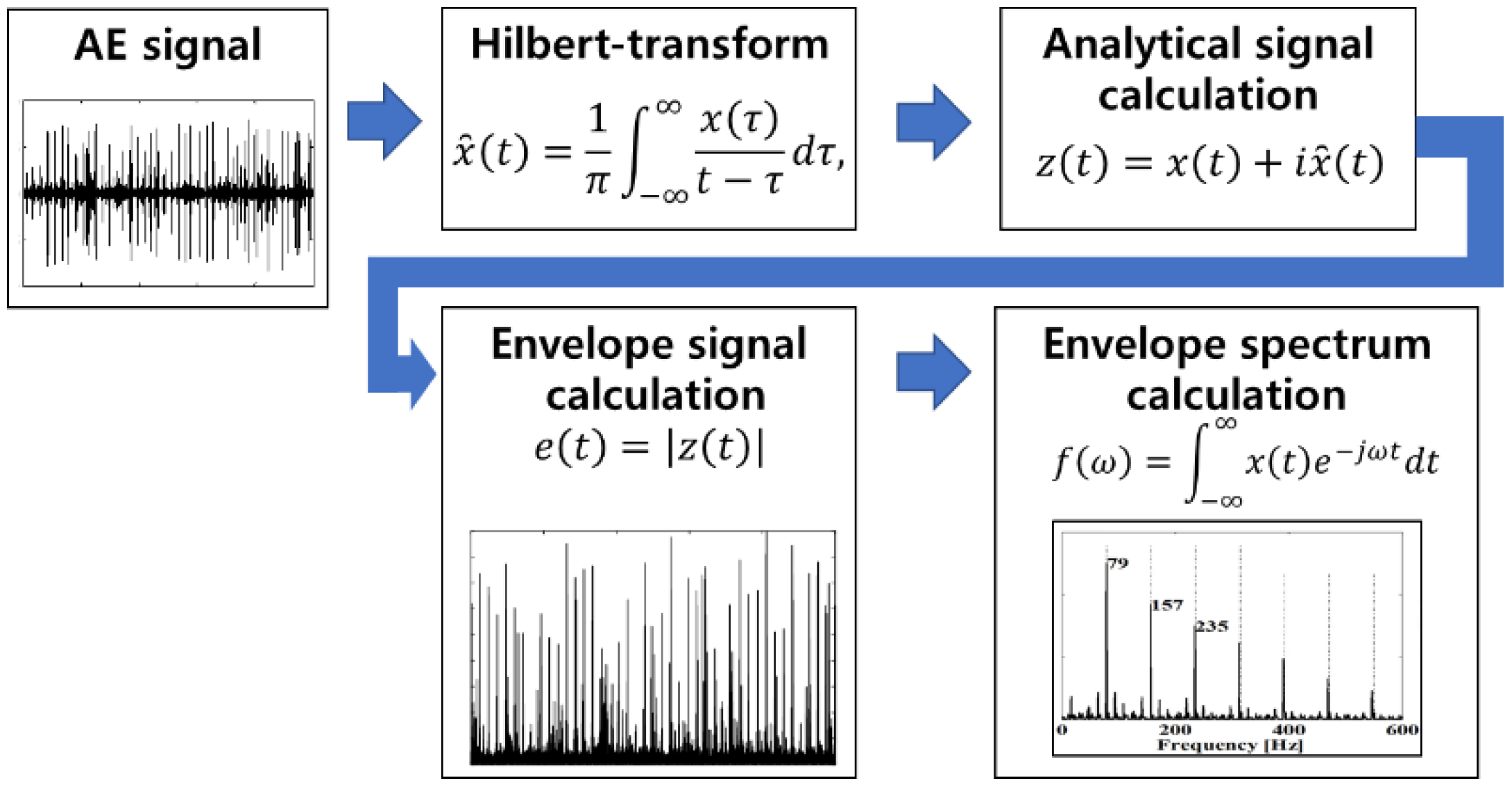
Since the impulses generated by bearing failures are amplitude-modulated, AE signals should be first demodulated to extract pure burst signals. As shown in Figure 2, the Hilbert-transform-based envelope analysis was used to demodulate the AE signal [18,19]. First, the Hilbert-transform was applied to the AE signal as follows [18]:
where t is the time, is a sample of the input signal at , and is a sample of the Hilbert-transformed signal at time t. Hilbert-transform shifts the phase of the input signal by 90 degrees.
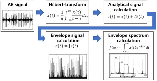
Figure 2.
The flowchart of the envelope analysis. Hilbert-transform is applied to the acoustic emission (AE) signal to calculate the 90-degree phase-shifted signal. Then, the analytical signal is calculated by sum of the original signal and its Hilbert-transform as an imaginary number. Next, the envelope signal is calculated by applying absolute operation to the previously computed analytical signal. Finally, the fast Fourier transform of the envelope signal provides an envelope spectrum.
To obtain the analytical signal, z(t), the Hilbert-transformed signal, , and input signal, x(t) were combined as complex numbers [18]:
Then, the envelope signal, e(t) was computed as . Finally, the envelope spectrum, f() was calculated as the square root of the fast Fourier transform of e(t) as follows:
2.2. Bearing Characteristic Component Analysis
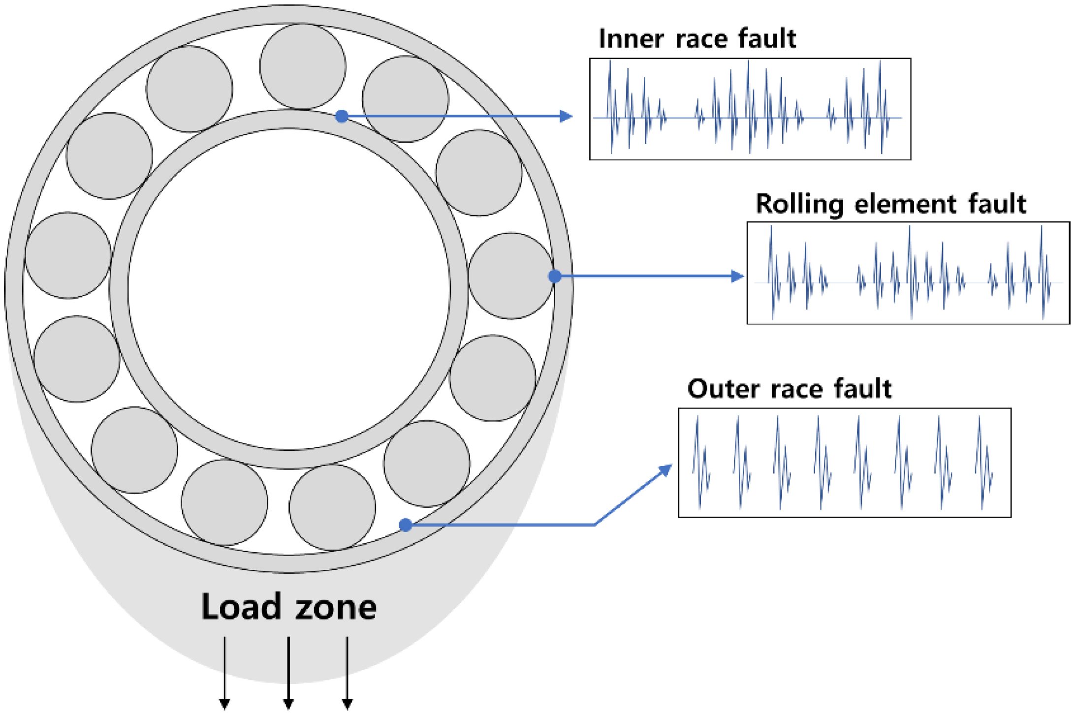
Bearing failures generate periodic burst signals that are represented as the bearing characteristic frequency harmonics in the spectrum [20]. The outer race way with a crack on its surface (ORCS) emits a periodic pulse each time when the rolling element passes over the cracked surface. Since the outer race is a static component of the bearing and the applied load to cracked surface is always stable, the amplitude of the impulses does not change. The inner race way with a crack on its surface (IRCS) generates a series of impulses when each rolling element hits the crack on the inner race of the bearing. By rotating the inner ring with the shaft, the response of impulses grows up periodically when the inner race passes loaded zone, which is oriented to the direction of gravity. Since this phenomenon modulates the impulses by rotating speed, the sideband of rotating speed appears nearby the characteristic frequency of inner race. The rolling element with a crack on its surface (RECS) generates impulses by hitting inner and outer races. The magnitude of the impulse is affected by whether the contact occurred in the loaded or unloaded zones. Similarly, the sideband of RECS is a fundamental train frequency [20]. Figure 3 illustrates the examples of the ideal signals for ORCS, IRCS, and RECS.

Figure 3.
Examples of the ideal signals for each type of bearing fault.
Accordingly, the bearing characteristic (or defect) frequencies are categorized into ball pass frequency on the outer race (BPFO), ball pass frequency on the inner race, (BPFI), and ball spin frequency (BSF). BPFO, BPFI, and 2×BSF are caused by the bearing failures of the outer race, inner race, and rolling element, respectively. The bearing characteristic frequencies are defined as follows [20]:
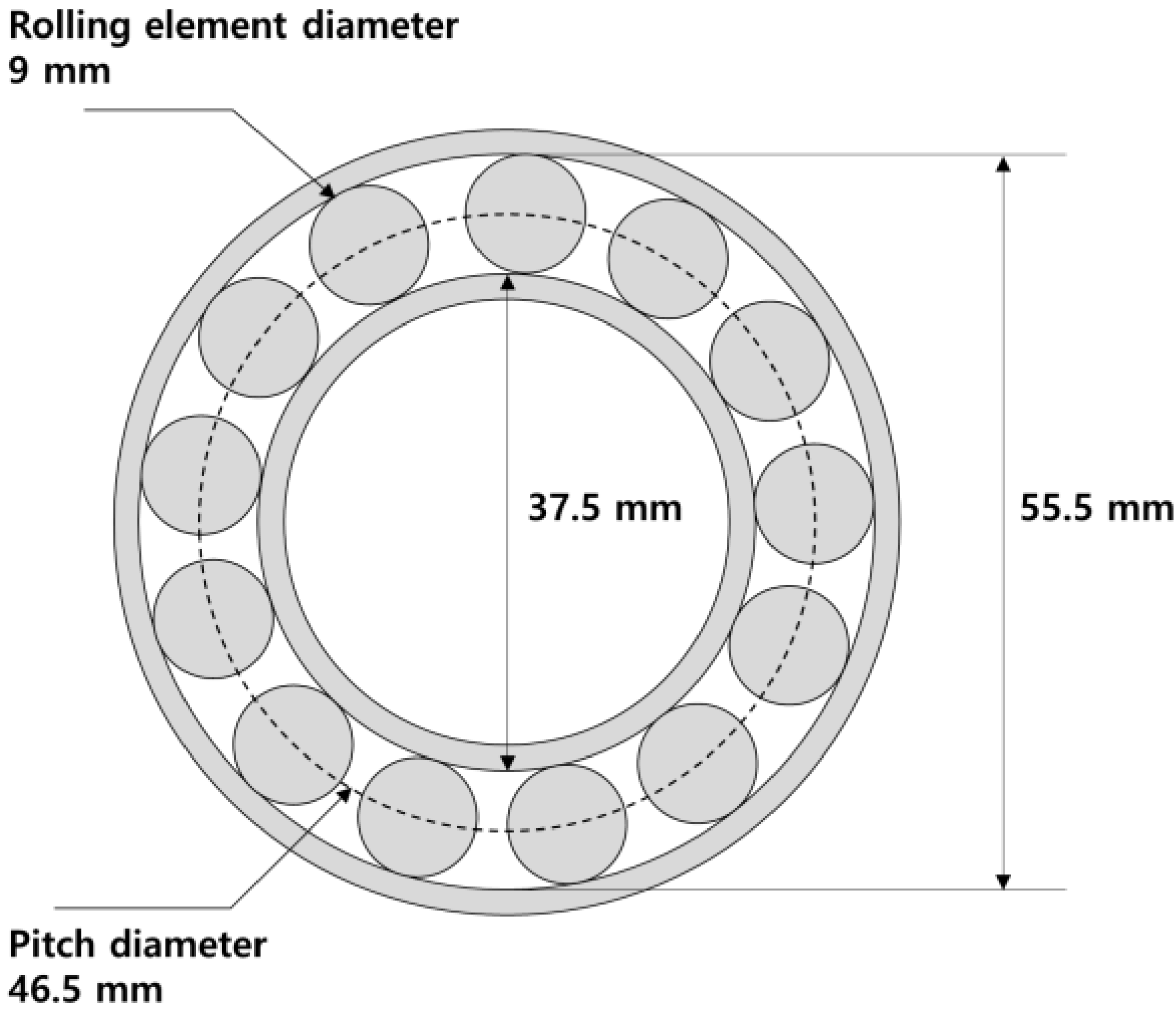
where Nb is the number of rolling elements, S is the shaft speed, Bd is the diameter of the rolling element, Pd is the pitch diameter, i.e., the distance between the center of a rolling element and the center of the inner race, and θ is a contact angle of the rolling element with respect to the shaft.
The bearing characteristic components (BCCs) were extracted as an input vector of the CNN. BCCs are defined as follows:
where f are the values of the envelope spectrum and Fmax is the frequency, which is higher than all the harmonics of bearing characteristic frequencies as below:
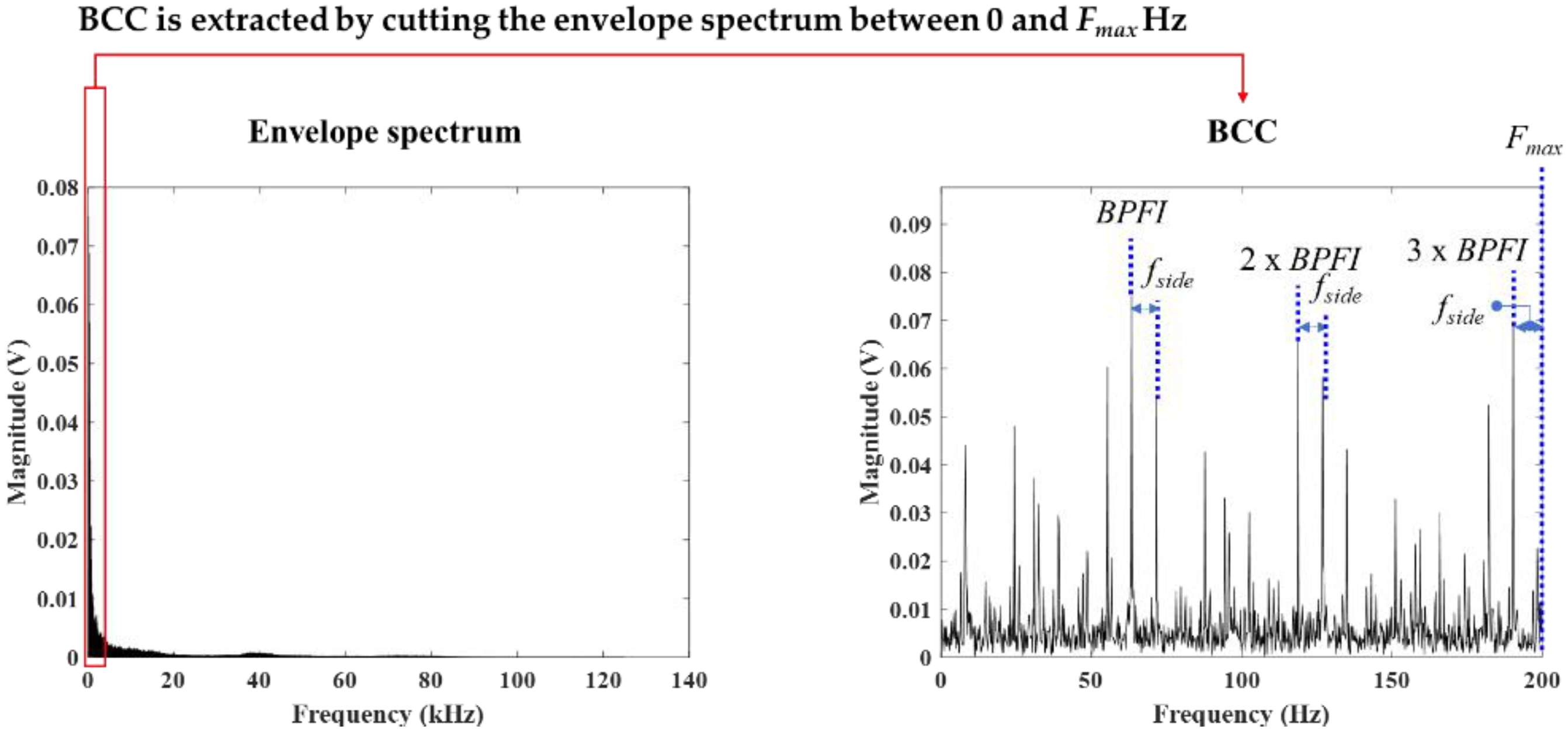
where n is the number of frequency harmonics and fside is the sideband of the highest characteristic frequency. Table 1 shows fside for each type of bearing characteristic frequency. In this paper, Fmax was equal to BPFI, which is the highest among the bearing characteristic frequencies. Figure 4 depicts the extraction process of BCCs.

Table 1.
The specification of the target bearing, FAG NJ206-E-TVP2.
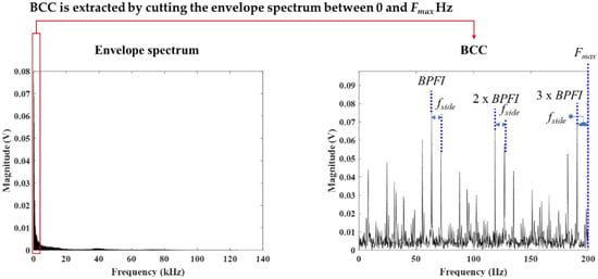
Figure 4.
The extraction process of bearing characteristic components.
Since the variation of magnitude makes the training CNN unstable, BCCs are min–max normalized to be used for input data of CNN as follows:
2.3. Training and Classification
The structure of CNN is represented in Figure 5. The proposed CNN had six convolutional layers and two fully connected (FC) layers. Each convolutional layer consisted of a one-dimensional (1-D) convolutional layer, a batch-normalization layer, and a rectified linear unit (ReLU). All convolutional layers were connected to each other using a max pooling layer with a down-sampling factor of 2. The input size of each convolutional layer was half of the input size of the previous convolutional layer, except for the first layer. The FC layers and softmax role classification were the last layers [21]. For the training process, multiclass categorical cross-entropy was used as the loss function, and the Adam optimization algorithm was used for backpropagation [22].
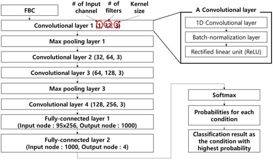
Figure 5.
Convolutional neural network (CNN) structure for bearing fault diagnosis.
2.4. Importance-Weight Extraction
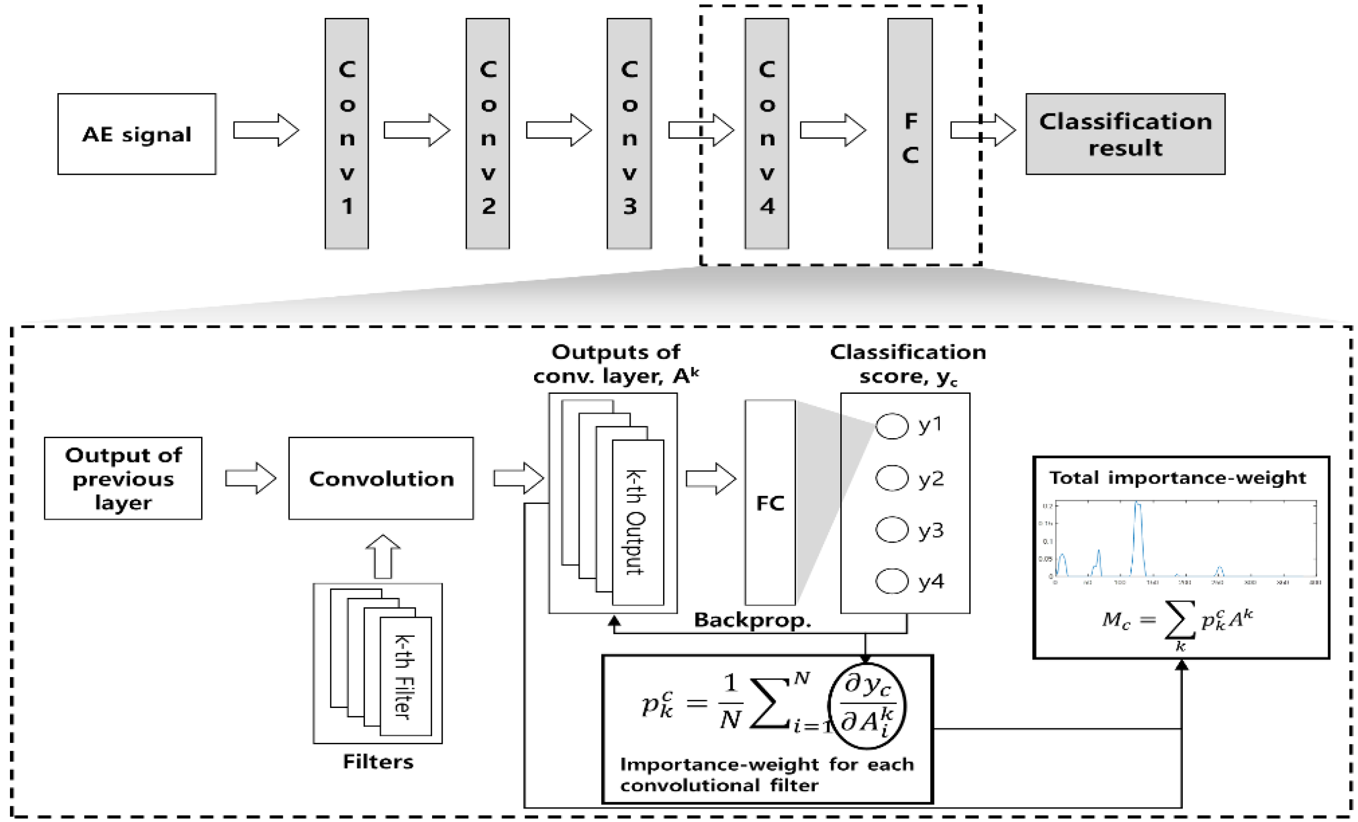
Figure 6 illustrates the flowchart of Grad-CAM with an example of CNN structure. Each convolutional layer consisted of several filters with trainable filter coefficients. CNN applies these filters to the input data for extracting the informative features from the data. In Grad-CAM, the outputs of final convolutional layers were used to calculate the importance-weight for each characteristic frequency in NBCC. To obtain the importance-weight, a partial derivative of the score for class c was calculated of the k-th activation map. The following equation represents the definition of [17]:
where pkc indicates the importance-weight of the k-th filter for class c, yc is a classification score of class c, and is i-th element in k-th activation map. When CNN was being trained, was calculated in the back-propagation step. Finally, the importance-weight of class c was calculated as follows [17]:
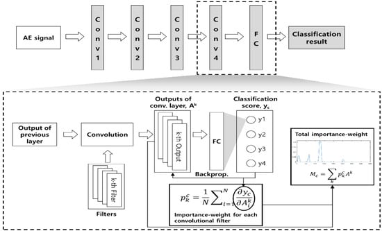
Figure 6.
The flowchart of gradient-weighted class activation mapping (Grad-CAM) with an example of the CNN structure.
3. Experimental Setup and Data Acquisition
To validate the proposed method, a bearing fault simulator was used for measuring healthy and faulty-state AE signals of the rolling element bearing. The established bearing fault simulator is illustrated in Figure 7. On the drive-end shaft, a three-phase induction motor was connected to a gearbox by flexible coupling. The gearbox transferred the torque of the induction motor to the non-drive-end shaft with a gear reduction ratio of 1.52:1. A tachometer was installed to measure the rotating speed of the non-drive-end shaft. A cylindrical roller bearing (FAG NJ206-E-TVP2), which was the target bearing of the experiment, was installed in the bearing housing of the non-drive-end shaft. To apply radial and axial load, a fan with adjustable blades was connected to the non-drive-end shaft via a belt. The shaft speed was 500 revolutions per minute (RPM) in this paper. An AE sensor was attached on the bearing housing of the target bearing. The measurement device for obtaining AE signals was a PCI-2-based system. A general-purpose wideband AE sensor, whose frequency response was between 100 and 1000 kHz, was used to capture resonance frequency signals containing modulated bearing signals.
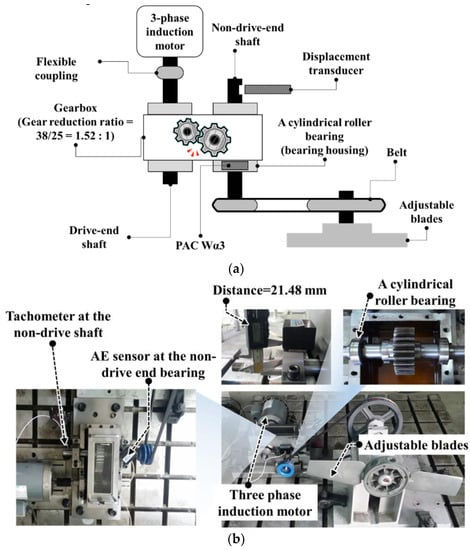
Figure 7.
The illustration of the bearing fault simulator: (a) the diagram of the bearing fault simulator and (b) the photographs of the bearing fault simulator.
Figure 8 and Table 2 shows the specification of the target bearing. The contact angle was 0 because the target bearing was a radial bearing. By using Equations (4)–(6) with the bearing parameters and shaft speed, the bearing characteristic frequencies of BPFO, BPFI, and BSF were equal to 43.68 Hz, 20.72 Hz, and 64.65 Hz, respectively.

Figure 8.
Illustration of the bearing, FAG NJ206-E-TVP2.

Table 2.
The specification of the target bearing, FAG NJ206-E-TVP2.
The seeded bearing faults, which are the outer race way with a crack on its surface (ORCS), inner race way with a crack on its surface (IRCS), and rolling element with a crack on its surface (RECS), are shown in Figure 9. The crack dimension of the bearing failures was 6 mm × 0.5 mm × 0.5 mm. In addition, Figure 10 illustrates an example of the AE signals for each bearing condition in the dataset. As shown in Figure 10, the healthy bearing (HB) contained less impulses than the ones in faulty conditions. On the contrary, the signal of bearing faults such as ORCS, IRCS, and RECS emitted more impulses created by the cyclic impacts of faults.

Figure 9.
The seeded bearing faults: (a) outer race way with a crack on its surface (ORCS); (b) inner race way with a crack on its surface (IRCS); and (c) rolling element with a crack on its surface (RECS).

Figure 10.
The examples of AE signals for each bearing conditions listed as: (a) the AE signal of the healthy bearing; (b) the AE signal of ORCS; (c) the AE signal of IRCS; and (d) the AE signal of RECS.
4. Experimental Results and Discussion
To validate the performance of Grad-CAM for the bearing fault diagnosis, AE signals from the healthy-state and three types of bearing fault were acquired using the testbed. The length of a measured AE signal was 1 second with a 1 MHz sampling rate and the number of AE signals for each condition was 600. Half of the data instances from the collected dataset were randomly selected for training the CNN. The remaining unseen samples were used for validating the fault diagnosis capabilities of the trained CNN. The trained CNN achieved 99% classification accuracy on the validation dataset, as shown in the confusion matrix depicted in Figure 11.
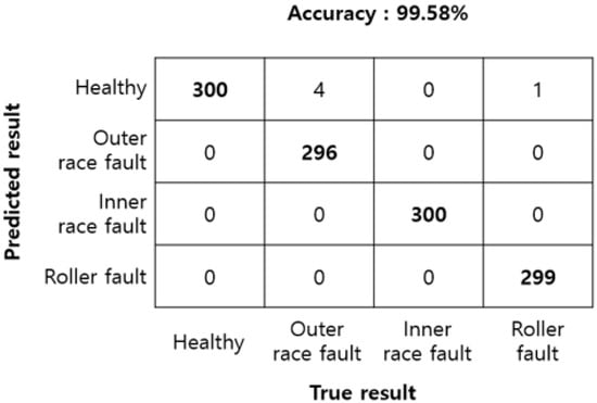
Figure 11.
Confusion matrix of the classification result.
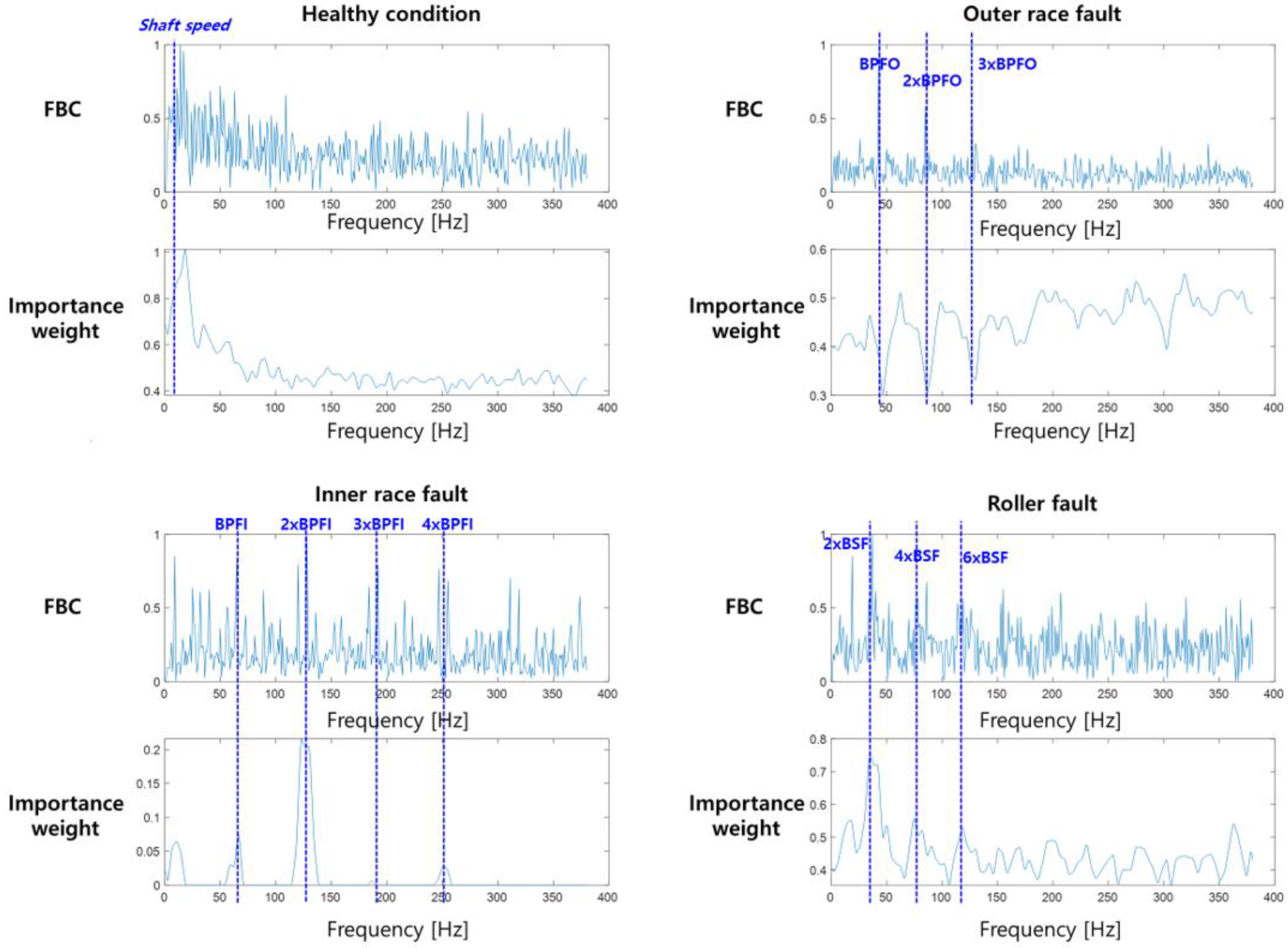
Figure 12 demonstrates the importance-weight over frequency component of the envelope spectrum. As shown in the figure, the CNN learned that the harmonics of defect frequencies were important information for classifying the states of the bearing. In this study, BPFO, BPFI, BSF, and the shaft speed were 44, 42, 65, and 8.33 Hz, respectively. For the healthy condition, CNN learned that low frequency band components were important since the low frequency band contained the harmonics of the shaft speed frequency that could be clearly observed in the healthy condition of the bearing. Since the defect and shaft speed frequencies are also valuable in traditional bearing fault diagnosis methods, it seems that the CNN was trained without any fault-related information. In the case of outer race fault, the values of 2×BSF and BPFO harmonics were too similar that made it difficult to classify the input data based on these characteristic frequencies. Therefore, the CNN chose the sideband of BPFO as useful information instead of BPFO, itself.
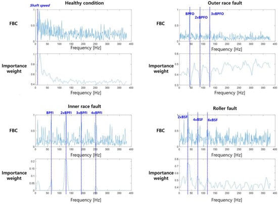
Figure 12.
Importance-weights for each bearing failure.
5. Conclusions
In this paper, we proposed NBCC, which contains bearing characteristic frequencies for training CNNs when used for the task of rolling element bearing fault diagnosis. In addition, we analyzed the feature representation of the trained CNN for the bearing fault diagnosis using the Grad-CAM technique. In the experiment, a custom simulator was used to imitate bearing faults. Using the bearing fault simulator, AE signals were measured for healthy state of the bearing and three different types of bearing faults such as the outer race way, inner race way, and rolling element with a crack on their surface. In the experimental result, the CNN achieved 99% accuracy when trained with the proposed NBCC. The result also demonstrated that the low frequency components were important for classifying healthy state of the bearing, whereas bearing characteristic frequencies were essential for diagnosing various types of bearing faults. This result indicates that CNN trained with the proposed NBCC properly understood the valuable features of the envelop power spectrum for each bearing condition used in this work. For the application of CNNs in real environment, the proposed approach can be utilized to verify whether CNN learns inappropriate feature representation or not.
Author Contributions
All of the authors contributed equally to the conception of the idea, the design of experiments, the analysis and interpretation of results, as well as the writing of the manuscript. Writing—original draft preparation, J.K. and J.-M.K.; writing—review and editing, J.K. and J.-M.K. All authors have read and agreed to the published version of the manuscript.
Funding
This work was supported by the Korea Institute of Energy Technology Evaluation and Planning (KETEP) and the Ministry of Trade, Industry and Energy (MOTIE) of the Republic of Korea (No. 20181510102160). This work was also supported by the Technology Infrastructure Program funded by the Ministry of SMEs and Startups (MSS, Korea).
Conflicts of Interest
The authors declare no conflict of interest.
Nomenclature
The following nomenclatures are used in this manuscript
| k-th output of a convolutional layer | |
| BCC | bearing characteristic components |
| the diameter of the rolling element of bearing | |
| BPFO | ball pass frequency on the outer race of bearing |
| BPFI | ball pass frequency on the inner race of bearing |
| BSF | ball spin frequency of bearing |
| a sample of envelope signal at the time, t | |
| the maximum frequency covering bearing characteristic frequencies and harmonics | |
| the magnitude of envelope spectrum at the frequency, | |
| The sideband of bearing characteristic frequency | |
| the importance-weight for the input data, | |
| the number of harmonics of bearing characteristic frequencies used in the proposed method | |
| the number of rolling elements | |
| normalized bearing characteristic components | |
| importance weight vector of k-th filter of a convolutional layer for class, c | |
| the pitch diameter of rolling element bearing | |
| shaft rotating speed | |
| a sample of signal at the time, t | |
| a sample of Hilbert-transformed signal at time, t | |
| the score of classification for class, c | |
| a sample of analytical signal at the time, t | |
| the contact angle of rolling element |
References
- Nandi, S.; Toliyat, H.A.; Li, X. Condition Monitoring and Fault Diagnosis of Electrical Motors—A Review. IEEE Trans. Energy Convers. 2005, 20, 719–729. [Google Scholar] [CrossRef]
- Elforjani, M.; Mba, D. Accelerated natural fault diagnosis in slow speed bearings with Acoustic Emission. Eng. Fract. Mech. 2010, 77, 112–127. [Google Scholar] [CrossRef]
- Tra, V.; Khan, S.A.; Kim, J.-M. Diagnosis of bearing defects under variable speed conditions using energy distribution maps of acoustic emission spectra and convolutional neural networks. J. Acoust. Soc. Am. 2018, 144, EL322–EL327. [Google Scholar] [CrossRef]
- Prosvirin, A.; Kim, J.; Kim, J.-M. Bearing Fault Diagnosis Based on Convolutional Neural Networks with Kurtogram Representation of Acoustic Emission Signals. In Advances in Computer Science and Ubiquitous Computing; Park, J.J., Loia, V., Yi, G., Sung, Y., Eds.; Springer: Singapore, 2018; pp. 21–26. [Google Scholar]
- Islam, M.R.; Uddin, J.; Kim, J.-M. Acoustic emission sensor network based fault diagnosis of induction motors using a gabor filter and multiclass support vector machines. Ad Hoc Sens. Wirel. Netw. 2016, 34, 273–287. [Google Scholar]
- Sun, H.; Wu, C.; Liang, X.; Zeng, Q. Identification of Multiple Faults in Gearbox Based on Multipoint Optional Minimum Entropy Deconvolution Adjusted and Permutation Entropy. Entropy 2018, 20, 850. [Google Scholar] [CrossRef]
- Li, Z.; Ma, J.; Wang, X.; Wu, J. MVMD-MOMEDA-TEO Model and Its Application in Feature Extraction for Rolling Bearings. Entropy 2019, 21, 331. [Google Scholar] [CrossRef]
- Cai, W.; Wang, Z. Application of an Improved Multipoint Optimal Minimum Entropy Deconvolution Adjusted for Gearbox Composite Fault Diagnosis. Sensors 2018, 18, 2861. [Google Scholar] [CrossRef] [PubMed]
- Wasmer, K.; Saeidi, F.; Meylan, B.; Le Quang, T.; Shevchik, S. When AE (Acoustic Emission) meets AI (Artificial Intelligence) II. In Proceedings of the EWGAE 2018, Senlis, France, 12–14 September 2018. [Google Scholar]
- Islam, M.M.M.; Kim, J.-M. Automated bearing fault diagnosis scheme using 2D representation of wavelet packet transform and deep convolutional neural network. Comput. Ind. 2019, 106, 142–153. [Google Scholar] [CrossRef]
- Hasan, M.J.; Islam, M.M.M.; Kim, J.-M. Acoustic spectral imaging and transfer learning for reliable bearing fault diagnosis under variable speed conditions. Measurement 2019, 138, 620–631. [Google Scholar] [CrossRef]
- Appana, D.K.; Prosvirin, A.; Kim, J.-M. Reliable fault diagnosis of bearings with varying rotational speeds using envelope spectrum and convolution neural networks. Soft Comput. 2018, 22, 6719–6729. [Google Scholar] [CrossRef]
- Tra, V.; Kim, J.; Kim, J.-M. Fault Diagnosis of Bearings with Variable Rotational Speeds Using Convolutional Neural Networks. In Advances in Computer Communication and Computational Sciences; Bhatia, S.K., Tiwari, S., Mishra, K.K., Trivedi, M.C., Eds.; Springer: Singapore, 2019; pp. 71–81. [Google Scholar]
- Duong, B.P.; Kim, J.-M. Fault Diagnosis of Multiple Combined Defects in Bearings Using a Stacked Denoising Autoencoder. In Advances in Computer Communication and Computational Sciences; Bhatia, S.K., Tiwari, S., Mishra, K.K., Trivedi, M.C., Eds.; Springer: Singapore, 2019; pp. 83–93. [Google Scholar]
- Tra, V.; Kim, J.; Khan, S.A.; Kim, J.-M. Bearing Fault Diagnosis under Variable Speed Using Convolutional Neural Networks and the Stochastic Diagonal Levenberg-Marquardt Algorithm. Sensors 2017, 17, 2834. [Google Scholar] [CrossRef] [PubMed]
- Appana, D.K.; Ahmad, W.; Kim, J.-M. Speed Invariant Bearing Fault Characterization Using Convolutional Neural Networks. In Multi-disciplinary Trends in Artificial Intelligence; Phon-Amnuaisuk, S., Ang, S.-P., Lee, S.-Y., Eds.; Springer International Publishing: Cham, Switzerland, 2017; pp. 189–198. [Google Scholar]
- Selvaraju, R.R.; Cogswell, M.; Das, A.; Vedantam, R.; Parikh, D.; Batra, D. Grad-CAM: Visual Explanations from Deep Networks via Gradient-based Localization. Int. J. Comput. Vis. 2020, 128, 336–359. [Google Scholar] [CrossRef]
- Wang, N.; Liu, X. Bearing Fault Diagnosis Method Based on Hilbert Envelope Demodulation Analysis. IOP Conf. Ser. Mater. Sci. Eng. 2018, 436, 012009. [Google Scholar]
- Kang, M.; Kim, J.; Wills, L.M.; Kim, J.-M. Time-Varying and Multiresolution Envelope Analysis and Discriminative Feature Analysis for Bearing Fault Diagnosis. IEEE Trans. Ind. Electron. 2015, 62, 7749–7761. [Google Scholar] [CrossRef]
- Randall, R.B.; Antoni, J. Rolling element bearing diagnostics—A tutorial. Mech. Syst. Signal Process. 2011, 25, 485–520. [Google Scholar] [CrossRef]
- Sainath, T.N.; Mohamed, A.; Kingsbury, B.; Ramabhadran, B. Deep convolutional neural networks for LVCSR. In Proceedings of the 2013 IEEE International Conference on Acoustics, Speech and Signal Processing, Vancouver, BC, Canada, 26–31 May 2013; pp. 8614–8618. [Google Scholar]
- Zhang, Z.; Sabuncu, M.R. Generalized cross entropy loss for training deep neural networks with noisy labels. In Proceedings of the the 32nd International Conference on Neural Information Processing Systems, Montréal, QC, Canada, 3–8 December2018; pp. 8792–8802. [Google Scholar]
© 2020 by the authors. Licensee MDPI, Basel, Switzerland. This article is an open access article distributed under the terms and conditions of the Creative Commons Attribution (CC BY) license (http://creativecommons.org/licenses/by/4.0/).


