Actuator Weak Fault Diagnosis in Autonomous Underwater Vehicle Based on Tri-Stable Stochastic Resonance

Abstract

The autonomous underwater vehicle (AUV) is mainly used in the development and exploration of the ocean. As an important module of the AUV, the actuator plays an important role in the normal execution of the AUV. Therefore, the fault diagnosis of the actuator is particularly important. At present, the research on the strong faults, such as the winding of the actuator, has achieved good results, but the research on the weak fault diagnosis is relatively rare. In this paper, the tri-stable stochastic resonance model is analyzed, and the ant colony tri-stable stochastic resonance model is used to diagnose the weak fault. The system accurately diagnoses the fault of the actuator collision and verifies the adaptive tri-stable stochastic resonance system. This model has better diagnostic results than the bi-stable stochastic resonance system.

1. Introduction

An autonomous underwater vehicle (AUV) usually performs various tasks in the complex marine environment, but the occurrence of failure will cause a loss that cannot be measured. Therefore, there is a need for an intelligent vehicle capable of responding to an emergency; that is, it should be able to perform automatic fault diagnosis [1].

The AUV consists of several components, of which the actuator is the key component and the most heavily loaded component. In the marine environment, there are external random disturbances, such as currents and strong measurement noise. AUV itself is a strong nonlinear system with large inertia and large time-delay characteristics, which makes the theory and method of the actuator fault diagnosis. Many scholars have made research results in AUV actuator fault diagnosis technology, but most of them focus on the hard faults of the actuator and the large loss of output, but less on the weak fault diagnosis. At the same time, the weak faults of the actuators are mostly early faults. Effective detection and diagnosis of early faults as early as possible plays an important role in avoiding “catastrophic accidents” caused by AUVs [2,3,4].

The main problems of fault diagnosis for AUV actuators are: Santosa et al. [5] established an AUV fault diagnosis model with four horizontal and two vertical thrusters. The methodology defines that, in the case of partial fault or complete fault (failure) in horizontal thrusters located in different action planes (which defines the axis or plane where component(s) of forces are actuating in this plane), horizontal propelling forces are calculated through the allocation matrix, used in the pseudo-inverse method, without any change, and a modified weighted matrix. Alvarez et al. [6] presented how the model is learned using the Expectation Maximization algorithm for Gaussian Mixtures and how the testbed is monitored by probabilistic inference. The jamming fault of the motor and other faults are simulated and diagnosed by using a GMM classifier through the motor temperature, current, voltage, and other data. They described how the framework deals with non-Gaussian data and how it reflects in the accuracy overall.

Sun et al. [7] introduced an improved Elman neural network, which was applied to the underwater vehicle motion modeling. Through designing a self-feedback connection with fixed gain in the unit connection, as well as increasing the feedback of the output layer node, the improved Elman network has faster convergence speed and generalization ability. This method for a high-order nonlinear system has stronger identification ability. Zhang et al. [8] improved the multi-fault pattern classifier training speed and fault diagnosis accuracy of the fuzzy weighted support vector domain description (FWSVDD), and a multi-fault mode classification method based on a hierarchical strategy was proposed. A model-based fault diagnosis method was established on the Livingstone 2 system, and a fault tree was established to classify faults by level [9].

The main problems of weak fault diagnosis for AUV actuators are: Nascimento et al. [10] presented an evaluation of Recurrent Neural Networks (RNN) for a data-driven fault detection and diagnosis scheme for underwater thrusters with empirical data. The nominal behavior of the thruster was modeled using the measured control input, voltage, rotational speed, and current signals. They evaluated the performance of fault classification using all the measured signals compared to using the computed residuals from the nominal model as features.

Partial kernel principal component analysis (PKPCA) was studied for sensor fault detection and isolation (FDI) of an autonomous underwater vehicle. In order to achieve fault isolation, partial KPCA was proposed where a set of residual signals was generated based on the parity relation concept.

And by building models of actuators or systems, researchers have used a data-driven approach [11], Gaussian Particle Filter [12], Terminal Sliding Mode Observer [13], Non-Linear Principal Component Analysis (NLPCA) Hybrid Approach [14], and Gaussians and Variational Bayes Approximation (Fagogenis et al.).

The weak faults of actuators are usually early faults. If these early weak faults of actuators can be detected as early as possible, the strong faults of actuators that will eventually stop working will be avoided. The AUV can make a corresponding judgment and treatment in time to avoid the occurrence of greater accidents. It can be seen from the above literature that the current fault diagnosis has a good effect on the diagnosis of strong faults, and most of them adopt the method of fault data training and actuator models. Therefore, the method in this paper can adaptively diagnose weak faults without fault data and a system model [15,16].

The second section is the related theory of the Tri-stable stochastic resonance fault diagnosis, which is introduced from (1) the AUV actuator dynamics model. (2) Principle of stochastic resonance. (3) Parameter compensation stochastic resonance. (4) Ant colony optimization algorithm principle. The third section is influencing factors of a multi-stationary stochastic resonance system. The fourth section is a practical engineering application. The fifth section presents conclusions.

2. Tri-Stable Stochastic Resonance Theory

2.1. AUV Actuator Dynamics Model

The omnidirectional actuator spindle speed control part controls the permanent magnet synchronous motor to rotate according to the speed of the main control unit, and then drives the omnidirectional actuator main shaft to rotate, thereby bringing the actuator to rotate. The spindle speed control part is composed of a power amplifier, a system controller, a permanent magnet synchronous motor, a signal detecting device, and a speed reducer. The spindle speed control composition diagram is shown in Figure 1. The motor driver, permanent magnet synchronous motor, drive board, power supply, etc., are built up to form the system.

When the omnidirectional actuator pitch angle is used for periodic motion, it will generate six directions of motion, which will change the speed and actuator of the actuator load of the submersible. If the omnidirectional actuator is moving at a uniform speed, the forces in all directions will balance forces to keep the speed stable. However, when the force of the omnidirectional actuator changes, the force of each fire blade will be uneven, causing the change of the spindle speed and direction. The mathematical model of the spindle speed control system is established by considering various factors. The equation of motion of the spindle system is obtained by the momentum moment theorem

$$2\pi I\frac{dn}{dt}=M_E-M_P-M_f,$$

(1)

$$m\frac{d{V}_s}{dt}=T-R,$$

(2)

In the Formula (1): $M_E$ is the driving torque of the motor, $M_P$ is the resistance torque of the blade, T is the effective thrust of the actuator, $M_f$ is the friction torque of the propeller, I is the moment of inertia of the propulsion motor, and $\frac{dn}{dt}$ is the rotation speed change rate. In Equation (2): m is the mass of the submersible, $\frac{d{V}_s}{dt}$ is the rate of change of the speed of the omnidirectional actuator, R is the hull resistance. Obtained by the momentum moment theorem

$$M_E=9.55\frac{P_e}{n_e},$$

(3)

$$M_P=K_Q\rho n^2{d}_p^5,$$

(4)

Among them, $d_p$ is the actuator diameter, $\rho$ is the seawater density, $P_e$ is the power of the drive motor, n is the propeller speed, and $n_e$ is the motor speed. In Formula (1), the moment of inertia I of the main propulsion motor is equal to the sum of the motor, the actuator shaft, and the blade to the moment of inertia of the submerged main propulsion system.

$$I=I_{motor}+I_{shaft}+I_{blade},$$

(5)

Among them, $I_{shaft}$ is the moment of inertia of the actuator shaft, $I_{motor}$ is the moment of inertia of the internal rotating part of the propulsion motor, $I_{blade}$ is the moment of inertia of the actuator. In the actuator design, if there is no detailed design information, it can be utilized. The empirical formula is calculated

$$I_{blade}=\frac{1}{4}{k}_1{k}_2{k}_3{k}_4\gamma \theta \frac{t_0{d}_p^4}{g},$$

(6)

where $k_2$ is the blade section parameter, $k_3$ is the blade shape coefficient, and these two coefficients can be selected according to the actual situation, $k_4$ is the blade clamp ratio coefficient, $k_1$ is the paddle coefficient, which can be taken as 1.025–1.06, $\gamma$ is the paddle Density, $\theta$ is the width ratio of the paddle, $t_0$ is the blade root thickness at the axis, and $d_p$ is the paddle tip thickness, g is the gravitational acceleration. Finding the $I_{blade}$ from Equation (6) requires a detailed understanding of the geometry of the actuator. If the detailed set parameters of the actuator are not available, an empirical formula can be used to estimate

$$I_{blade}=\frac{W}{g}{\left(\frac{k{d}_p}{2}\right)}^2,$$

(7)

where k is the coefficient, $k=0.4$, and W is the weight of the full paddle. $P_e$ is the power of the drive motor, n actuator speed, $n_e$ is the motor speed. When the voltage is constant, we use the current as the fault diagnosis parameter.

2.2. Principle of Stochastic Resonance

So far, with the continuous exploration of the stochastic resonance (SR) field, the multi-stable SR has attracted wide attention from scholars. It is well known that the nonlinear Langevin equation explains the principle of stochastic resonance from the perspective of Brownian particle motion. Therefore, this section generalizes the equation to a multi-stable system and briefly describes the effects of random forces on the system [17].

2.2.1. Langevin Equation

In order to describe the motion law of Brownian particles in liquid, the dynamic equation of Brownian particles is given, and on this basis, the Langevin Equation is established. The macroscopic equation for the motion of a Brownian particle of mass in a liquid is

$$m\dot{v}=-\alpha v,$$

(8)

Among them, v is the velocity of movement of the Brownian particles in the liquid, and $-\alpha v$ is the viscous force. When the mass of the Brownian particles is large, in addition to the macroscopic viscous force, the Brownian particles are also subjected to random motion in all directions by the force of the liquid molecules. The smaller the mass of the Brownian particles, the greater the magnitude of the motion, so we add the force $F\left(t\right)$ of the molecular clutter to Equation (8).

$$mv=-\alpha v+F\left(t\right),$$

(9)

where $F\left(t\right)$ is the total force generated by the collision of liquid molecules with Brownian particles. By dividing both sides of Equation (9) by m, can get

$$\dot{v}+\gamma v=\mathsf{\Gamma }\left(t\right),$$

(10)

And, $r=\frac{\alpha }{m}$, $\mathsf{\Gamma }\left(t\right)=\frac{F\left(t\right)}{m}$ is the damping coefficient per unit mass and the molecular collisional fluctuation force, $\mathsf{\Gamma }\left(t\right)$ is called Langevin force, and Formula (10). It is called the Langevin equation. Suppose that the particle $t=0$ has the velocity $v_0$ and the position is at $x_0$, then $v=\dot{x}$ is taken into Equation (10).

$$\ddot{x}+\gamma \dot{x}=\mathsf{\Gamma }\left(t\right),$$

(11)

Since the Brownian particles are still subjected to external forces, the Langevin equation under the action of the external field becomes

$$\ddot{x}+\gamma \dot{x}=f\left(x\right)+\mathsf{\Gamma }\left(t\right),$$

(12)

where $f\left(x\right)$ is the external force to which the average unit mass of Brownian particles is subjected. In the case of over-damping, the left side of Equation (12) is the damping term, which plays a major role, so the inertia term $\ddot{x}$ can be ignored, and $\gamma =1$, (12) can be reduced to

$$\dot{x}=f\left(x\right)+\mathsf{\Gamma }\left(t\right),$$

(13)

When the external force $f\left(x\right)$ of the average unit mass Brownian particle is a nonlinear multipotential function, the equation shown by Equation (13) is called the nonlinear Langevin equation [18,19,20].

2.2.2. Fokker–Planck Equation

The nonlinear Langevin equation has no fixed solution, so scholars turn to study the evolution of the Langevin equation. Let $\rho \left(x\right)$ be the distribution function of x, and its Markov process is described as

$$P(x_n,t_n|x_{n-1},t_{n-1};\dots ;x_1,t_1)=P(x_n,t_n|x_{n-1},t_{n-1}),$$

(14)

Its distribution function is

$$\rho (x,t+\tau )=\int P(x,t+\tau |x^{\prime },t)\rho (x^{\prime },t)d{x}^{\prime },$$

(15)

Expanding the above formula can get

$$\frac{\partial \rho (x,t)}{\partial t}=\left\{\sum _{n=1}^{\infty }{(-\frac{\partial }{\partial x})}^n\underset{\tau \to 0}{lim}\frac{M_n(x,t,\tau )}{n!\tau }\right\}\rho (x,t),$$

(16)

From Equation (16), to obtain the solution of the function $\rho (x,t)$, we need to know the transition moments $M_n(x,t,\tau )$ of each order. Equation (13) at $t+\tau$, the center distances of the centers centered on x are

$$M_n(x,t,\tau )=\langle {[x(t+\tau )-x]}^n\rangle ,$$

(17)

$$x(t+\tau )-x={\int }_t^{t+\tau }\left[f(x\left(t^{\prime }\right),t^{\prime })\right]d{t}^{\prime },$$

(18)

Substituting the above equation into Equation (16) yields the Fokker–Planck Equation (FPE) as

$$\frac{\partial \rho (x,t)}{\partial t}=-\frac{\partial }{\partial x}\left\{[f(x,t)+D\eta (x,t){\eta }^{\prime }(x,t)]\rho (x,t)\right\}+D\frac{{\partial }^2}{\partial x^2}\left[{\eta }^2(x,t)\rho (x,t)\right],$$

(19)

2.2.3. Multi-Stationary Stochastic Resonance Model

When the external force $f\left(x\right)=-U^{\prime }\left(x\right)$ of the particle in the nonlinear Langevin equation, $\mathsf{\Gamma }\left(t\right)=\xi \left(t\right)$ is taken into Equation (13)

$$\dot{x}=-U^{\prime }\left(x\right)+s\left(t\right)+\xi \left(t\right),$$

(20)

where $U\left(x\right)$ is a class of nonlinear polystable potential functions, as shown in (20). Among them, $a,b,c$ are the number of systems, and both are greater than 0.

$$U\left(x\right)=\frac{a}{2}{x}^2-\frac{1+a}{4b}{x}^4+\frac{c}{6}{x}^6,$$

(21)

Suppose the system input signal is $s\left(t\right)$ and Equation (21) is taken into Equation (20).

$$\dot{x}=-ax+\frac{1+a}{b}{x}^3-c{x}^5+s\left(t\right)+\xi \left(t\right),$$

(22)

where $s\left(t\right)$ is an input signal superimposed on multiple frequencies, representing an external force, as shown in Equation (23)

$$s\left(t\right)=\sum _{i=1}^n{A}_{i}sin\left(2\pi f_{i}t\right),i=1,2,\dots ,n,$$

(23)

In the formula, $A_i$ is the amplitude of the signal, $f_i$ is the frequency of the signal, and n is the number of input signals. Suppose that the statistical characteristics of $\xi \left(t\right)$ are shown in Equation (24), D is the noise intensity, and $t^{\prime }$ is the time delay of t.

$$\langle \xi \left(t\right)\rangle \ge 0,\langle \xi \left(t\right)\xi \left(t^{\prime }\right)\rangle \ge 2D\delta (t-t^{\prime }),$$

(24)

According to Formula (24) the Fourier expansion of $\xi \left(t\right)$ can obtain its power spectrum.

$$S\left(\omega \right)=\int e^{-i\omega \tau }2D\delta \left(\tau \right)d\tau =2D,$$

(25)

From Equation (25), the power spectrum $S\left(\omega \right)$ is independent of $\omega$, that is, the spectrum is a white spectrum. Therefore, the lang of Equation (24), in which the time correlation function is $\xi \left(t\right)$, is called white noise. At the same time, the nonlinear Langevin equation can be written as

$$\dot{x}=-ax+\frac{1+a}{b}{x}^3-c{x}^5+s\left(t\right)+D\xi \left(t\right),$$

(26)

The above formula is a kind of nonlinear Langevin equation with three steady-state points, which is essentially the periodic transition of the particle in the potential well of the nonlinear system under the action of all the forces.

In the multi-stable SR system described in Equation (26), when the system is in equilibrium, there are three steady-state solutions (minimum points) and two unsteady solutions (maximum points), respectively, Equations (27) and (28):

$$\left\{\begin{array}{c}-x_2=-\sqrt{\frac{1}{2c}(\frac{1+a}{b}+\sqrt{{\left(\frac{1+a}{b}\right)}^2-4ac})}\hfill \\ x_0=0\hfill \\ x_2=\sqrt{\frac{1}{2c}(\frac{1+a}{b}+\sqrt{{\left(\frac{1+a}{b}\right)}^2-4ac})}\hfill \end{array}\right.$$

(27)

$$\left\{\begin{array}{c}-x_1=-\sqrt{\frac{1}{2c}(\frac{1+a}{b}-\sqrt{{\left(\frac{1+a}{b}\right)}^2-4ac})}\hfill \\ x_1=\sqrt{\frac{1}{2c}(\frac{1+a}{b}-\sqrt{{\left(\frac{1+a}{b}\right)}^2-4ac})}\hfill \end{array}\right.$$

(28)

At this time, the corresponding intermediate well depth $\Delta U_M$ and the potential well depth $\Delta U_{L,R}$ are

$$\Delta U_M=\frac{1}{24c^2}\left[{\left({\left(\frac{1+a}{b}\right)}^2-4ac\right)}^{\frac{3}{2}}-\frac{1+a}{b}\left({\left(\frac{1+a}{b}\right)}^2-6ac\right)\right],$$

(29)

$$\Delta U_{L,R}=\frac{1}{12c^2}{\left[{\left(\frac{1+a}{b}\right)}^2-4ac\right]}^{\frac{3}{2}},$$

(30)

When $A_i=D=0,a=3,b=5,c=0.038$, the potential function curve of the multi-stable system is shown in Figure 2.

When $A_i=0;D\ne 0,$ that is, there is no periodic signal input and only the noise signal acts, the particles will randomly jump between the three potential wells of the multi-stable system without periodicity.

When $A_i\ne 0;D=0$, when there is only periodic signal input and no noise signal is excited, the equilibrium state of the system will change, and the three potential wells will generate periodic tilt with the same frequency under the action of the periodic signal. When the particle energy is less than the energy required to cross the barrier, the particle can only periodically move in the same potential of the input signal in one of the potential wells of the multi-stable system. The initial state of the particle is which potential well it is ultimately in; the decisive factor in doing periodic movements.

When $A_i\ne 0;D\ne 0$, that is, when the periodic signal and the noise signal are simultaneously excited, the inclination of the potential well in the multi-stable system will increase. In addition, the periodic signal also causes the potential well depth of the three potential wells of the multi-stable potential function to periodically change and can guide the noise signal to perform synchronous switching. When a certain matching relationship is achieved between the signal, the noise, and the multi-stable SR system, the particles can periodically transition between the potential wells, and the output signal of the system is in multiple potentials according to the frequency f of the input signal. The periodic transition is such that the component of the system output $x\left(t\right)$ that is of co-frequency with the input signal is enhanced [21,22,23].

2.3. Parameter Compensation Stochastic Resonance

With the in-depth study of SR theory by scholars, the problem that classical SR is limited by the adiabatic approximation theory is solved. At present, stochastic resonance can not only detect low frequency $(f<<1$ Hz) signals but also detect high frequency $(f>>1$ Hz) signals, and the signal frequency far exceeds the frequency range limited by traditional SR theory.

Existing methods for detecting high-frequency signals include subsampling, modulation, normalization, and parameter compensation. The principle of the subsampling method is simple and easy to operate, but the method has requirements on the sampling frequency and is difficult to determine. The modulation method theory is simple, but the method is very restrictive due to the difficulty in determining the frequency of the modulation signal. The normalized transform can convert the high frequency frequency domain to the low frequency frequency domain, but the method will greatly reduce the amplitude of the measured signal during processing, so the amplitude of the output signal of the system is smaller than the amplitude of the input signal. The parameter compensation method is to compensate for the influence of the frequency of the high-frequency signal to be tested on the amplitude of the output signal of the system. Therefore, it is only necessary to know the approximate range of the frequency of the signal to be detected during the detection, which is not only simple in principle and convenient in operation but also subject to very few restrictions. The literature has carried out a preliminary study on the parameter compensation SR, which proves the effectiveness of the method. The specific principles of using the parameter compensation SR are as follows:

The nonlinear multipotential function $U\left(x\right)=\frac{a}{2}{x}^2-\frac{1+a}{4b}{x}^4+\frac{c}{6}{x}^6$ and the input signal $s\left(t\right)$ Equation (23) are substituted by Equation (20) in the middle

$$\dot{x}=-ax+\frac{1+a}{b}{x}^3-c{x}^5+\sum _{i=1}^n{A}_{i}sin\left(2\pi f_{i}t\right)+D\xi \left(t\right),$$

(31)

By integrating Equation (31), the output signal x of the SR system is

$$\begin{array}{cc}\hfill x& =\int \left[-ax+\frac{1+a}{b}{x}^3-c{x}^5+\sum _{i=1}^n{A}_{i}sin\left(2\pi f_{i}t\right)+D\xi \left(t\right)\right]dt\hfill \\ \hfill & =\int \left[-ax+\frac{1+a}{b}{x}^3-c{x}^5\right]dt+\int \left[\sum _{i=1}^n{A}_{i}sin\left(2\pi f_{i}t\right)\right]dt+\int \left[D\xi \left(t\right)\right]dt\hfill \\ \hfill & =-\frac{a}{2}{x}^2+\frac{1+a}{4b}{x}^4-\frac{c}{6}{x}^6-\left[\sum _{i=1}^n\frac{A_i}{2\pi f_i}cos\left(2\pi f_{i}t\right)\right]+\int \left[D\xi \left(t\right)\right]dti=1,2,\cdots ,n\hfill \end{array}$$

(32)

As observed in Equation (32), the input signal $s\left(t\right)$ is processed by the multi-stable SR system, and its amplitude $A_i$ becomes $\frac{1}{2\pi f_i}$ of the original signal. When $f_i<<1$, then $\frac{1}{2\pi f_i}>1$ the amplitude $A_i$ of the input signal $s\left(t\right)$ is amplified; when $f_i>1$, then $\frac{1}{2\pi f_i}<1$, the input signal $s\left(t\right)$ value $A_i$ is reduced, and it can be found that as the input signal $s\left(t\right)$ frequency $f_i$ increases, the amplitude $A_i$ of the input signal x is greatly reduced. Therefore, high frequency signals cannot be seen in the output of the SR system excited by the high frequency signal. For this problem, the compensation parameter G can be added to cancel the signal amplitude $A_i$ reduction caused by the high frequency signal frequency $f_i$:

$$\begin{array}{cc}\hfill \dot{x}& =G\left[-ax+\frac{1+a}{b}{x}^3-c{x}^5+s\left(t\right)+D\xi \left(t\right)\right]\hfill \\ \hfill & =G\left[-ax+\frac{1+a}{b}{x}^3-c{x}^5+\sum _{i=1}^n{A}_{i}sin\left(2\pi f_{i}t\right)+D\xi \left(t\right)\right],\hfill \end{array}$$

(33)

In Equation (33), G is the compensation parameter. When the value of G is equal to $2\pi f_i$, the amplitude $A_i$ of the input signal $s\left(t\right)$ after passing through the SR system is unchanged. If the value of G is greater than $2\pi f_i$, the input signal is $s\left(t\right)$. After the SR system, the amplitude $A_i$ will be amplified, so in practice, G should be greater than $2\pi f_i$.

Let $\widehat{a}=Ga,\widehat{b}=\frac{G(1+a)}{b},\widehat{c}=Gc,\widehat{u}\left(t\right)=Gu\left(t\right)=G\left({\sum }_{i=1}^n{A}_{i}sin\left(2\pi f_{i}t\right)+D\xi \left(t\right)\right)$ substituting into Equation (26), we can get

$$\dot{x}=-\widehat{a}x+\widehat{b}{x}^3-c{x}^5+\widehat{u}\left(t\right),$$

(34)

2.4. Ant Colony Optimization Algorithm Principle

The ant colony algorithm is a population-based heuristic bionic evolution proposed by Italian scholar Colorni et al. In the early 1990s, by simulating the behavior of ants collectively, searching for the shortest path from food source to nest. The ant colony algorithm was first successfully applied to solve the famous traveling salesman problem (TSP), so it is explained by the classical symmetric TSP problem [24].

The TSP problem can be described as: Given cities, find the shortest path that passes through each city once and only once, and finally return back to the starting point. Let the number of ants in the ant colony be m; $d_{i,j}(i,j=1,2,\dots ,n)$ represents the distance between cities $i,j$; $b_i\left(t\right)$ represents the number of ants located in city i at time t, then $m={\sum }_{i=1}^n{b}_i\left(t\right)$; ${\tau }_{ij}\left(t\right)$ represents the pheromone concentration on the line $i,j$ at time t. At the initial time, the amount of information on each path is equal, and ${\tau }_{ij}\left(0\right)=C$ (C is a constant). The ant $k(k=1,2,\dots ,m)$ determines the direction of the transfer according to the amount of information on each path during the motion. At time t, the probability $p_{ij}^t$ of ant k moving from city i to city j is:

$$p_{ij}^k\left(t\right)=\left\{\begin{array}{c}\frac{{\tau }_{ij}^{\alpha }\left(t\right){\eta }_{ij}^{\beta }\left(t\right)}{{\sum }_{t\notin tab{u}_k}{\tau }_{ij}^{\alpha }\left(t\right){\eta }_{ij}^{\beta }\left(t\right)}j\notin tab{u}_k\hfill \\ 0otherwise\hfill \end{array}\right.$$

(35)

In the formula: ${\eta }_{ij}$—visibility, the heuristic information for the city i to transfer to the city j in the TSP problem; $\alpha$—the importance of residual information on the path; $\beta$—the importance of inspiring information; $tab{u}_k$—record the city that ant k is currently passing, called the taboo table, $tab{u}_k$ dynamically adjusted with the evolution process. After n moments, all ants complete an ant colony cycle, and the pheromone concentration on each edge is updated as follows.

$${\tau }_{ij}(t+n)=\rho {\tau }_{ij}t+\Delta {\tau }_{ij}t,$$

(36)

$$\Delta {\tau }_{ij}t=\sum _{k=1}^m\Delta {\tau }_{ij}^k,$$

(37)

In the formula: $\rho$—pheromone residual coefficient; $\Delta {\tau }_{ij}t$ and $\Delta {\tau }_{ij}^k$—ant colony and ant k in the time period t to $(t+n)$, the pheromone concentration left on the path $i,j$ is different according to the specific algorithm, the expression form of $\Delta {\tau }_{ij}^k$ is different. DorigoM has given three different computational models, called the ant-cycle algorithm, the ant-density algorithm, and the ant-quantity algorithm. The fundamental difference between the three algorithms is that the ant-period algorithm updates the pheromone on each path after each ant colony cycle ends; the ant-fix algorithm and the ant-quantity algorithm update each side after each time step [25,26,27]. Application practice proves that the optimization effect of the Ant Week algorithm is significantly better than the other two algorithms. The reason is analyzed because the Ant Week algorithm uses global feedback information in the search process, while the ant secret and ant quantity algorithms use local feedback information [28,29,30].

3. Influencing Factors of Multi-Stationary Stochastic Resonance System

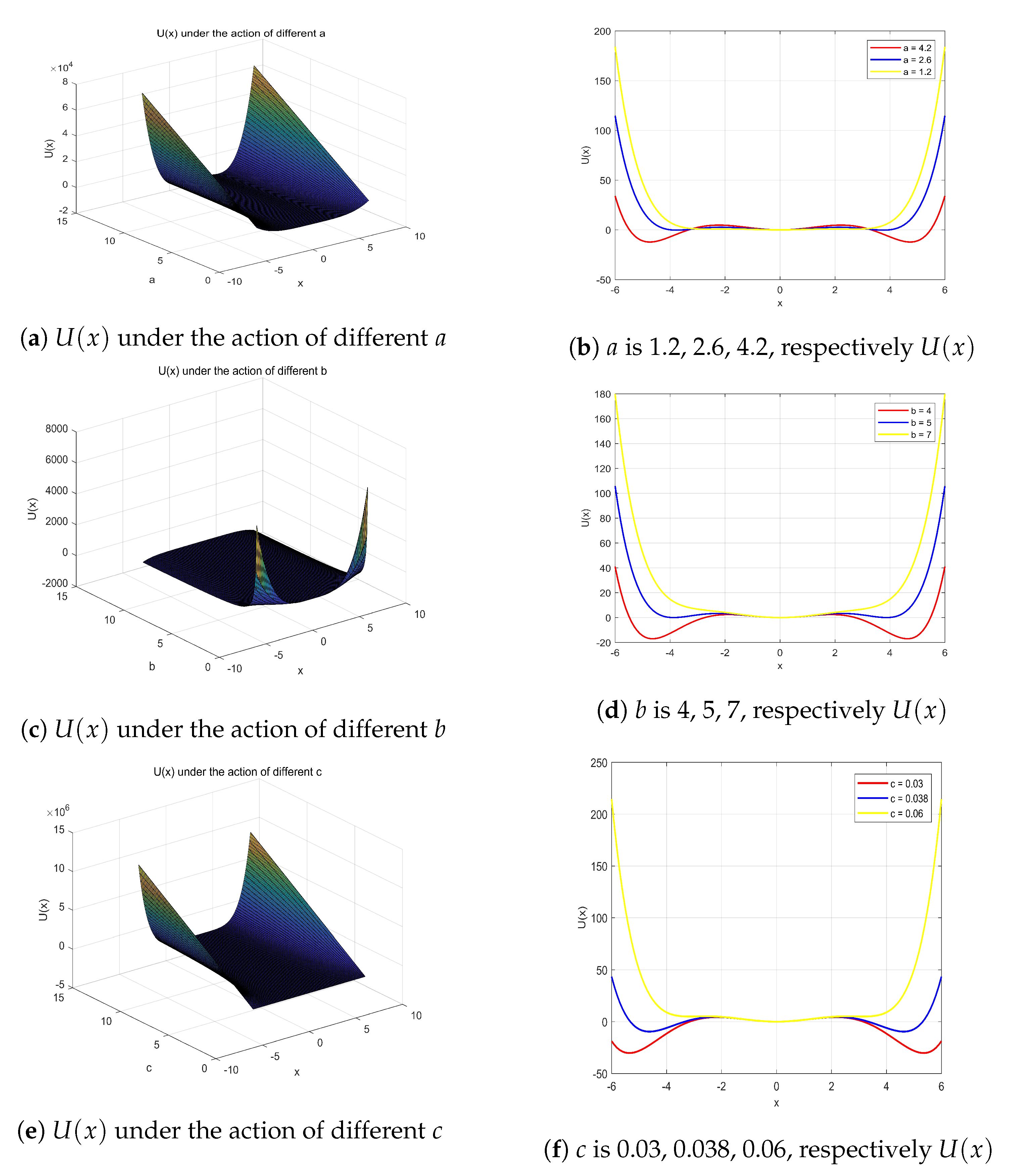
If the multi-stable SR system parameter $b=4.8,c=0.04$ is given, the curve of its potential function and parameter a is plotted, as shown in Figure 3a. Take a for 1.2, 2.6, and 4.2, respectively, and plot the potential function curve, as shown in Figure 3b. It can be seen from the two figures that as the a increases, the depths of the three wells increase, the width of the well becomes wider, and the system is multi-stable; as a continues to increase, the two sides of the well depth will be much larger than the intermediate well depth until the intermediate well depth is reduced to zero, at which point the system switches to bi-stable.

If the multi-stable SR system parameters are $a=3,c=0.04$, the curve of the potential function and the parameter b is plotted as shown in Figure 3c. It can be seen from the figure that as b increases continuously large, the system state gradually switches from multi-stable to mono-stable. Take b as 4, 5, and 7, respectively, and obtain the potential function curve, as shown in Figure 3d. It can be seen from the figure that when b is small, the depth of the intermediate well is smaller than the depth of the left and right wells, and the system is multi-stable; but as b increases, the depth of the intermediate well remains unchanged, and the depth of the wells gradually decreases. Finally, when the depth of the two wells is zero, the system will switch to mono-stable.

It can be seen from Equations (27) and (28) that by changing the system parameters $a,b,c$, the three well depths of the multi-stable potential function can be changed, thereby changing the barrier height and further affecting whether the energy of the particles can be overcome by doing a periodic motion between potential wells. Since the multi-stable system has better detection capability than the mono-stable system and the bi-stable system, the system is selected in a multi-steady state as the system parameters are selected. In order to make the system in a multi-steady state, it is necessary to study the influence of system parameters $a,b,c$ on the system to determine the range of values of each parameter.

First, define the ratio of $\Delta U_M$ and $\Delta U_{L,R}$ to R. Its expression is Equation (38)

$$R=\frac{\Delta U_M}{\Delta U_{L,R}},$$

(38)

It can be seen from the above equation that when $\Delta U_M=\Delta U_{L,R}$, the ratio R is 1, and the energy required for the periodic transition of the particles between each potential well is the same. When $R>1$, which is $\Delta U_M>\Delta U_{L,R}$, the energy required for the particles to transition from the two potential wells to the intermediate well is less than the energy required for the particles to transition from the intermediate well to the two wells. When $R<1$, which is $\Delta U_M<\Delta U_{L,R}$, the energy required for the particles to transition from the intermediate potential well to the two potential wells is less than the energy required for the particles to transition from the two potential wells to the intermediate potential well.

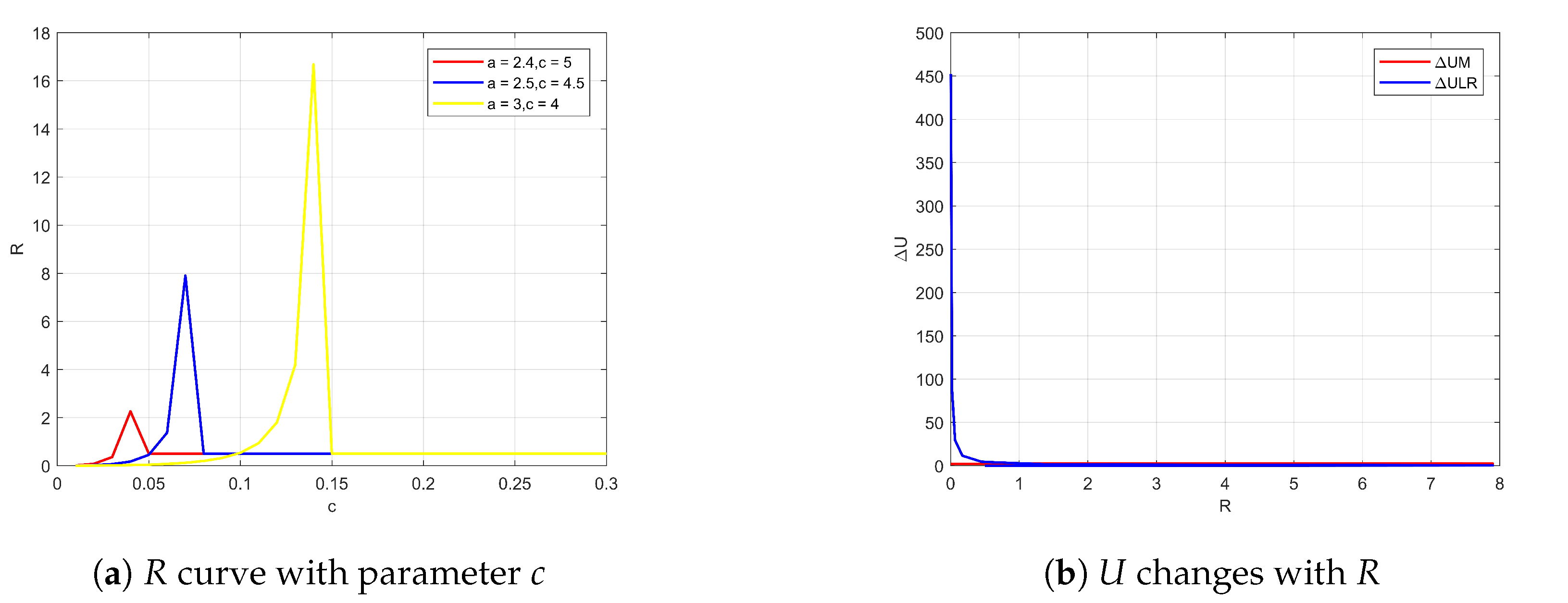
Assume that the input signal amplitude $A_i$ and noise intensity D of the system are both 0, and the variation law of R with the system parameter a is shown in Figure 4.

It can be seen from Figure 5 that when b and c take different values, as a increases continuously, the R value increases first and then decreases, and each R value corresponds to two different a values, When $a=1$, its peak value is reached, that is, the ratio of $U_M$ and $U_{RL}$ is the largest, $R=19.51$. When $a<1$ and $a>1$, $b=5,c=0.038$, the curves of the well depth with R are shown in Figure 5.

It can be concluded from Figure 5 that when $a<1$, as the R increases, the depth of the wells decreases and the depth of the intermediate well increases. When $a>1$, as R increases, three The depth of each well is decreasing continuously. When $R<1$, the depth of the wells on both sides is greater than the depth of the intermediate well, and the energy required for the particles to transition from the intermediate well to the two wells is less than the energy required to transition from the two wells to the intermediate well. When $R=1$, the three wells have the same depth. When $R>1$, the depth of the intermediate well is greater than the depth of the wells on both sides, and the energy required for the particles to transition from the intermediate well to the two wells is more than the energy required for the two wells to transition to the depth of the intermediate well.

At the same time, as shown in Figure 5b, when $R=0.05$, the depth of the wells on both sides is 201.02, and the depth of the intermediate well is about 10.15. At this time, the depth of the wells on both sides is much larger than the depth of the intermediate wells, so the system is approximated to bi-stability; when R = 1, the three wells have the same depth and the system is multi-stable; as R increases, when $R=19.51$, the depth of the wells on both sides is 0.0419, and the depth of the intermediate well is 0.8055. At this time, the depth of the intermediate well is much larger than the depth of the wells on both sides, and the system is approximately mono-stable. Therefore, when the system is multi-stable, that is, when R = [0.05, 20], the value of a ranges from 0.05 to 10.

The SR system parameters when $a=2,c=0.04$, the variation curve of R with the system parameter b, and the variation of the well depth with R are shown in Figure 6.

It can be seen from Figure 6a that when a and c are combined with different values, as R increases, each R increases first and then decreases rapidly to a constant value; when $b>6$, R does not change with the change of b. At this time, its value is constant at 0.5, and the system remains multi-stable. Therefore, when $b<6$, the curve of the well depth with R is plotted, as shown in Figure 6b. When $R=0.05$, the depth of the wells on both sides is about 9.12, and the depth of the intermediate well is about 0.4185. At this time, the depth of the wells on both sides is much larger than the depth of the intermediate well, and the system is approximately bi-stable; at this time, the energy required for the particles to transition from the two wells to the intermediate well is much larger than the energy required for the intermediate well to transition to the two wells. With the increase of R, when $R=20$, the depth of the well on both sides is 0.0502, and the depth of the intermediate well is 0.8458. At this time, the depth of the wells on both sides is much smaller than the depth of the intermediate well, and the system state is approximately mono-stable. Therefore, the system is multi-stable, that is, when $R=[0.05,20]$, the range of b is [1, 10]. If a given system parameter $a=2.4,b=5$, the curve of R with system parameter c and the curve of the potential well with R are shown in Figure 7.

It can be concluded from Figure 7 that R increases first and then decreases rapidly to a constant value as c increases. When $c>0.04$, the R value is stable at a constant value of 0.5, and the system remains multi-stable. It can be seen from Figure 7b that when $R=0.05$, the depth of the wells on both sides is much larger than the depth of the intermediate well, and the system is approximately bi-stable; the energy required for the particles to transition from the two wells to the intermediate well at this time is much larger than the energy required for the intermediate well to transition to the two wells. When $R=1$, the three wells have the same depth and the system is multi-stable; as R increases, the depth of the wells on both sides is almost zero when $R=20$, and the system is approximately mono-stable. Therefore, the system is multi-stable, that is, when $R=[0.05,20]$, the value of c ranges from 0 to 0.3.

According to the above analysis, when $R>20$, the depth of the intermediate well is much larger than the depth of the wells on both sides, and the mono-stable condition occurs easily; when $R<0.05$, the depth of the intermediate well is much smaller than the depth of the wells on both sides, and the system is approximate to bi-stable. Therefore, in order to ensure that the system is multi-stable, the range of R is [0.05, 20], that is, the range of the system parameter a is [0.05, 10], and the range of b is [1, 10], c the value range is (0, 0.3), which lays a foundation for parameter synchronization optimization of adaptive multi-stable SR system.

4. Practical Engineering Application

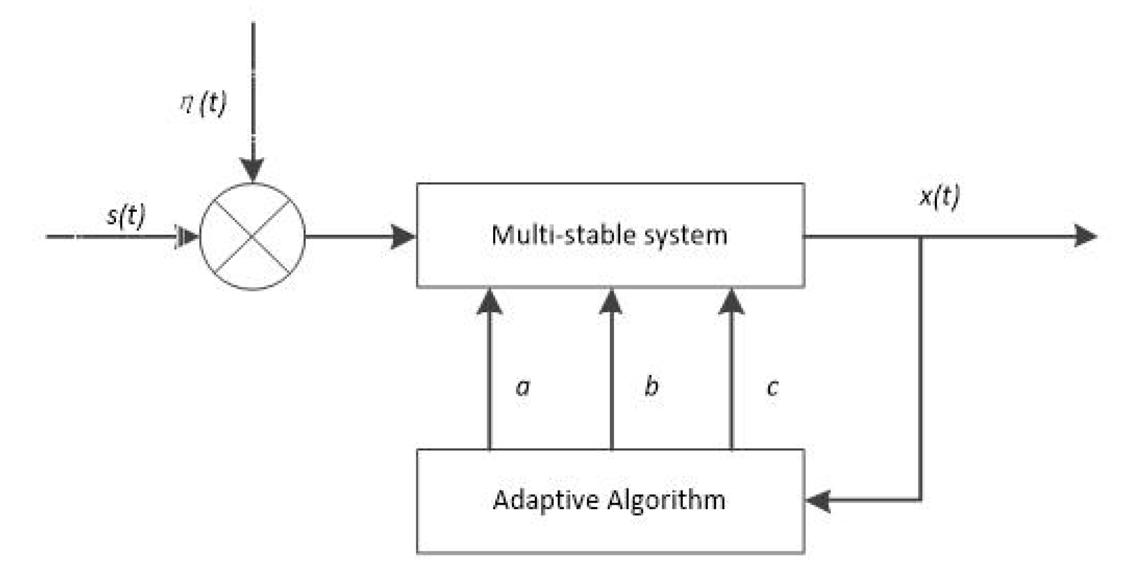
The schematic diagram of the adaptive multi-stationary stochastic resonance structure is shown in Figure 8. The $a,b,c$ parameters of the multi-stable system are updated by analyzing the output signal of the system. The specific workflow is shown in Figure 9. Firstly, the population of the ant colony algorithm is initialized, and then the initial input is input into the multi-stationary stochastic system. The ant colony algorithm is used to determine whether the SNR signal-to-noise ratio is out of range. The pheromone is evaluated to obtain the optimal $a,b,c$ values, even for the optimal solution of the system.

The test platform is shown in Figure 10a as the “Sailfish” AUV. Through the analysis of the AUV dynamics model, it can be seen that the AUV actuator collision, winding, and other faults directly affect the current parameters, so this paper uses the current data after the AUV collision. A collision failure occurs in the AUV experiment, and the spindle bending phenomenon occurs, as shown in Figure 10b.

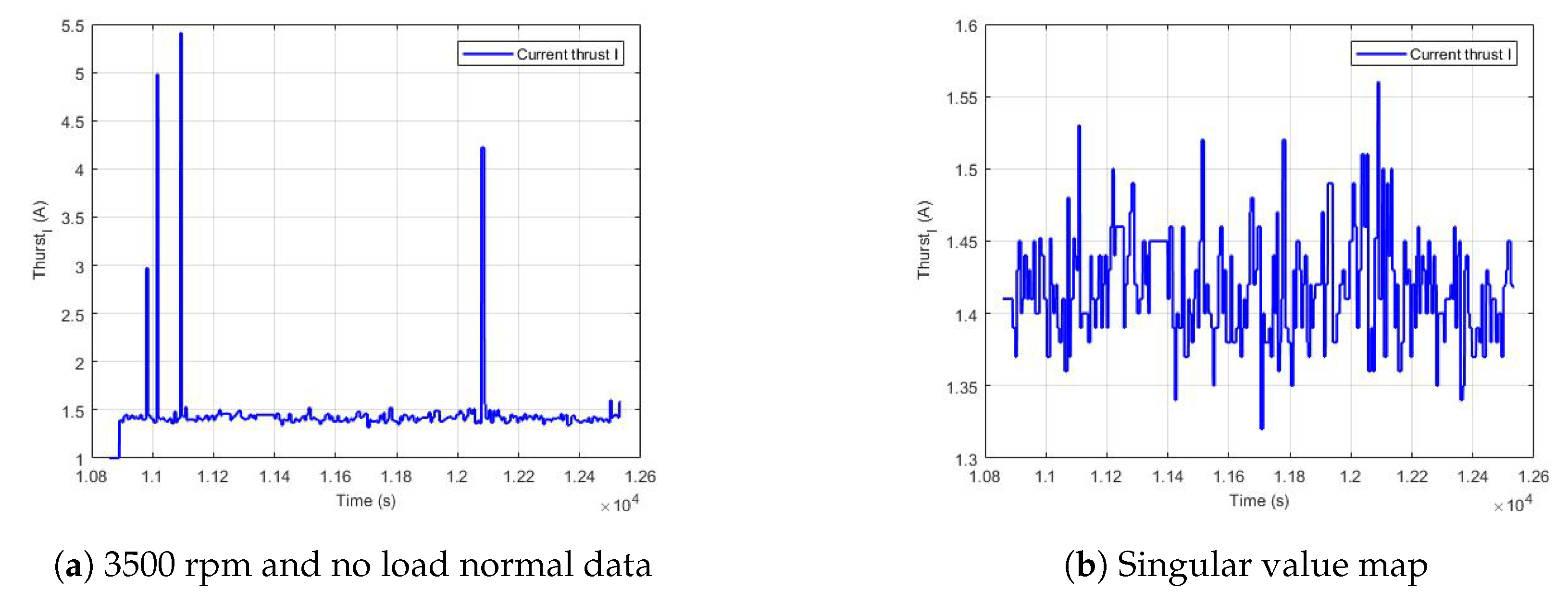
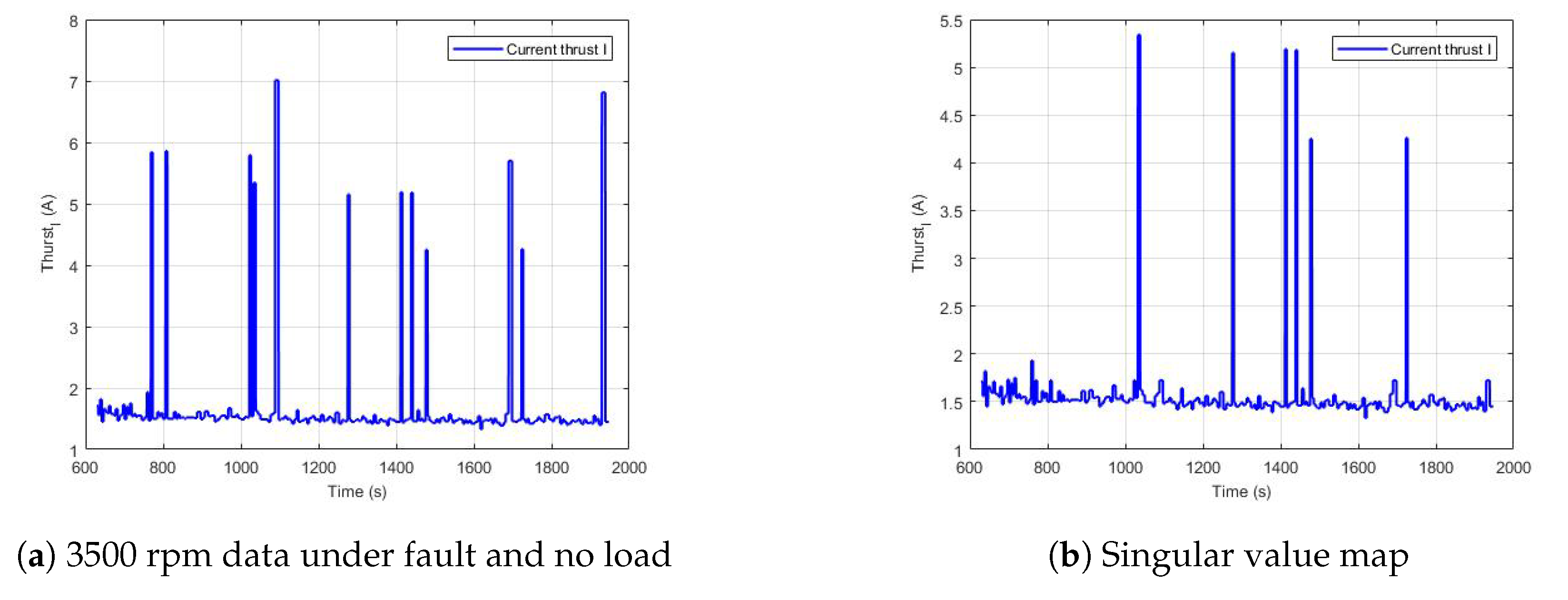
From the experimental data, we can see that the data has unreasonable singular values. It is more appropriate to eliminate the singular value by using the standard deviation method and take four standard deviations. The data for 3500 rpm under normal no load (a) and singular value map (b), and 3500 rpm data under fault no load (c) and singular value map (d) are shown in Figure 11 and Figure 12.

From the experimental data, it can be seen that the current increases obviously, and the number of singular values increases obviously after collision, but it is difficult to judge whether the current increases slightly due to fault under normal navigation conditions. The experimental data are used to verify the bi-stable and tri-stable stochastic resonance fault diagnosis. The noise intensity is 0.05, and the noise function is $A\ast cos(2\ast pi\ast f0\ast tt)$, where $A=0.01$ and $f0=0.008$. The fourth-order Runge–Kutta algorithm is used to solve Equation (26).

$$\left\{\begin{array}{c}x(n+1)=x\left(n\right)+\frac{1}{6}(k_1+2k_2+2k_3+k_4)+h^{\frac{\alpha }{l}}\xi \left(n\right)\hfill \\ k_1=h\left(-ax\left(n\right)+\frac{1+a}{b}{x}^3\left(n\right)-c{x}^5\left(n\right)+s\left(n\right)\right)\hfill \\ k_2=h\left(-a(x\left(n\right)+\frac{k_1}{2})+\frac{1+a}{b}{(x\left(n\right)+\frac{k_1}{2})}^3-c{(x\left(n\right)+\frac{k_1}{2})}^5+s\left(n\right)\right)\hfill \\ k_3=h\left(-a(x\left(n\right)+\frac{k_2}{2})+\frac{1+a}{b}{(x\left(n\right)+\frac{k_2}{2})}^3-c{(x\left(n\right)+\frac{k_2}{2})}^5+s\left(n\right)\right)\hfill \\ k_4=h\left(-a(x\left(n\right)+k_3)+\frac{1+a}{b}{(x\left(n\right)+k_3)}^3-c{(x\left(n\right)+k_3)}^5+s\left(n\right)\right)\hfill \end{array}\right.$$

(39)

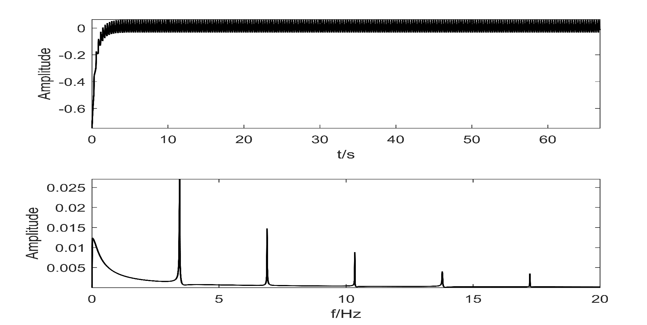
Comparing the spectrum of normal data with fault data, as shown in Figure 13, it is found that the difference between the two is small, so it is difficult to determine whether it is faulty. The fault diagnosis using tri-stable and bi-stable is shown in Figure 14 and Figure 15. The corresponding values are obtained from the adaptive algorithm of ant colony, $a=3.01,b=1,c=0.042,SNR=22.5587$. It can be seen that the tri-stable stochastic resonance has the best diagnostic effect and the highest peak. The normal data is verified under the same parameters. The peak value of the tri-stable system is small, so it can be explained that the system is sensitive to fault signals and insensitive to normal data.

We can see that the bi-stable stochastic resonance part of the signal is submerged in the noise, and the weak fault of collision is not well diagnosed, but the tri-stable system can detect the fault better. Therefore, the effect of the tri-stable system in the collision fault diagnosis of the AUV propeller is better than that of the bi-stable system.

5. Conclusions

The dynamic model of the AUV thruster is analyzed, and the actuator current can be used in the fault diagnosis of the AUV actuator. The tri-stable system is analyzed, and the value range of R is [0.05, 20]. The value range of a is [0.05, 10], the value range of b is [1, 10], and the value range of c is [0, 0.3], which lays a foundation for parameter synchronization optimization of an adaptive multi-stable SR system. The peak value of adaptive bi-stable SR is 0.6, and there is no second peak value. However, the peak value of the normal data is 0.025, which proves that the method can produce stochastic resonance and can be used in fault diagnosis. The ant colony-optimized tri-stable stochastic resonance system can be applied to the weak fault diagnosis of AUV thrusters, and the first peak is 1.8 more than the bi-stable.