Assessing Water Infiltration and Soil Water Repellency in Brazilian Atlantic Forest Soils

Abstract

This study presents the results of the soil hydraulic characterization performed under three land covers, namely pasture, 9-year-old restored forest, and remnant forest, in the Brazilian Atlantic Forest. Two types of infiltration tests were performed, namely tension (Mini-Disk Infiltrometer, MDI) and ponding (Beerkan) tests. MDI and Beerkan tests provided complementary information, highlighting a clear increase of the hydraulic conductivity, especially at the remnant forest plots, when moving from near-saturated to saturated conditions. In addition, measuring the unsaturated soil hydraulic conductivity with different water pressure heads allowed the estimation of the macroscopic capillary length in the field. This approach, in conjunction with Beerkan measurements, allowed the design better estimates of the saturated soil hydraulic conductivity under challenging field conditions, such as soil water repellency (SWR). This research also reports, for the first time, evidence of SWR in the Atlantic Forest, which affected the early stage of the infiltration process with more frequency in the remnant forest.

1. Introduction

The United Nations has declared the period 2021–2030 the decade of restoration to scale up existing initiatives, such as the Bonn Challenge, to restore degraded ecosystems [1]. It is expected that restoration will not only help to slow climate change through carbon sequestration, provide food, and increase biodiversity [2], but will also have hydrological benefits because of the perceived association between forest cover and soil hydrological ecosystem services [3,4]. In this context, it is necessary to better understand the consequences of forest regrowth on soil hydrological processes, such as water infiltration, which is fundamental to maintain productive soil-water-plant interactions, and also to control soil erosion and runoff, soil moisture content, and groundwater recharge in the ecosystems [5,6,7].

Estimating saturated and unsaturated soil hydraulic conductivities is crucial for interpreting and modeling soil hydrological processes. In addition, knowledge of these properties may provide information on the impact of land use on soils characteristics [8], which are rarely considered in studies of forest restoration [9]. During the last years, many infiltration methods and devices have been developed to determine soil hydraulic properties [10]. Among them, the Beerkan method [11] is becoming very popular in soil science because it constitutes a simple and an inexpensive way to determine the saturated soil hydraulic conductivity, K_s, in the field [12,13]. On the other hand, the mini-disk infiltrometer (MDI) is a routinely used method for measuring infiltration rates under negative pressure head in the field. The MDI is easily transportable and easy to use on hillslopes, thus, it substantially facilitates the replicability of the measurements [10].

Our previous study in the Atlantic Forest of Brazil [14] used the Beerkan protocol at three land covers, namely pasture, 9-year-old restored forest, and remnant forest. Our results showed that water repellency impacted water infiltration, yielding convex shaped cumulative infiltration curves. However, this observation was not carefully assessed. Similarly, many studies on tropical soils have reported some indirect effects of water repellency on water infiltration, such phenomenon is still poorly documented, especially in comparison with temperate regions [5,15,16,17]. Soil water repellency (SWR) or hydrophobicity is a transient soil property with which soils increase the resistance to wetting and infiltration. It is spatially and temporally very variable [18,19]. This is caused mainly by amphiphilic molecules produced by plants and organism, and generally occurs after forest fires or dry periods. Other factors that can be related to water repellency are the soil texture, soil temperature, pH, water content, soil organic carbon, land use, and plant cover [18,19,20,21]. In addition, recent research highlighted that climate change could increase the water repellency of soils, due to the increasing occurrence of extreme events such as droughts, which create the soil conditions (i.e., high temperatures and low soil water content) that promote the water repellency [22].

Currently SWR is receiving increased attention in the scientific literature, due to the important hydrological effects. For example, SWR reduces infiltration capacity, increases runoff rates as well as leaching of agrochemicals and soil erosion, also it can affect negatively the crop production, nutrients, and plant-available water [17,23,24]. On the other hand, SWR has positive impacts on soil aggregate stability and organic carbon sequestration [22]. Müller and Deurer [17] reported the benefit of SWR for the arid and semi-arid climates, considering that this soil property reduces the loss of soil water by evaporation and allows the rainwater to reach deeper depths. Despite these efforts, our understanding of SWR is still limited [18], especially when subcritical phenomena occur.

This investigation aims to broaden our previous work [14], using the same location in the Brazilian Atlantic Forest. In particular, the specific objective was to compare both unsaturated and saturated soil hydraulic conductivity determined with simple and low-cost field infiltration methods (MDI and Beerkan), for three land covers, namely pasture, 9-year-old restored forest, and remnant forest. This paper includes the first measurements of SWR in the Brazilian Atlantic Forest and its relevance regarding soil hydraulic properties, which had never been investigated so far, to the best of our knowledge.

2. Materials and Methods

2.1. Field Sites and Soil Sampling

The study area (22˚53′ S, 46˚54′ W) is located in the county of Campinas, São Paulo State, Southeast Brazil. The area is located inside the sub-basin of Atibaia River (2800 km²), which belongs to the Piracicaba River basin. The vegetation is classified as seasonal semideciduous forest. The zone is characterized by a complex geology located at the transition between the Atlantic Plateau and the Peripheral Depression geomorphological provinces, with Ultisols and Entisols as main soils [25]. The elevation varies from 600–900 m a.s.l. The climate is classified as Cwa according to the Köppen classification, with annual rainfalls of 1700 mm and mean annual temperature of 20 °C [26].

The three investigated land covers (pasture, P, restored forest, R, and remnant forest, F) correspond with those of Lozano-Baez et al. [14], with the use of the same 18 plots (7 × 7 m in size). These plots represent two pasture (P1 and P2), two restored forest (R3 and R4), and two remnant forest (F5 and F6). Each of these sites is further divided into three blocks (i.e., upslope, U, midslope, M, and downslope, D). For a detailed description of the field sites, the reader may refer to our previous work [13]. In brief, for a given plot, three undisturbed soil cores (5 cm in height and 5 cm in diameter) were collected at the 0–5 cm depth. With these samples we determined in the laboratory the initial volumetric soil water content, θ_i (cm³ cm⁻³), and the soil bulk density, ρ_b (g cm⁻³). Three disturbed soil samples (0–10 cm depth) were also collected to determine the soil texture and the soil organic carbon content (OC). The soil texture was determined by the hydrometer method [27] and the OC was determined by the Walkley-Black method.

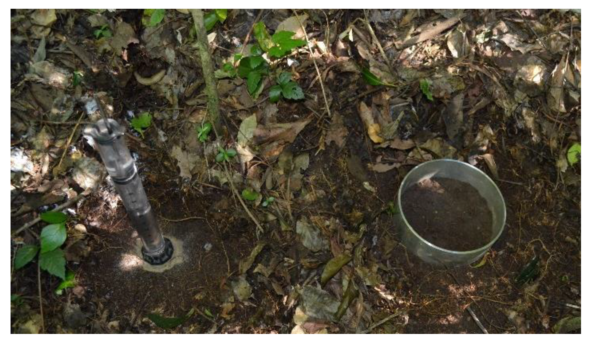
2.2. Unsaturated and Saturated Soil Hydraulic Conductivity Measurements

Unsaturated soil hydraulic conductivity was measured using the Mini-Disc Infiltrometer (MDI) [28]. A total of 108 MDI experiments were carried out in the study sites. At each plot, we randomly selected six points with a minimum distance between measurements of 2 m. At the same sampling point, we used three different water pressure head values, h, in the ascending sequences −20, −5, and 0 mm, in order to sample several subdomains of the pore size distribution. Unsaturated soil hydraulic conductivity was calculated according to the method proposed by Zhang [29]. Before the MDI tests started, we removed the litter and leaves, and the sampled soil surface was gently levelled and smoothed. We used a thin layer of fine sand to ensure the contact between the infiltrometer and the soil (Figure 1). The thickness of the layer of sand was negligible and did not modify the imposed pressure head of the MDI. Visual readings of the water level were taken every 30 s until steady infiltration was nearly reached. For further descriptions of the MDI, details of measurements and calculations of hydraulic conductivity see Decagon Devices Inc. (Washington, DC, USA) [28].

The saturated soil hydraulic conductivity, K_s (mm h⁻¹), was measured with ponding infiltration experiments of the Beerkan type [13]. At each plot, we performed seven Beerkan tests, for a total of 126 experiments. We used a steel ring with an inner diameter of 16 cm inserted to a depth of about 1 cm into the soil surface (Figure 1). In each infiltration point, a known volume of water (150 mL) was repeatedly poured into the cylinder at a small height above soil surface (i.e., a few cm) and the energy of the water was dissipated with the hand fingers to minimize the soil disturbance. Then, the time needed for each poured volume to complete infiltration was logged. This procedure was repeated until the difference in infiltration time between three consecutives trials became negligible.

The equilibration time, t_s (s), namely the duration of the transient phase of the infiltration process, was estimated according to the suggested criterion by Bagarello et al. [30] for analyzing cumulative infiltration data. More specifically, the t_s value was determined as the first value for which:

$$\widehat{E}=\left|\frac{I\left(t\right)-I_{reg}\left(t\right)}{I\left(t\right)}\right|\le E$$

(1)

where I_reg(t) is estimated from regression analysis considering the last points, and E defines a given threshold to check linearity. Equation (1) is applied from the end of the experiment until finding the first data point that fits the condition $\widehat{E}$ ≤ E [31,32]. An illustrative example of t_s estimation using the commonly used value of E = 2% [30] is shown in Figure 2a. Transient infiltration conditions therefore occur from time 0 until time t_s (i.e., when $\widehat{E}$ > 2), while steady-state conditions establishes for all data points measured after time t_s (i.e., when $\widehat{E}$ ≤ 2).

At the end of each infiltration test, we collected a disturbed soil sample within the infiltration surface to determine the saturated gravimetric water content, and thus the saturated volumetric water content, θ_s (cm³ cm⁻³), considering the values of dry bulk density, ρ_b, previously determined.

2.3. Estimating the Saturated Soil Hydraulic Conductivity, K_s

We estimated K_s by the Simplified method based on the near Steady-state phase of a Beerkan Infiltration run (SSBI), recently proposed by Bagarello et al. [32]. This method estimates K_s through an infiltration experiment of the Beerkan type [13] and an estimate of the macroscopic capillary length, λ_c (mm), expressing the relative importance of the capillary over gravity forces during water movement in unsaturated soil [33,34,35]. Firstly, the experimental steady-state infiltration rate, i_s (mm h⁻¹), is estimated by linear regression analysis of the last data points of the cumulative infiltration, I (mm), versus time, t (h), plot, describing the near steady-state condition. Then, SSBI estimates the saturated soil hydraulic conductivity, K_sS (mm h⁻¹) (the subscript S is used to indicate SSBI), as follows [33]:

$$K_{sS}=\frac{i_s}{\frac{{\mathsf{\gamma }\mathsf{\gamma }}_w{\mathsf{\lambda }}_c}{r_d}+1}$$

(2)

where γ and γ_w are dimensionless constants [36,37] related to the infiltration front shape, that are commonly set at 0.75 and 1.818, and r_d (mm) is the radius of the containment ring. Two different scenarios were considered to apply the SSBI method. The first scenario considered the MDI experiments, carried out with pressure heads of $h_{-20}$ = −20 mm and $h_0$ = 0, to estimate λ_c by the following equation [38]:

$${\lambda }_c=\frac{h_{-20}-h_0}{ln\left(Q_{s,h_{-20}}/Q_{s,h_0}\right)}$$

(3)

where $Q_{s,h_{-20}}$ and $Q_{s,h_0}$ (mm³ h⁻¹) are the steady flow rates corresponding to $h_{-20}$ and $h_0$, respectively, and they were estimated as follows:

$$Q_s={\mathrm{i}}_{\mathrm{s}}{\mathsf{\pi }\mathrm{r}}_{\mathrm{d}}{}^2$$

(4)

For this scenario, we firstly averaged for each plot the individual i_s values, then plot-dependent λ_c values were estimated by Equation (3) (Table S1).

The second K_sS dataset was obtained considering λ_c = 83 mm, since it represents the suggested first approximation value for most soils types [37,39].

The Beerkan Estimation of Soil Transfer parameters (BEST) method [11] was also applied to estimate the saturated soil hydraulic conductivity, K_sB (mm h⁻¹) (the subscript B is used to indicate BEST). More specifically, among the three existing BEST algorithms, we used the BEST-steady algorithm [40], that estimates K_sB, by the following equation [41]:

$$K_{sB}=\frac{{\mathrm{C} \mathrm{i}}_{\mathrm{s}}}{{\mathrm{A} \mathrm{b}}_{\mathrm{s}}+\mathrm{C}}$$

(5)

where b_s (mm) is the intercept of the regression line fitted to the last data points of the I versus t plot. The A (mm⁻¹) and C constants are defined for the specific case of the Brooks and Corey [42] relation and taking into account soil moisture initial conditions as follows [36]:

$$A=\frac{\mathsf{\gamma }}{{\mathrm{r}}_{\mathrm{d}}\left({\mathsf{\theta }}_{\mathrm{s}}-{\mathsf{\theta }}_{\mathrm{i}}\right)}$$

(6)

$$C=\frac{1}{2\left[1-{\left(\frac{{\mathsf{\theta }}_{\mathrm{i}}}{{\mathsf{\theta }}_{\mathrm{s}}}\right)}^{\mathsf{\eta }}\right]\left(1-\mathsf{\beta }\right)}\ln \left(\frac{1}{\mathsf{\beta }}\right)$$

(7)

where β is a coefficient commonly set at 0.6, and η is a shape parameter that is estimated from the analysis of the particle size data with the pedotransfer function included in the BEST procedure [11].

Following Bagarello et al. [32], the BEST-steady algorithm was chosen to check the SSBI method, compering K_sS and K_sB in terms of factors of difference, FoD, calculated as the highest value between K_sB and K_sS divided by the lowest value between K_sB and K_sS. Differences between K_sS and K_sB not exceeding a factor of two were considered indicative of satisfactory K_s predictions [33].

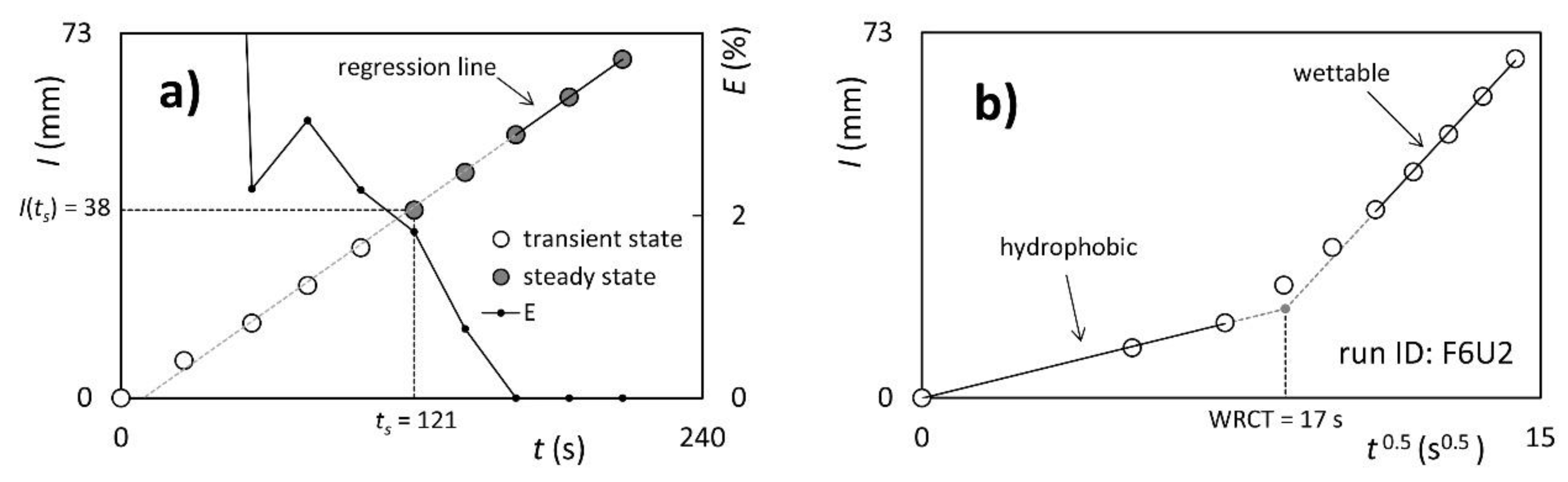
2.4. Soil Water Repellency Carachterization

Some of the Beerkan runs provided cumulative infiltration curves with convex shapes, signaling the occurrence of SWR phenomena [43,44].Then, the water repellency secession time, WRCT (s), was estimated from the intersection point of two straight lines, representing the initial and the late stages of I vs. t^0.5 relationship [45,46] (Figure 2b). The persistence of water repellency was measured using the water drop penetration time (WDPT) test. This test is widely used to determine the persistence of water repellency, it is easy to perform in field and presents the hydrological implications of hydrophobicity, because the amount of surface runoff is affected by the time required for the infiltration of droplets [47]. At each plot, we selected five sampling points. The WDPT was carry out by placing 10 drops (0.05 mL) of distilled water on to the soil surface and recording the time for their complete infiltration. Following other investigations [48,49] the infiltration recording was stopped after 3600 s. Moreover, if the drop did not infiltrate after this time interval, the value of 3600 s was assigned for the WDPT [47].

2.5. Data Analysis

Following similar investigations [10,12,14], unique values of clay, silt, sand, OC, ρ_b, θ_i, and θ_s were determined for each plot by averaging the measured values. For these soil parameters, we assumed a normal distribution, thus no transformation was performed on these data before statistical analysis. In addition, the K_sB, K_sS, K_–20, K_–5, K₀, and WDPT data were assumed to be log-normally distributed since the statistical distribution of these data is generally log-normal [50]. Statistical comparison was conducted using two-tailed t-tests, whereas the Tukey Honestly Significant Difference test was applied to compare our data set. The ln-transformed K_sS, K_sB, K_–20, K_–5, K₀ and WDPT data were used for the statistical treatment. A probability level, α = 0.05, was used for all statistical analyses. It is reasonable to presume that infiltrometer data can also vary depending on the initial soil moisture and its effect on SWR [31], therefore the Spearman’s rank correlation coefficients (r) were used to evaluate the relative influence of the soil properties on the infiltration process. For all the statistical analyses the Minitab© computer program (Minitab Inc., State College, PA, USA) was used.

3. Results and Discussion

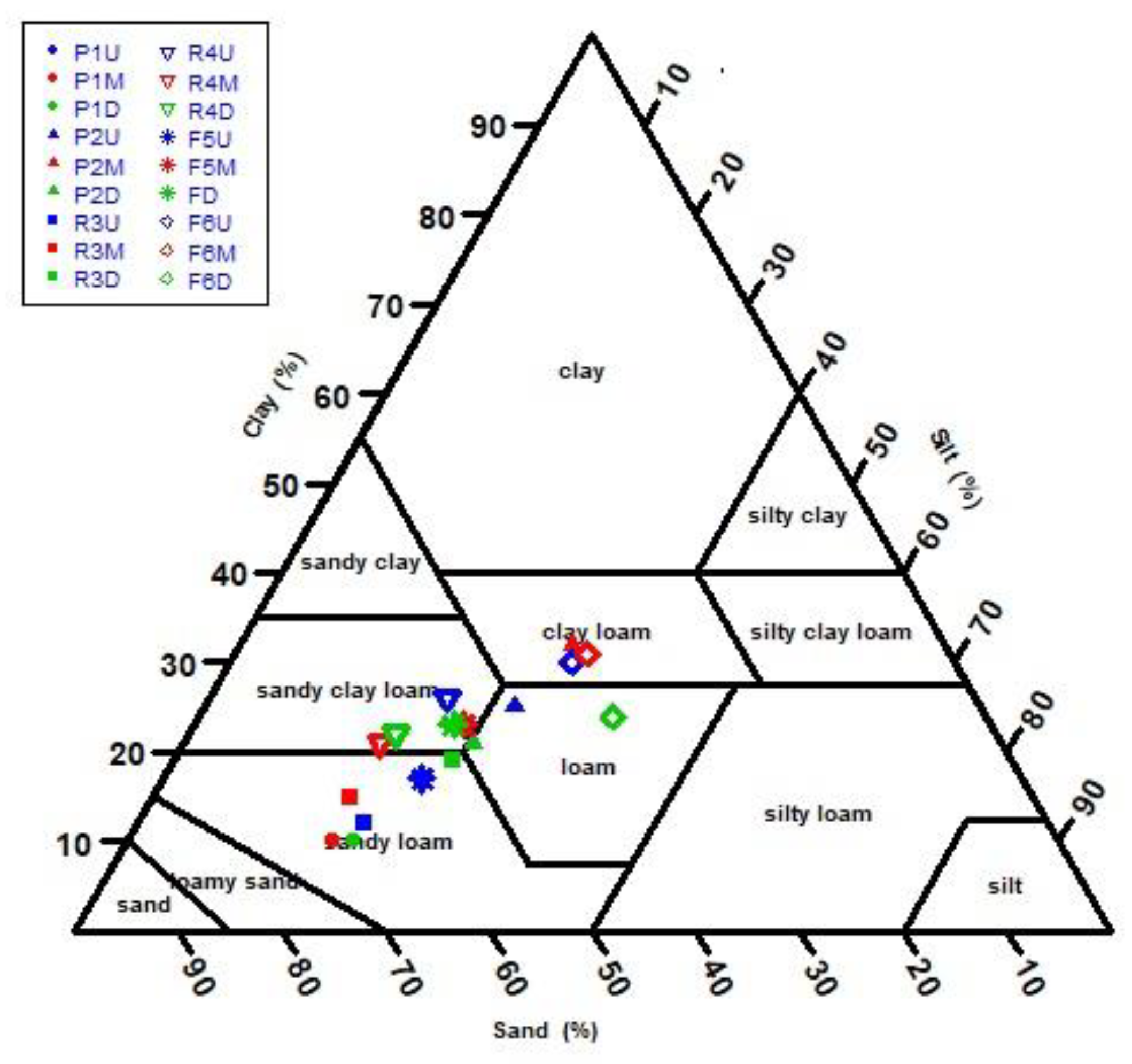
3.1. Soil Properties

The 18 plots showed appreciable differences in soil texture. Sandy loam (i.e., P1M, P1D, R3U, R3M, R3D, and F5U) and sandy clay loam (i.e., P1U, R4S, R4M, R4D, F5M, and F5D) were the dominant soil textures among the plots, followed by clay loam (i.e., P2M, F6U, and F6M) and loam (i.e., P2U, P2D, and F6D). The soil texture of the plots is presented in the USDA textural triangle (Figure 3).

As pointed out by our previous study [14], the OC at the pasture sites in the soil depth 0–0.10 m was similar to remnant forest, while restored forest sites presented the lowest OC values. The highest ρ_b values were observed in the restored forest R4, where the exposure of the soil and trampling pressure during the land-use history was greater in comparison with restored forest R3. Forest soils were characterized by the lowest ρ_b values, which can be related to the heterogeneous soil structure and higher soil macroporosity in this cover [51,52]. At the time of sampling, the θ_i ranged from 0.12 to 0.32 cm³ cm⁻³ and the soil was significantly wetter in plots P1U, P2M, R4S, R4M, and F5I (Figure S1).

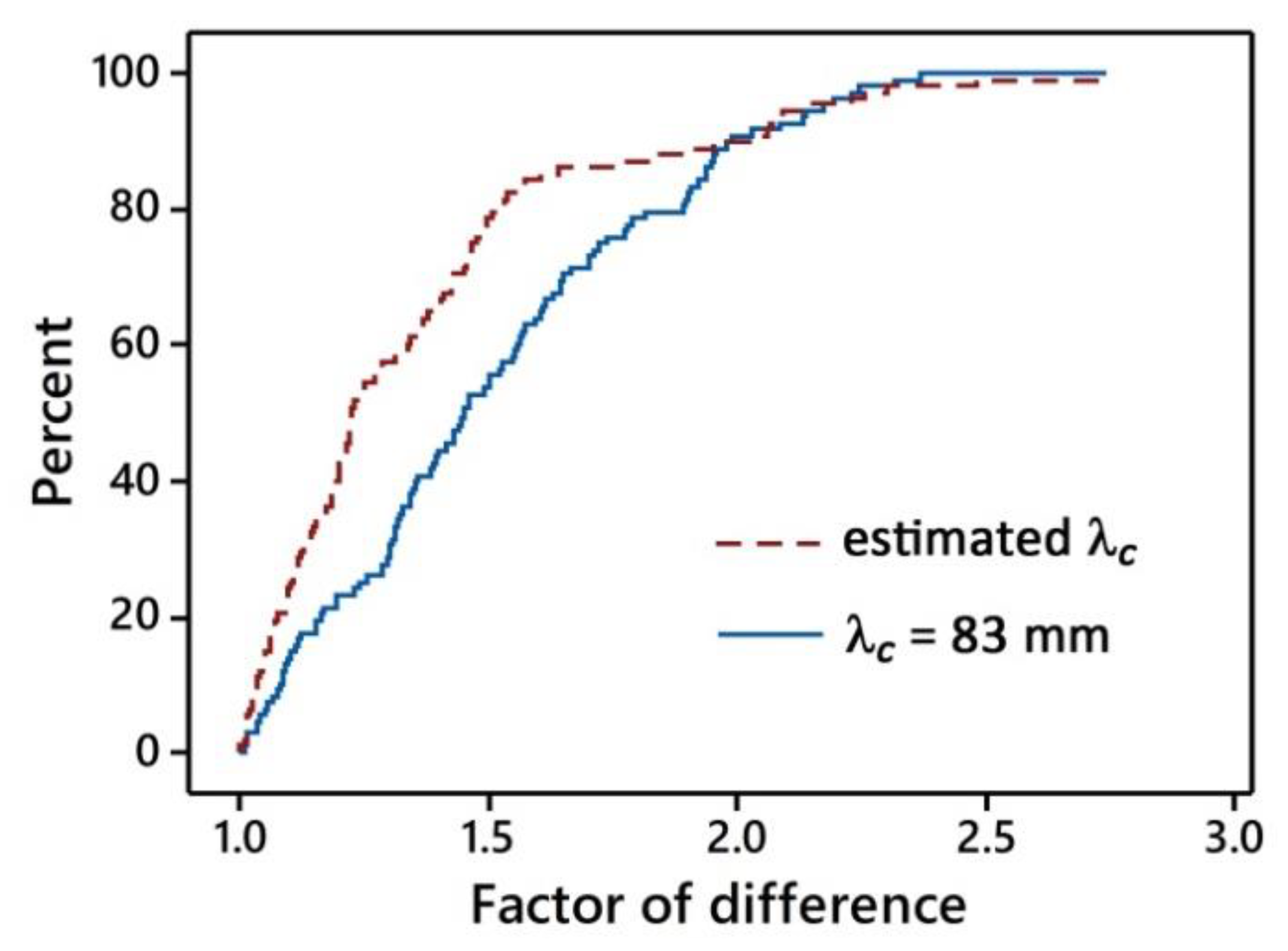
3.2. Assessing SSBI Estimates

Both SSBI scenarios always yielded physically plausible estimates (i.e., positive K_s values). For the first scenario (i.e., λ_c estimated from multi tension experiments), the K_sS values ranged between 5.9 and 1486.8 mm h⁻¹. The mean FoD was equal to 1.36 (maximum value = 2.74) and the individual values were less than 2 and 1.5 for 89% and 78% of the cases, respectively (Figure 4). For the second scenario (i.e., λ_c = 83 mm), K_sS data ranged between 3.7 and 934.5 mm h⁻¹. The mean FoD was equal to 1.51 (maximum value = 2.37) and the individual values were less than 2 and 1.5 in the 90% and 53% of the cases, respectively. Therefore, using the estimated λ_c values resulted in a slightly better estimation of K_sS, yielding a lower mean FoD value, thus, only the first scenario was considered in the subsequent analysis.

3.3. Comparing BEST versus SSBI Estimates Under Soil Water Repellency Conditions

BEST-steady failed to estimate K_s in case of convex-shaped cumulative infiltration curves, which led to negative b_s values and consequently to null K_sB. The K_sB data ranged between 4.5 and 1394 mm h⁻¹ (almost three orders of magnitude). The BEST-steady algorithm yielded physically plausible estimates (i.e., positive K_s values) for 108 of 126 infiltration runs (i.e., 85.7% of cases). The percentage of successful runs was of 95.2% both for the pasture and restored forest (40 of 42 runs). With reference to the remnant forest, BEST led to a failure rate value of 33.3%, leading to lacks of estimates for 14 of 42 infiltration runs. In these cases, cumulative infiltration curves had convex shapes, which are typical for hydrophobia i.e., [42,45,46]. Such hydrophobia may result from significant amounts of organic matter content i.e., [52,53,54], originating from fauna and flora activities [55]. Soil texture also plays a major role on SWR, in particular, SWR is expected to increase for decreasing clay content. In this sense, our plots (i.e., F5U, R3U, R3D, P1M) with more sand content exhibited higher WDPT values. On the other hand, for the forest plots (i.e., F6U, F6M, F6D) the significant amounts of organic matter had a main role in generating relevant WDPT values also on finer textured soils [23,56].

The BEST-steady algorithm was unable to provide positive K_s values, showing that BEST can only be used when the soil does not exhibit hydrophobic effect, as suggested by Lassabatere et al. [57]. As shown in Figure 5, at increasing failure rates of the BEST method corresponded higher WDPT values, suggesting that where hydrophobic condition occurred, mainly in the remnant forest plots, it was the main cause of failure of BEST-steady. More specifically, BEST-steady requires both the slope and the intercept of regression line fitted to the last data points on the I vs. t plot. The magnitude of b_s depends on the entire cumulative infiltration curve (including the transient phase) [58,59], therefore that term is sensitive to SWR that impedes the early wetting phase of the infiltration process. When soil hydrophobicity occurred, the I vs. t^0.5 plot exhibited the characteristic “hockey-stick-like” shape [46], hiding the estimation of K_s trough BEST-steady [42]. On the other hand, SSBI differs by the term expressing steady-state condition, considering exclusively the final infiltration rate [13]. The exclusive use of this term allowed to consider only the final stage of the infiltration process, i.e., when the hydrophobicity effect on infiltration was diminished. In this investigation eighteen Beerkan infiltration tests exhibited a clear hockey-stick-like shape, mainly at the remnant forest plots, that allowed calculation of WRCT as the intersection point of two straight lines, representing the initial and the late stages of I vs. t^0.5 relationships [45] (Figure 2b).

Table 1. Values of the intercept, b_s (mm) of regression line fitted to the last data points describing the steady-state conditions on the I vs. t plot, total duration, t_end (s), total infiltrated depth, I_end (mm), infiltrated depth at the equilibration time, I(t_s) (mm), equilibration time, t_s (s), and water repellency cessation time, WRCT (s), for the eighteen Beerkan infiltration runs affected by hydrophobicity.

ID	bs (mm)	tend (s)	Iend (mm)	I(ts) (mm)	ts (s)	WRCT (s)
P1M6	−13.2	5053	52.7	30.1	3290	93
P1M7	−8.1	4601	45.2	22.5	2678	89
R3U2	−4.7	457	52.7	30.1	277	25
R3D7	−2.1	327	52.7	22.5	145	20
F5U1	−8.4	363	82.9	45.2	210	23
F5U2	−2.7	329	82.9	7.5	39	21
F5U3	−6.4	325	75.3	22.5	115	22
F5U4	−10.4	682	75.3	45.2	439	33
F5M2	−3.3	219	75.3	22.5	72	17
F5M3	−3.3	160	60.2	37.6	103	15
F5M4	−10.7	245	97.9	22.5	74	19
F6U1	−2.3	474	67.8	22.5	166	26
F6U2	−3.2	207	67.8	37.6	121	17
F6U5	−13.3	188	75.3	52.7	140	18
F6M5	−10.4	495	82.9	37.6	253	27
F6M6	−4.3	208	82.9	22.5	64	17
F6D2	−10.1	148	82.9	60.2	112	14
F6D4	−1.3	325	75.3	52.7	229	20

shows the results of the WRCT and the equilibration time calculations. Water repellency always affected the very early stage of the infiltration process since the WRCT values raged between 14 and 93 s, and they were always lower than the t_s values. Therefore, for all the experiments steady-state infiltration rates (i_s) were always reached before the end of the runs and after that the influence of hydrophobicity had ceased, so the K_s values estimated by the use of the SSBI method could be always properly estimated considering the last data points of the infiltration curves. Limiting the hydraulic characterization to the stabilized phase avoided the uncertainties due to specific shape of the cumulative infiltration and a no clear distinction between the early- and late-time infiltration process because soil hydrophobic phenomena [58]. In other words, the results presented in this study suggest that if hydrophobicity affects the first stage of a Beerkan infiltration test, the SSBI estimates should characterize the hydraulic property of the soil properly. We believe that this result has practical importance because the use the SSBI method allowed us to maintain the integrity of the dataset, and to compare the hydraulic behavior of different sites with different land uses, where soil hydrophobicity only occurs in some circumstance.

Moreover, maintaining a small water head on the soil surface may be useful to study the infiltration process in macroporous repellent soils [48]. The SSBI method, covering the soil surface with a practically null depth of water, hence, lower than the commonly water-entry values for repellent soils [59], could allow the operator to characterize water infiltration occurring through either structural or other gaps in the water repellent layer or as fingered flow through zones of hydrophilic or less water repellent soil [60]. On the contrary, establishing several cm of ponded head of water on the infiltration surface is expected to overwhelm SWR [61]. In this investigation, the detection of hockey-stick-like shapes suggested that maintaining a small water head on the soil surface helped to prevent excessive positive pressure from overcoming SWR [62], and allowed the detection of water repellency.

Lower SWR was detected in wetter soils. The correlation between θ_i and ln(WDPT) was significant (r = −0.67, p = 0.002) (

Table 2. Spearman’s rank correlation coefficients of the hydraulic measured properties.

Variables	θi	ln(WDPT)	ln(KsS)
ln(WDPT)	−0.67
p-Value	0.002
ln(KsS)	−0.59	0.74
p-Value	0.009	<0.001
ln(KsB)	−0.61	0.73	0.97
p-Value	0.007	0.001	<0.001

). This result was in line with the reasoning that the soil water content governs the interaction between soil particles and amphiphilic organic molecules, resulting from degradation of tree tissues, that coat soil particles and may be responsible for SWR [45]. The transition from wettable to hydrophobic status (and vice versa) is generally associated to a critical range of soil moisture [63]. The lower water content of this range defines the condition below which the medium is water repellent, the higher identifies the condition above which the medium is wettable. K_s data were positively correlated to ln(WDPT). This is logical, since both macropore flow (which affects the magnitude of K_s) and water repellency phenomena were relevant at the remnant forest plots. In brief, the correlation between these two variables is not the result of a causal connection but the concomitancy of two processes: hydrophobia and macropore flow, which also lead to mainly subcritical water repellency. In addition, we conclude that hydrophobia had no effect on the estimation of the saturated hydraulic conductivity. Indeed, in opposite case, K_sS and ln(WDPT) would have a negative correlation. Consequently, we assumed that the SSBI method proved efficient for detecting SWR and estimating properly the soil saturated hydraulic conductivity, at the same time. Lastly, K_sB and K_sS had a positive correlation with a value close to unity. The two estimators provide close estimates, as discussed above with the FoD. We then can conclude that soil hydrophobicity only affected the failure rate of the BEST-steady algorithm (Figure 5), without affecting the quality of its estimate when the method worked.

3.4. Unsaturated versus Saturated Soil Hydraulic Conductivity

The two types of infiltration tests, i.e., tension and ponding experiments, highlighted a clear increase of the hydraulic conductivity, especially at the remnant forest plots, when moving from near-saturated to saturated conditions (Figure 6). It is important to underscore that saturated and unsaturated conditions could be affected by the different soil texture. Our previous study [14] shows that soils with higher clay content (i.e., P2M, F6M, F6D) evidenced greater variations, by contrast, sandy soils (i.e., P1U, P1M, F5D) had lower variation. The mean values of the ratios between saturated, K_sS, and near-saturated soil hydraulic conductivity, K_–20, were 10.7, 21.5, and 118.3, for the pasture, restored forest and remnant forest, respectively. A similar trend was also detected when the K_–5 values were considered, with the mean values of the ratios equal to 2.2, 5.6, and 23.7. Similar results were also obtained when K_sB values were considered, with the values of the ratios equal to 10.6, 17.5, 92.0, and 2.2, 4.6, 17.4, for the K_–20 and K₅ data, respectively. We also noticed a discrepancy between K_sS and K₀ data, especially at the Forest site, because only under ponded conditions at the surface the macropores are activated [63]. The increase of the difference between saturated and unsaturated conditions can be explained by the activation of macroporosity at the forest plots [64]. Overall, the soil in the remnant forest is heterogeneous and characterized by a dominance of complex macropores. For example, a higher soil macroporosity and total porosity have been reported in the same forest soil by our previous work [14]. This soil macroporosity resulted from the better soil structure, which is caused by the high amount of biopores, roots, soil fauna activity and greater inputs of organic matter [52,63,64]. Moreover, soil variability at the scale of a few meters could have been less represented by the MDI, due to the small diameter of the infiltrometer (i.e., 4.5 cm).

4. Conclusions

To improve the soil hydraulic characterization of the soils under different land uses in the Atlantic Forest of Brazil, we measured and compared the unsaturated and saturated soil hydraulic conductivity, using the MDI and Beerkan method for three land covers, namely pasture, 9-year-old restored forest, and remnant forest. This research reports, for the first time, provide evidence of SWR in the Atlantic Forest, especially in the remnant forest. Our measurements demonstrated that SWR affected the early stage of the infiltration process. The comparison between alternative methods to estimate K_s allowed to account for the effect of SWR on water infiltration measurements. In particular, when there are evidences of SWR, our results suggest using the SSBI method instead of BEST-steady to avoid the failure of the analysis in case of string SWR. Indeed, the SSBI method allowed to maintain the integrity of the infiltration dataset, facilitating the hydraulic comparison between different land uses. Tension (MDI) and ponding (Beerkan) infiltration tests provided a complementary information, highlighting a clear increase of the hydraulic conductivity, especially at the remnant forest plots, when moving from near-saturated to saturated conditions. This information is relevant to assess the infiltration recovery after forest restoration, as it signals soil structure heterogeneity and higher soil macroporosity. In addition, measuring the unsaturated soil hydraulic conductivity with different water pressure heads also allowed to estimate λ_c in the field. This approach, in conjunction with Beerkan measurements, allowed to generate better K_s estimates based on field measurements, and also avoided any subjectivity caused by assuming a constant λ_c value, which is often selected based on general descriptions of soil textural and structural characteristics when estimating K_s from ponding infiltration experiments [34]. Nonetheless, developing alternative methods for estimating λ_c is desirable for alleviating the amount of work necessary to accurately estimate K_s.

In this investigation we used the water repellency secession time (WRCT) and water drop penetration time (WDPT) to assess SWR. The SWR was observed in pasture and forest soils with higher sand content. As expected, SWR phenomena were less severe for increasing soil moisture conditions and more common on remnant forest soils. SWR has important hydrological effects, including water supply in forest ecosystems. Thus, SWR cannot be neglected in forest soil hydraulic studies and it must be accounted when developing hydrological models. Future research will focus on understanding the interactions between vegetation, soil biology and soil properties (i.e., including physical, chemical, and mineralogical properties) that are promoting SWR in Atlantic forest soils. Details on the effects of forest restoration on water repellency are severely lacking. It is also important to consider the temporal and spatial dynamic of the soil infiltration and water repellency. For example, future studies could quantify the spatial extent at the larger scale, upscaling the measurement from point to catchment scale.

References

1. UN Press Release. New UN Decade on Ecosystem Restoration Offers Unparalleled Opportunity for Job Creation, Food Security and Addressing Climate Change; FAO: New York, NY, USA, 2019. [Google Scholar]
2. Giannini, V.; Bertacchi, A.; Bonari, E.; Silvestri, N. Rewetting in Mediterranean reclaimed peaty soils and its potential for phyto-treatment use. J. Environ. Manag. 2018, 208, 92–101. [Google Scholar] [CrossRef] [PubMed] [Green Version]
3. Brancalion, P.H.S.; Niamir, A.; Broadbent, E.; Crouzeilles, R.; Barros, F.S.M.; Almeyda Zambrano, A.M.; Baccini, A.; Aronson, J.; Goetz, S.; Reid, J.L.; et al. Global restoration opportunities in tropical rainforest landscapes. Sci. Adv. 2019, 5, 1–11. [Google Scholar] [CrossRef] [PubMed] [Green Version]
4. Chazdon, R.L. Beyond Deforestation: Restoring Forests and Ecosystem Services on Degraded Lands. Science 2008, 320, 1458–1460. [Google Scholar] [CrossRef] [PubMed] [Green Version]
5. Ziegler, A.D.; Giambelluca, T.W.; Tran, L.T.; Vana, T.T.; Nullet, M.A.; Fox, J.; Vien, T.D.; Pinthong, J.; Maxwell, J.F.; Evett, S. Hydrological consequences of landscape fragmentation in mountainous northern Vietnam: Evidence of accelerated overland flow generation. J. Hydrol. 2004, 287, 124–146. [Google Scholar] [CrossRef]
6. Elsenbeer, H. Hydrologic flowpaths in tropical rainforest soilscapes? a review. Hydrol. Process. 2001, 15, 1751–1759. [Google Scholar] [CrossRef]
7. Hassler, S.K.; Zimmermann, B.; van Breugel, M.; Hall, J.S.; Elsenbeer, H. Recovery of saturated hydraulic conductivity under secondary succession on former pasture in the humid tropics. For. Ecol. Manag. 2011, 261, 1634–1642. [Google Scholar] [CrossRef]
8. Gonzalez-Sosa, E.; Braud, I.; Dehotin, J.; Lassabatere, L.; Angulo-Jaramillo, R.; Lagouy, M.; Branger, F.; Jacqueminet, C.; Kermadi, S.; Michel, K. Impact of land use on the hydraulic properties of the topsoil in a small French catchment. Hydrol. Process. 2010, 24, 2382–2399. [Google Scholar] [CrossRef] [Green Version]
9. Zwartendijk, B.W.; van Meerveld, H.J.; Ghimire, C.P.; Bruijnzeel, L.A.; Ravelona, M.; Jones, J.P.G. Rebuilding soil hydrological functioning after swidden agriculture in eastern Madagascar. Agric. Ecosyst. Environ. 2017, 239, 101–111. [Google Scholar] [CrossRef] [Green Version]
10. Alagna, V.; Bagarello, V.; Di Prima, S.; Iovino, M. Determining hydraulic properties of a loam soil by alternative infiltrometer techniques: Hydraulic Properties of a Loam Soil by Infiltrometer Techniques. Hydrol. Process. 2016, 30, 263–275. [Google Scholar] [CrossRef] [Green Version]
11. Lassabatere, L.; Angulo-Jaramillo, R.; Soria Ugalde, J.M.; Cuenca, R.; Braud, I.; Haverkamp, R. Beerkan estimation of soil transfer parameters through infiltration experiments—BEST. Soil Sci. Soc. Am. J. 2006, 70, 521. [Google Scholar] [CrossRef]
12. Castellini, M.; Di Prima, S.; Iovino, M. An assessment of the BEST procedure to estimate the soil water retention curve: A comparison with the evaporation method. Geoderma 2018, 320, 82–94. [Google Scholar] [CrossRef]
13. Angulo-Jaramillo, R.; Bagarello, V.; Di Prima, S.; Gosset, A.; Iovino, M.; Lassabatere, L. Beerkan Estimation of Soil Transfer parameters (BEST) across soils and scales. J. Hydrol. 2019, 576, 239–261. [Google Scholar] [CrossRef]
14. Lozano-Baez, S.; Cooper, M.; Ferraz, S.; Ribeiro Rodrigues, R.; Pirastru, M.; Di Prima, S. Previous Land Use Affects the Recovery of Soil Hydraulic Properties after Forest Restoration. Water 2018, 10, 453. [Google Scholar] [CrossRef] [Green Version]
15. Elsenbeer, H.; Newton, B.E.; Dunne, T.; de Moraes, J.M. Soil hydraulic conductivities of latosols under pasture, forest and teak in Rondonia, Brazil. Hydrol. Process. 1999, 13, 7. [Google Scholar] [CrossRef]
16. Vogelmann, E.S.; Reichert, J.M.; Reinert, D.J.; Mentges, M.I.; Vieira, D.A.; de Barros, C.A.P.; Fasinmirin, J.T. Water repellency in soils of humid subtropical climate of Rio Grande do Sul, Brazil. Soil Tillage Res. 2010, 110, 126–133. [Google Scholar] [CrossRef]
17. Müller, K.; Deurer, M. Review of the remediation strategies for soil water repellency. Agric. Ecosyst. Environ. 2011, 144, 208–221. [Google Scholar] [CrossRef]
18. Doerr, S.H.; Shakesby, R.A.; Walsh, R. Soil water repellency: Its causes, characteristics and hydro-geomorphological significance. Earth-Sci. Rev. 2000, 51, 33–65. [Google Scholar] [CrossRef]
19. DeBano, L.F. Water Repellent Soils: A State-of-the-Art; U.S. Department of Agriculture, Forest Service, Pacific Southwest Forest and Range Experiment Station: Berkeley, CA, USA, 1981; pp. 1–21.
20. Jordán, A.; Zavala, L.M.; Mataix-Solera, J.; Nava, A.L.; Alanís, N. Effect of fire severity on water repellency and aggregate stability on Mexican volcanic soils. CATENA 2011, 84, 136–147. [Google Scholar] [CrossRef]
21. Lichner, L.; Hallett, P.D.; Drongová, Z.; Czachor, H.; Kovacik, L.; Mataix-Solera, J.; Homolák, M. Algae influence the hydrophysical parameters of a sandy soil. CATENA 2013, 108, 58–68. [Google Scholar] [CrossRef]
22. Goebel, M.O.; Bachmann, J.; Reichstein, M.; Janssens, I.A.; Guggenberger, G. Soil water repellency and its implications for organic matter decomposition—Is there a link to extreme climatic events? Glob. Chang. Biol. 2011, 17, 2640–2656. [Google Scholar] [CrossRef]
23. Mao, J.; Nierop, K.G.J.; Dekker, S.C.; Dekker, L.W.; Chen, B. Understanding the mechanisms of soil water repellency from nanoscale to ecosystem scale: A review. J. Soils Sediments 2019, 19, 171–185. [Google Scholar] [CrossRef]
24. de Oliveira, L.H.d.S.; Valladares, G.S.; Coelho, R.M.; Criscuolo, C. Soil vulnerability to degradation at Campinas municipality, SP. Geografia (Londrina) 2014, 22, 65–79. [Google Scholar]
25. Mello, M.H.; Pedro Junior, M.J.; Ortolani, A.A.; Alfonsi, R.R. Chuva e Temperatura: Cem anos de Observações em Campinas; Boletim Tecnico; IAC: Campinas, Brazil, 1994. [Google Scholar]
26. Gee, G.; Or, D. Particle-size analysis. In Methods of Soil Analysis: Physical Methods; Dane, J.H., Topp, C., Eds.; Soil Science Society of America: Madison, WI, USA, 2002; pp. 255–293. ISBN 978-0-89118-841-4. [Google Scholar]
27. Decagon Devices, Inc. Minidisk Infiltrometer User’s Manual; Decagon Devices, Inc.: Pullman, WA, USA, 2014. [Google Scholar]
28. Zhang, R. Determination of Soil Sorptivity and Hydraulic Conductivity from the Disk Infiltrometer. Soil Sci. Soc. Am. J. 1997, 61, 1024–1030. [Google Scholar] [CrossRef]
29. Bagarello, V.; Iovino, M.; Reynolds, W. Measuring hydraulic conductivity in a cracking clay soil using the Guelph permeameter. Trans. ASAE 1999, 42, 957–964. [Google Scholar] [CrossRef]
30. Angulo-Jaramillo, R.; Bagarello, V.; Iovino, M.; Lassabatere, L. Saturated Soil Hydraulic Conductivity. In Infiltration Measurements for Soil Hydraulic Characterization; Springer International Publishing: Berlin/Heidelberg, Germany, 2016; pp. 43–180. ISBN 978-3-319-31786-1. [Google Scholar]
31. Di Prima, S.; Castellini, M.; Najm, M.R.A.; Stewart, R.D.; Angulo-Jaramillo, R.; Winiarski, T.; Lassabatere, L. Experimental assessment of a new comprehensive model for single ring infiltration data. J. Hydrol. 2019, 573, 937–951. [Google Scholar] [CrossRef] [Green Version]
32. Bagarello, V.; Di Prima, S.; Iovino, M. Estimating saturated soil hydraulic conductivity by the near steady-state phase of a Beerkan infiltration test. Geoderma 2017, 303, 70–77. [Google Scholar] [CrossRef]
33. Elrick, D.E.; Reynolds, W.D. Methods for analyzing constant-head well permeameter data. Soil Sci. Soc. Am. J. 1992, 56, 320. [Google Scholar] [CrossRef]
34. Reynolds, W.D.; Elrick, D.E. Ponded Infiltration from a Single Ring: I. Analysis of Steady Flow. Soil Sci. Soc. Am. J. 1990, 54, 1233. [Google Scholar] [CrossRef]
35. Raats, P.A.C. Analytical Solutions of a Simplified Flow Equation. Trans. ASAE 1976, 19, 0683–0689. [Google Scholar] [CrossRef]
36. Haverkamp, R.; Ross, P.J.; Smettem, K.R.J.; Parlange, J.Y. Three-dimensional analysis of infiltration from the disc infiltrometer: 2. Physically based infiltration equation. Water Resour. Res. 1994, 30, 2931–2935. [Google Scholar] [CrossRef] [Green Version]
37. Reynolds, W.; Elrick, D. 3.4.3.2.b Pressure infiltrometer. In Methods of Soil Analysis, Part 4, PhysicalMethods; Dane, J.H., Topp, G.C., Eds.; SSSA Book Series, No. 5. Soil Science Society of America: Madison, WI, USA, 2002; Volume 4, pp. 826–836. [Google Scholar]
38. Reynolds, W.D.; Elrick, D.E. Determination of hydraulic conductivity using a tension infiltrometer. Soil Sci. Soc. Am. J. 1991, 55, 633–639. [Google Scholar] [CrossRef]
39. Reynolds, W.; Elrick, D.; Youngs, E. 3.4.3.2 Ring or cylinder infiltrometers (vadose zone). In Methods of Soil Analysis, Part 4, PhysicalMethods; Dane, J.H., Topp, G.C., Eds.; SSSA Book Series, No. 5. Soil Science Society of America: Madison, WI, USA, 2002; pp. 818–820. [Google Scholar]
40. Bagarello, V.; Di Prima, S.; Iovino, M. Comparing Alternative Algorithms to Analyze the Beerkan Infiltration Experiment. Soil Sci. Soc. Am. J. 2014, 78, 724. [Google Scholar] [CrossRef]
41. Di Prima, S.; Lassabatere, L.; Bagarello, V.; Iovino, M.; Angulo-Jaramillo, R. Testing a new automated single ring infiltrometer for Beerkan infiltration experiments. Geoderma 2016, 262, 20–34. [Google Scholar] [CrossRef]
42. Brooks, R.H.; Corey, T. Hydraulic Properties of Porous Media; Hydrolog. Paper 3; Colorado State University: Fort Collins, CO, USA, 1964. [Google Scholar]
43. Concialdi, P.; Di Prima, S.; Bhanderi, H.M.; Stewart, R.D.; Abou Najm, M.R.; Lal Gaur, M.; Angulo-Jaramillo, R.; Lassabatere, L. An open-source instrumentation package for intensive soil hydraulic characterization. J. Hydrol. 2020, 582, 124492. [Google Scholar] [CrossRef]
44. Alagna, V.; Iovino, M.; Bagarello, V.; Mataix-Solera, J.; Lichner, Ľ. Application of minidisk infiltrometer to estimate water repellency in Mediterranean pine forest soils. J. Hydrol. Hydromech. 2017, 65, 254–263. [Google Scholar] [CrossRef] [Green Version]
45. Lichner, L.; Felde, J.M.N.L.; Büdel, B.; Leue, M.; Gerke, H.H.; Ellerbrock, R.H.; Kollár, J.; Rodný, M.; Šurda, P.; Fodor, N.; et al. Effect of vegetation and its succession on water repellency in sandy soils. Ecohydrology 2018, 11, e1991. [Google Scholar] [CrossRef]
46. Wessel, A.T. On using the effective contact angle and the water drop penetration time for classification of water repellency in dune soils. Earth Surf. Process. Landforms 1988, 13, 555–561. [Google Scholar] [CrossRef]
47. Di Prima, S.; Bagarello, V.; Angulo-Jaramillo, R.; Bautista, I.; Cerdà, A.; del Campo, A.; González-Sanchis, M.; Iovino, M.; Lassabatere, L.; Maetzke, F. Impacts of thinning of a Mediterranean oak forest on soil properties influencing water infiltration. Hydrol. Hydromech. 2017, 65, 276–286. [Google Scholar] [CrossRef] [Green Version]
48. Dekker, L.W.; Doerr, S.H.; Oostindie, K.; Ziogas, A.K.; Ritsema, C.J. Water Repellency and Critical Soil Water Content in a Dune Sand. Soil Sci. Soc. Am J. 2001, 65, 1667–1674. [Google Scholar] [CrossRef]
49. Lee, D.M.; Elrick, D.E.; Reynolds, W.D.; Clothier, B.E. A comparison of three field methods for measuring saturated hydraulic conductivity. Can. J. Soil Sci. 1985, 65, 563–573. [Google Scholar] [CrossRef]
50. Salemi, L.F.; Groppo, J.D.; Trevisan, R.; de Moraes, J.M.; de Barros Ferraz, S.F.; Villani, J.P.; Duarte-Neto, P.J.; Martinelli, L.A. Land-use change in the Atlantic rainforest region: Consequences for the hydrology of small catchments. J. Hydrol. 2013, 499, 100–109. [Google Scholar] [CrossRef]
51. Cooper, M.; Medeiros, J.C.; Rosa, J.D.; Soria, J.E.; Toma, R.S. Soil functioning in a toposequence under rainforest in São Paulo, Brazil. Revista Brasileira de Ciência do Solo 2013, 37, 392–399. [Google Scholar] [CrossRef] [Green Version]
52. Goebel, M.-O.; Bachmann, J.; Woche, S.K.; Fischer, W.R. Soil wettability, aggregate stability, and the decomposition of soil organic matter. Geoderma 2005, 128, 80–93. [Google Scholar] [CrossRef]
53. Lipsius, K.; Mooney, S.J. Using image analysis of tracer staining to examine the infiltration patterns in a water repellent contaminated sandy soil. Geoderma 2006, 136, 865–875. [Google Scholar] [CrossRef]
54. Buczko, U.; Bens, O.; Fischer, H.; Hüttl, R.F. Water repellency in sandy luvisols under different forest transformation stages in northeast Germany. Geoderma 2002, 109, 1–18. [Google Scholar] [CrossRef]
55. Lassabatere, L.; Angulo-Jaramillo, R.; Yilmaz, D.; Winiarski, T. BEST method: Characterization of soil unsaturated hydraulic properties. In Advances in Unsaturated Soils; CRC Press: London, UK, 2013; pp. 527–532. [Google Scholar]
56. Di Prima, S.; Concialdi, P.; Lassabatere, L.; Angulo-Jaramillo, R.; Pirastru, M.; Cerda, A.; Keesstra, S. Laboratory testing of Beerkan infiltration experiments for assessing the role of soil sealing on water infiltration. CATENA 2018, 167, 373–384. [Google Scholar] [CrossRef]
57. Di Prima, S.; Stewart, R.D.; Mirko, C.; Bagarello, V.; Abou Najm, M.R.; Pirastru, M.; Giadrossich, F.; Iovino, M.; Angulo-Jaramillo, R.; Lassabatere, L. Estimating the macroscopic capillary length and derivatives from Beerkan infiltration experiments. J. Hydrol. submitted.
58. Wang, Z.; Feyen, J.; Ritsema, C.J. Susceptibility and predictability of conditions for preferential flow. Water Resour. Res. 1998, 34, 2169–2182. [Google Scholar] [CrossRef]
59. Bagarello, V.; Basil, G.; Caltabellota, G.; Giordano, G.; Iovino, M. Testing soil water repellency in a Sicilian area two years after a fire. J. Agric. Eng. 2019, 1–23. [Google Scholar] [CrossRef] [Green Version]
60. Ebel, B.A.; Moody, J.A. Rethinking infiltration in wildfire-affected soils. Hydrol. Process. 2013, 27, 1510–1514. [Google Scholar] [CrossRef]
61. Nyman, P.; Sheridan, G.; Lane, P.N.J. Synergistic effects of water repellency and macropore flow on the hydraulic conductivity of a burned forest soil, south-east Australia. Hydrol. Process. 2010, 24, 2871–2887. [Google Scholar] [CrossRef]
62. Lozano-Baez, S.E.; Cooper, M.; Ferraz, S.F.B.; Rodrigues, R.R.; Castellini, M.; Di Prima, S. Recovery of Soil Hydraulic Properties for Assisted Passive and Active Restoration: Assessing Historical Land Use and Forest Structure. Water 2019, 11, 86. [Google Scholar] [CrossRef] [Green Version]
63. Lassabatere, L.; Di Prima, S.; Bouarafa, S.; Iovino, M.; Bagarello, V.; Angulo-Jaramillo, R. BEST-2K Method for Characterizing Dual-Permeability Unsaturated Soils with Ponded and Tension Infiltrometers. Vadose Zone J. 2019, 18, 180124. [Google Scholar] [CrossRef] [Green Version]
64. Lassabatere, L.; Yilmaz, D.; Peyrard, X.; Peyneau, P.E.; Lenoir, T.; Šimůnek, J.; Angulo-Jaramillo, R. New Analytical Model for Cumulative Infiltration into Dual-Permeability Soils. Vadose Zone J. 2014, 13, 1–15. [Google Scholar] [CrossRef] [Green Version]
Figure 1. Picture in the forest site showing the mini-disk infiltrometer and the steel ring used for the Beerkan infiltration test.
Applsci 10 01950 g001
Figure 2. (a) Example of estimation of the equilibration time, ts (s), and infiltrated depth at the equilibration time, I(ts) (mm) from cumulative infiltration and (b) water repellency cessation time, WRCT (s), as the intersection point of two straight lines, representing the initial (hydrophobic) and the late (wettable) stages of the I vs. t0.5 plot of a Beerkan infiltration run affected by soil water repellency (SWR).
Applsci 10 01950 g002
Figure 3. Textural distribution of the 18 plots in the USDA textural triangle.
Applsci 10 01950 g003
Figure 4. Empirical cumulative distribution function plot of the factors of difference between the saturated soil hydraulic conductivity values estimated by the BEST -steady (KsB) and SSBI methods (KsS). KsS data were estimated considering λc = 83 mm (blue solid line) and the mean λc values estimated for each sampled plot from the MDI experiments carried out with a suction of 0 and −20 mm (red dashed line).
Applsci 10 01950 g004
Figure 5. Comparison between the water drop penetration time, WDPT (s), and the failure rate of the BEST-steady algorithm (%). The picture represents water droplets resisting infiltration into forest soil due to the water repellency.
Applsci 10 01950 g005
Figure 6. Comparison of the mean saturated soil hydraulic conductivity values estimated with BEST-steady, KsB (mm h−1), and the SSBI method, KsS (mm h−1), and hydraulic conductivity, K0, K5, and K20 (mm h−1), values measured with the minidisk infiltrometer under a tension of 0, −5, and −20 mm. For a given plot, means that do not share a letter are significantly different according to the Tukey honestly significant difference test (p < 0.05).
Applsci 10 01950 g006