Dynamics of Cylindrical Parts for Vibratory Conveying

Featured Application

Motion of cylindrical parts in conveyors.

Abstract

Vibratory conveyors are widely used to feed raw materials and small parts to processing equipment. Up to now, most of the research has focused on materials and parts that can be modeled as point masses or small blocks. This paper focuses on the conveying of cylindrical parts. In this case, the rolling motion is an essential feature of conveyor dynamics. First, the dynamic equations governing the rolling motion are stated, and the effects of friction and rolling resistance coefficients on the behavior of the system are analyzed. Then, a non-linear numerical model is developed in MATLAB. It takes into account the transition between pure rolling and rolling with sliding and the impacts of the cylindrical part on the edges of the conveyor. Numerical results showing the effect of the operative parameters of the conveyor and of friction properties on the traveled distance are presented and discussed. Finally, a comparison between numerical and experimental results is presented.

1. Introduction

The automation of industrial processes very often requires the handling of small [1,2,3] and micro items [4], which include mechanical and electrical components used in the assembly processes, finite products that have to be packaged, and row materials that have to be processed. In many industrial scenarios, these small items have to be transported, oriented, and sorted. Nowadays, vibratory systems are very common, because they allow handling small items in a versatile and efficient way. They have a simple and sturdy construction and are suited to handle dusty and hot materials as well. For these reasons, some researchers have studied the kinematics and dynamics of vibratory conveying, orienting, and sorting. In 1963, Taniguchi et al. [5] carried out a pioneering study that highlighted the role of friction and clearly stated the differences between the gliding and hopping motions of a machine part on a vibrating conveyor, in which the machine part was considered a point mass. The influence of directional friction characteristics was analyzed in [6], assuming a point mass model of the vibrating part. In [7], the mechanical part was modeled as a rigid body with six degrees-of-freedom (DOFs) and the contact mechanics were deeply analyzed; however, the rolling motion was neglected, since a block-shaped component was studied. The dynamics of a block moving along the spiral track of a vibratory bowl feeder were studied in [8], and the block was modeled as a point mass. Some recent studies dealt with the design of the conveyor [9,10,11]; also in these studies, the part was modeled as a point mass, and no rolling motion was considered.

Cylindrical parts, similar to pins and plugs, are very common in electrical and mechanical industry; also, a screw is better represented by a cylinder than by a block. Other manufacturing processes require the handling of cylindrical and quasi-cylindrical parts, e.g., the pharmaceutical industry has to convey cylindrical pills and phials. Cylindrical parts are processed by classical conveyors, if their axes of rotation form a small angle with the direction of conveying [12]. When this condition is not satisfied, they begin to roll down the track. Most of the scientific literature dealing with conveyors neglects this rolling motion [1], because sometimes, this phenomenon does not have a significant effect on the process. For example, in orientation processes, often a cylindrical part that can roll also has a wrong orientation and it has to be rejected both if it slides and if it rolls. Nevertheless, in some applications, the cylindrical part has to travel a larger distance, and the rolling motion strongly influences the process.

Thus, this paper focuses on the dynamics of cylindrical parts in a vibrating conveyor, with the aim of explaining the basic differences between the vibration conveying of a block and of a rolling cylinder. The scientific literature in this field is rather scarce. Some papers [13,14] analyzed the probabilities of natural resting aspects of cylinders and parts with curved surfaces in vibratory bowl feeders. In [15], a preliminary numerical analysis of the motion of a cylindrical part on a conveyor was carried out, and the possibility of rolling, sliding, and hopping motions was highlighted. This paper is an extension of the previous research [15] that includes analytical studies, a more detailed mathematical model that considers impacts, and a wide parametric analysis.

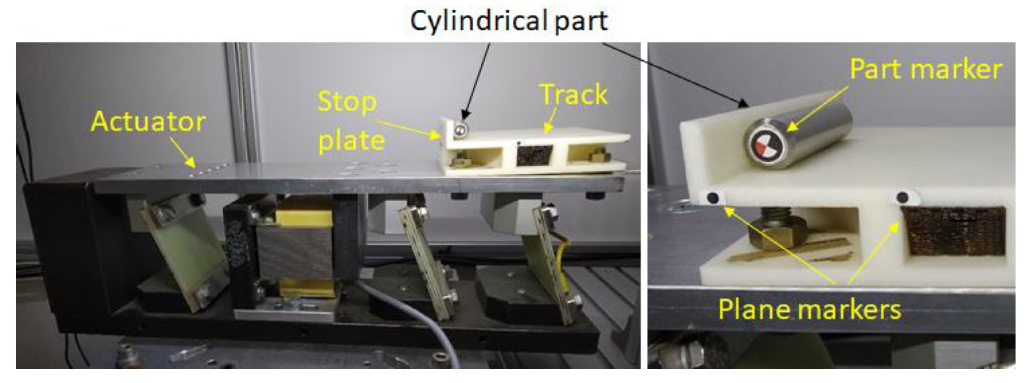
The paper is organized as follows. First, the dynamic equations governing the rolling motion of a cylindrical part are analytically derived, the differences between vibratory conveying of rolling and non-rolling parts are highlighted, and the parameters with the largest influence on the rolling motion are found. Then, a two-dimensional (2D) non-linear numerical model is developed that takes into account the transition between pure rolling and rolling with sliding and the impacts of the cylindrical parts with the edge of the conveyor. Series of numerical simulations are carried out, which show the effects of variations in the system’s parameters on the motion of the cylindrical part. Finally, testing equipment composed of a vibrating conveyor and a vision system that monitors the motion of a cylinder is presented. Numerical results are compared with experimental results, and the benefits and limits of 2D simulations are discussed.

2. Theoretical Basis

There are very important differences between the vibration conveying of parts that can roll on the conveyor track and parts that cannot roll. A 2D model with the plane of motion perpendicular to the axis of the cylinder is enough to point out these differences.

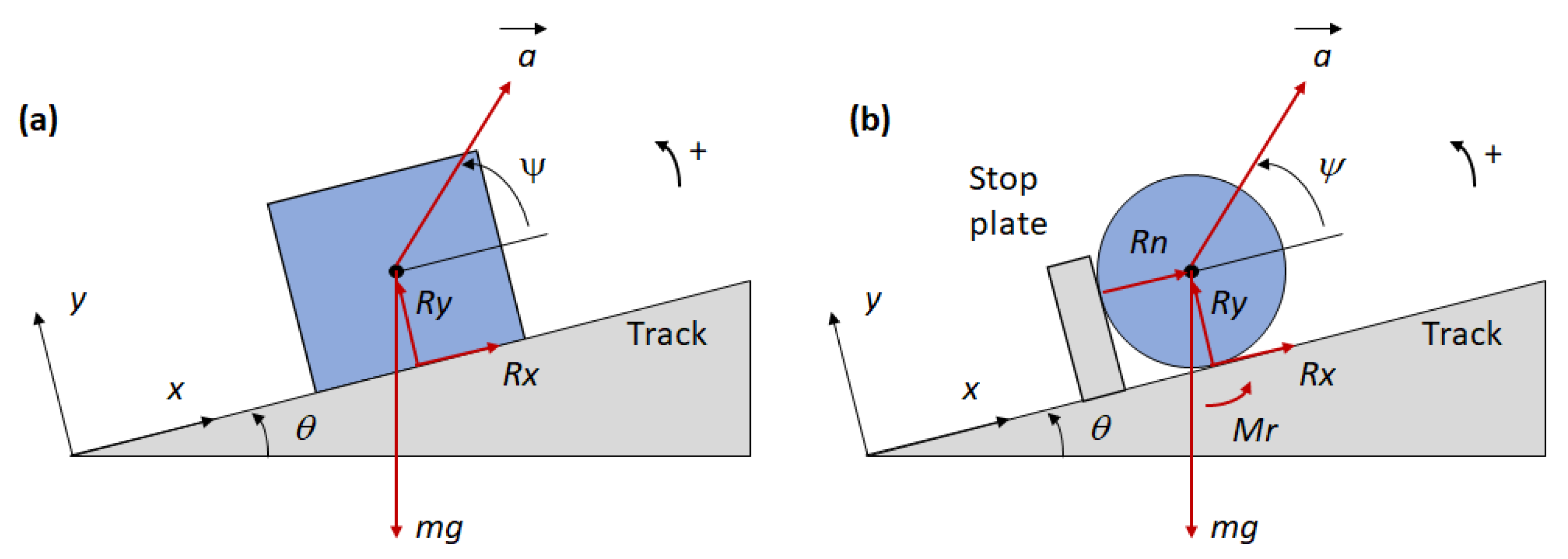
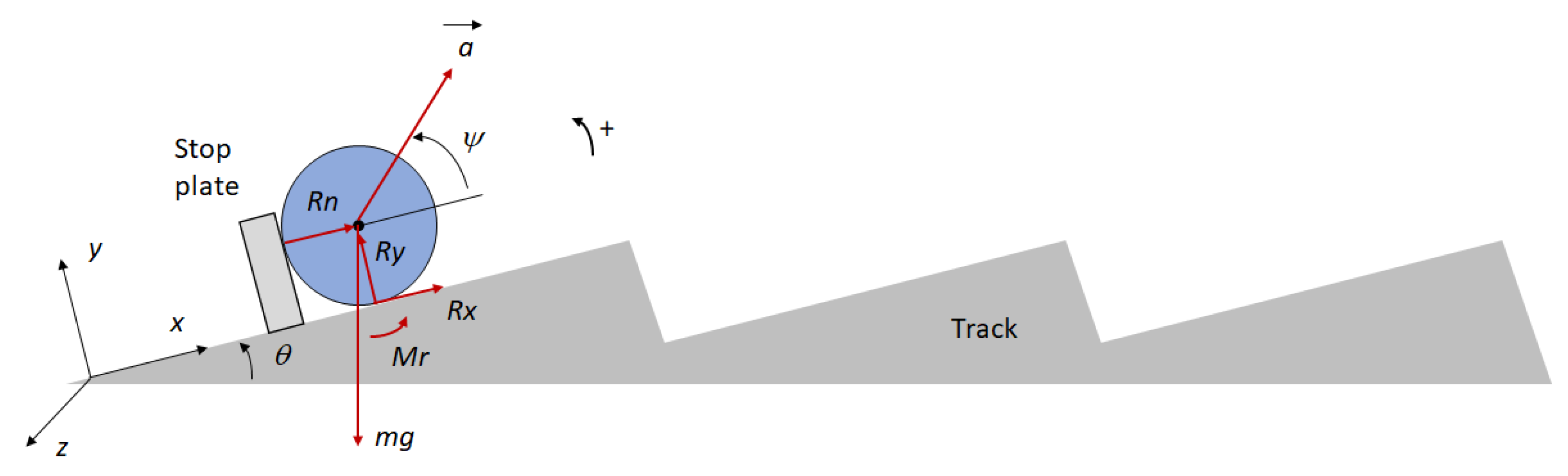
Vibration conveying of non-rolling parts is a dynamic phenomenon dominated by dry friction. Figure 1a shows a small block on the track of the conveyor, which is tilted by angle $\theta$ with respect to the horizontal direction. A fixed reference frame with axis $x$ parallel to the track and axis $y$ perpendicular to track is introduced. $R_x$ and $R_y$ are the components of the reaction force exerted by the track surface on the block (the positive direction is represented); they are related by the static Coulomb friction coefficient ${\mu }_s$ and by the kinetic Coulomb friction coefficient ${\mu }_c$. Acceleration ($\stackrel{\rightharpoonup }{a}$) of the conveyor is tilted by angle $\psi$ with respect to the conveyor track. If the motion of the conveyor is harmonic with amplitude $x_0$ and angular frequency $\omega$, the components of the acceleration are:

$$A_x=acos\left(\psi \right)=-x_0{\omega }^{2}sin\left(\omega t\right)cos\left(\psi \right)$$

(1)

$$A_y=asin\left(\psi \right)=-x_0{\omega }^{2}sin\left(\omega t\right)sin\left(\psi \right).$$

(2)

Angle $\psi$ is essential for the vibration conveying of non-rolling parts. When acceleration has the direction shown in Figure 1a, the inertia force adds to the weight of the block, the reaction force $R_y$ is large, the modulus of the demanded tangential reaction force |R_x| is smaller than the maximum static friction force (${\mu }_s\left|R_y\right|)$, and the block cannot slide backwards. Conversely, when acceleration $\stackrel{\rightharpoonup }{a}$ changes its direction, the inertia force tends to cancel the weight force, $R_y$ decreases, and the modulus of the demanded tangential reaction force $\left|R_x\right|$ may become larger than the maximum static friction force; hence, the block moves, and forwards sliding begins. This condition repeats at every period of the harmonic motion and eventually the block moves forwards with respect to the track.

The scenario drastically changes when the part has a cylindrical shape, as depicted in Figure 1b. A stop-plate is introduced, and $R_n$ is the reaction force exerted by the stop plate on the cylinder (the positive direction is represented), $M_r$ is the rolling resistance torque (the positive direction is represented), $m$ is the cylinder mass, and $mg$ is the gravity force (the actual direction is represented).

First, the cylindrical part is assumed to be steady on the vibrating conveyor, and the dynamic conditions that make possible the beginning of the relative motion are analyzed. The equations of motion in the $x$ and $y$ directions are:

$$m{a}_x=-mgsin\left(\theta \right)+ R_x+R_n$$

(3)

$$m{a}_y=-mgcos\left(\theta \right)+ R_y.$$

(4)

In Equations (3) and (4), $a_x$ and $a_y$ are the two components of the acceleration of the center of mass of the cylindrical part.

When there is no relative motion, $a_x$ and $a_y$ coincide with the components of acceleration of the conveyor ($A_x$ and $A_y$); therefore, the equations of motion become:

$$macos\left(\psi \right)=-mgsin\left(\theta \right)+ R_x+R_n$$

(5)

$$ma sin\left(\psi \right)=-mgcos\left(\theta \right)+ R_y.$$

(6)

The perpendicular reaction force con be calculated from Equation (6).

$$R_y= ma sin\left(\psi \right)+mgcos\left(\theta \right)$$

(7)

The contact between the cylinder and the track is unilateral; hence, $R_y\ge 0$. When $R_y$ tends to zero, the cylinder separates from the track, and the hopping motion begins. The hopping motion can be avoided decreasing the vibration acceleration, and this solution leads to a noise reduction [9]. Thus, this kind of motion is not considered in the framework of this research.

The angular momentum equation about the center of mass of the cylindrical part is:

$$I_G\ddot{\phi }=r R_x-u_{rs}{R}_{y}sgn\left(\dot{\phi }\right).$$

(8)

Reaction force $R_n$ does not appear in Equation (8), because it passes through the center of mass of the cylinder. $I_G$ is the moment of inertia about the center of mass, r is the cylinder radius, $u_{rs}$ is the coefficient of rolling resistance in static condition, $\ddot{\phi }$ is the angular acceleration, $\dot{\phi }$ is the angular velocity, and $sgn$ is the signum function. Since the beginning of the rolling motion is considered, $\ddot{\phi }=0$ and $sgn\left(\dot{\phi }\right)=-1$, because after the beginning of relative motion, a negative rolling velocity will take place: $\dot{\phi }=-v_r/R$. Tangential reaction force R_x can be calculated from the angular momentum equation:

$$R_x= -\frac{u_{rs}}{R}{R}_y.$$

(9)

The term $\frac{u_{rs}}{R}$ is the non-dimensional rolling friction coefficient in static condition, which is named $f_{vs}$.

The reaction force that the stop plate exerts on the cylinder ($R_n$) can be calculated from Equations (5) and (9). The contact between the cylinder and the stop plate is unilateral $\left(R_n>0\right)$. Hence, the condition $R_n\le 0$ in conjunction with the adoption of the maximum rolling friction coefficient in Equation (9) defines the beginning of the relative motion between the cylinder and the conveyor track:

$$R_n= macos\left(\psi \right)+mgsin\left(\theta \right)+ f_{vs}{R}_y\le 0,$$

(10)

If Equation (6) is introduced into Equation (10), the following condition for the beginning of rolling motion is obtained:

$$\frac{a}{g}\le -\frac{sin\left(\theta \right)+f_{vs}\mathit{cos}\left(\theta \right)}{cos\left(\psi \right)+f_{vs}sin\left(\psi \right)} .$$

(11)

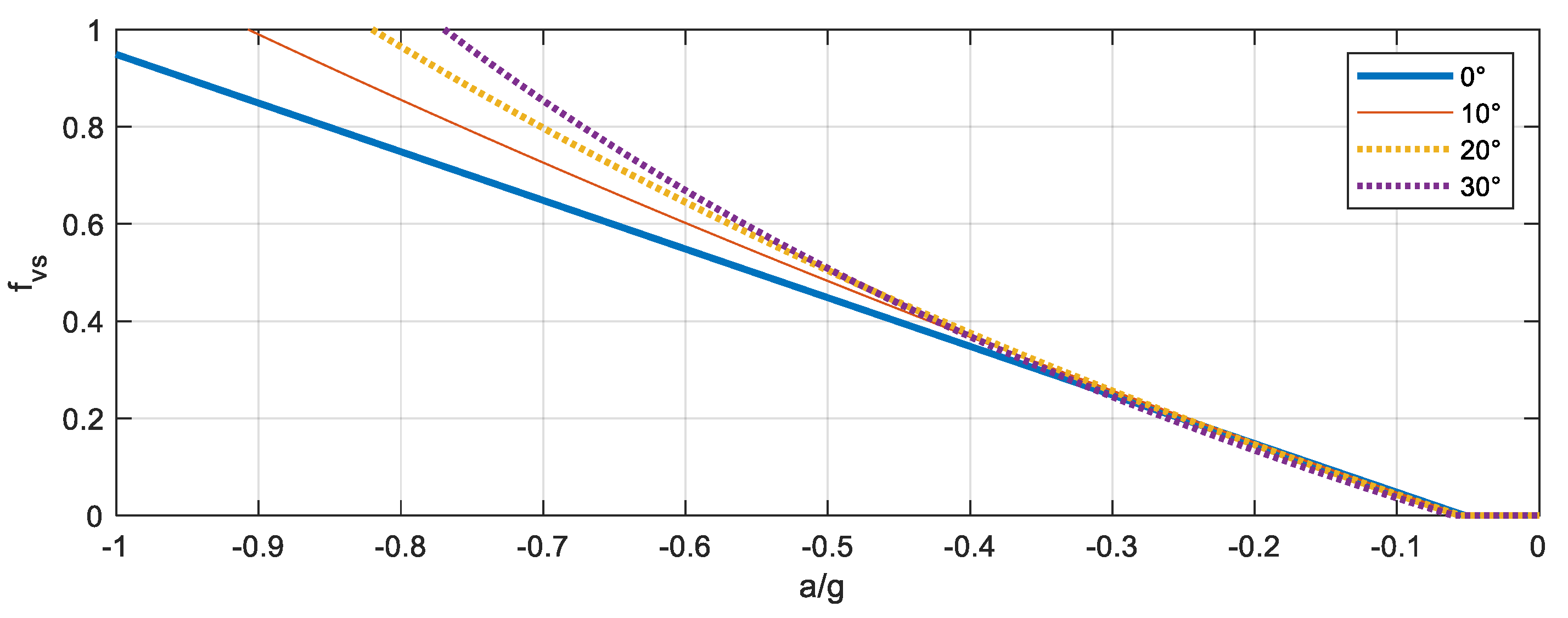
Figure 2 depicts the values of the static rolling friction coefficient ($f_{vs})$ that prevents the rolling motion against non-dimensional acceleration ($a/g$) for parametric values of $\psi$. Only negative values of acceleration are considered, since a negative acceleration is required to begin the rolling motion; the maximum value of non-dimensional acceleration is $a/g=-sin\left(\theta \right)/cos\left(\psi \right),$ since for larger values, the resultant of the gravity and inertia forces pushes the cylinder against the stop plate.

Figure 2 shows that very large and unrealistic values [16] of static rolling friction coefficient ($f_{vs}$) are needed to prevent the beginning of the rolling motion. When $a/g$ is lower than −0.35, the increase in angle $\psi$ increases the value of $f_{vs}$.

Hypothetically, the cylindrical part excited by conveyor vibrations could begin a sliding motion as well. The following condition for the beginning of the sliding motion can be derived:

$$\frac{a}{g}\le -\frac{sin\left(\theta \right)+{\mu }_{s}cos\left(\theta \right)}{cos\left(\psi \right)+{\mu }_{s}sin\left(\psi \right)} .$$

(12)

It is worth noticing that this condition is the same that holds true for non-cylindrical parts [1]. Equation (12) is similar to Equation (11), but $f_{vs}$ is substituted by μ_s, which is the static Coulomb friction coefficient. For most of the materials used in industrial applications [16], the static Coulomb friction coefficient is much larger than the non-dimensional rolling friction coefficient in static condition. Therefore, the negative acceleration needed to begin the sliding motion is much larger (in modulus) than the one needed to begin the rolling motion.

The evolution of the rolling motion is now analyzed. The equations of motion are:

$$m{a}_x=-mgsin\left(\theta \right)+ R_x$$

(13)

$$m{A}_y=-mgcos\left(\theta \right)+ R_y$$

(14)

$$I_G\ddot{\phi }=r R_x-f_{v}R{R}_{y}sgn\left(\dot{\phi }\right).$$

(15)

Moreover, during pure rolling, the following kinematic condition has to be fulfilled:

$$\ddot{\phi }=-\frac{a_x-acos\left(\psi \right)}{R}.$$

(16)

$R_y$ can be calculated from Equation (14); then, Equations (13), (15), and (16) can be solved to calculate $R_x$, $a_x$, and $\ddot{\phi }$. Taking into account that for a cylinder $I_G=0.5m{R}^2$, the following results are obtained:

$$R_x=\frac{1}{3} m\left(acos\left(\psi \right)+gsin\left(\theta \right)\right)+\frac{2}{3}{f}_v{R}_{y}sgn\left(\dot{\phi }\right)$$

(17)

$$a_x=\frac{1}{3} acos\left(\psi \right)-\frac{2}{3}gsin\left(\theta \right)+\frac{2}{3}{f}_v\frac{R_y}{m}sgn\left(\dot{\phi }\right)$$

(18)

$$\ddot{\phi }=-\frac{1}{R}\frac{2}{3}\left(-acos\left(\psi \right)-gsin\left(\theta \right)+f_v\frac{R_y}{m}sgn\left(\dot{\phi }\right)\right).$$

(19)

It is worth noticing that when the cylinder rolls forwards ($\dot{\phi }<0$), the rolling friction term in Equation (19) adds to the gravity term. The motion of the cylinder on the conveyor track can be studied integrating Equations (18) and (19); the input is acos(ψ). Generally speaking, a numerical integration is needed (see Section 3) owing to the $sgn$ function. Nevertheless, $f_v<0.01$ in most industrial processes, and an approximation of the integrals of Equations (18) and (19) can be obtained assuming $f_v=0$.

According to Equation (11), the forward motion begins when $a/g\le -sin\left(\theta \right)/cos\left(\psi \right)$. Since in normal conveying applications angle $\theta$ is rather small, another simplification can be made assuming that the forward rolling motion begins when $acos\left(\psi \right)=-x_0{\omega }^{2}sin\left(\omega t\right)cos\left(\psi \right)$ becomes negative. This assumption simplifies the initial conditions, because in the harmonic motion vibration, the acceleration changes its sign when the displacement is zero and the velocity has the maximum positive value (x₀ω).

The integration of Equation (18) with the above-mentioned simplifications and initial conditions leads to the following equations for the absolute velocity ($v_x$) and displacement ($x$) of the center of mass of the cylinder:

$$v_x=\frac{1}{3} \omega x_0\mathit{cos}\left(\omega t\right)cos\left(\psi \right)+\frac{2}{3} \omega x_{0}cos\left(\psi \right)-\frac{2}{3}gsin\left(\theta \right)t$$

(20)

$$x=\frac{1}{3}{x}_0\mathit{sin}\left(\omega t\right)cos\left(\psi \right)+\frac{2}{3} \omega x_{0}cos\left(\psi \right)-\frac{1}{3}gsin\left(\theta \right)t^2.$$

(21)

From the point of view of conveying, the most important parameter is the relative velocity $v_r$ between the part and the track of the conveyor:

$$v_r=v_x- \omega x_0\mathit{cos}\left(\omega t\right)cos\left(\psi \right)$$

(22)

$$v_r=\frac{2}{3} \omega x_{0}cos\left(\psi \right)-\frac{2}{3} \omega x_0\mathit{cos}\left(\omega t\right)cos\left(\psi \right)-\frac{2}{3}gsin\left(\theta \right)t.$$

(23)

The relative velocity includes a positive and constant term due to initial velocity ($x_0\omega$); a harmonic term due to the vibration of the conveyor plate, whose integral over a period ($T=2\pi /\omega$) is zero; and a negative term due to gravity that increases (in modulus) with time.

If $\theta =0$ (horizontal conveying), the average conveying velocity in the period (${\tilde{v}}_r$) is constant and equal to $\frac{2}{3} \omega x_{0}cos\left(\psi \right)$. If $\theta >0$ the average conveying velocity decreases, and at the nth period it assumes the value:

$${\tilde{v}}_r=\frac{2}{3} \left(\omega x_{0}cos\left(\psi \right)-gsin\left(\theta \right)\frac{\pi }{\omega }\left(2n-1\right)\right) n=1,2, \dots N.$$

(24)

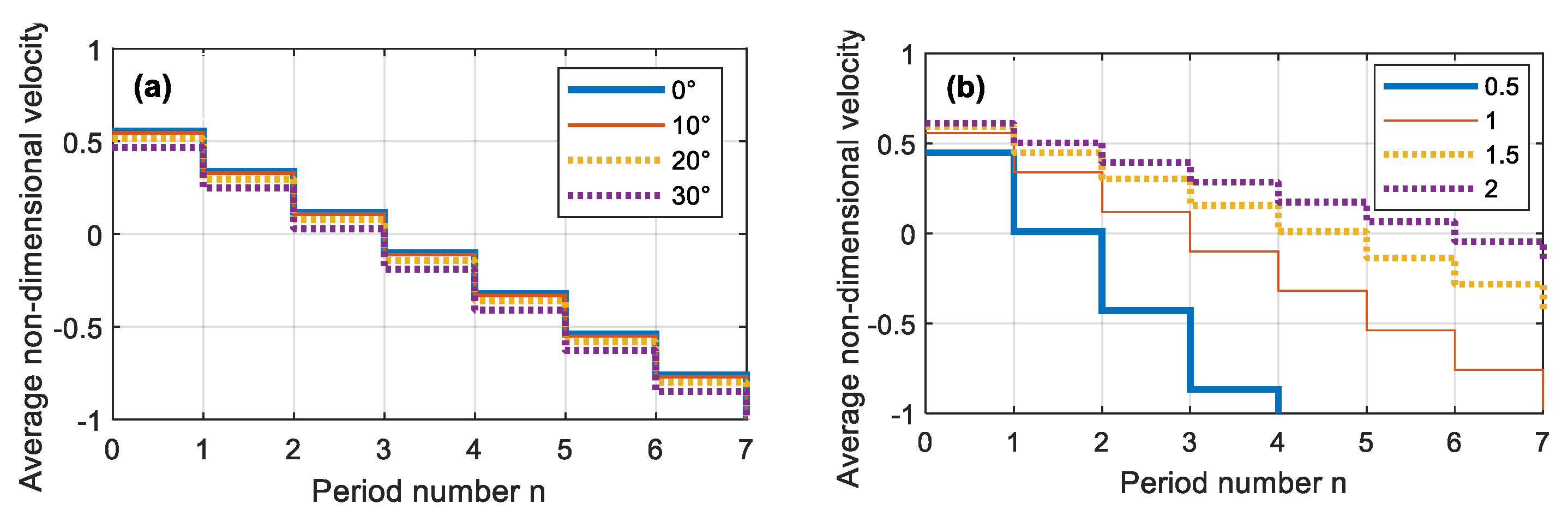
When ${\tilde{v}}_r$ becomes negative, the cylindrical part rolls backwards and eventually impacts the stop plate. Figure 3 depicts the ratio between ${\tilde{v}}_r$ and the maximum vibration speed ($x_0\omega$) versus period number ($n$) for θ = 3°. In Figure 3a, the ratio between the vibration acceleration and gravity acceleration ($a/g$) is 1 and the parametric values of angle $\psi$ are considered; the increase in ψ has a negative effect on the conveying speed. In Figure 3b, ψ is set to zero, and the parametric values of the ratio a/g are considered; the increase in vibration acceleration has a positive effect on vibration conveying.

Equation (24) holds true with the assumption $f_v=0$. If rolling resistance is present, it contributes to decreasing the average conveying speed in the period.

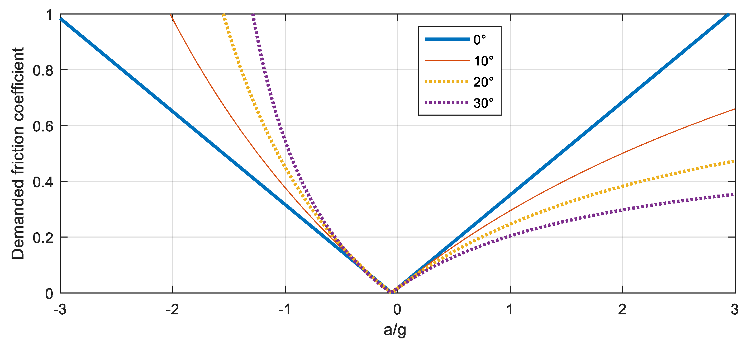
During pure rolling motion, the reaction force $R_x$ given by Equation (17) is needed to guarantee equilibrium. $\left|R_x\right|$ has to be smaller than the maximum static friction force (${\mu }_s{R}_y$). Hence, the ratio $\left|R_x\right|/R_y$ has the meaning of static friction coefficient needed to guarantee equilibrium during pure rolling. Figure 4 shows the ratio $\left|R_x\right|/R_y$ against non-dimensional acceleration ($a/g$) for $\theta =3°,f_v=0$ and parametric values of $\psi$.

With $\psi =0$, the friction coefficient needed to guarantee the pure rolling motion is only slightly influenced by the versus of acceleration.

With $\psi >0$, the friction coefficient needed to guarantee the pure rolling motion is significantly smaller when the conveyor acceleration is positive than when acceleration is negative. This phenomenon happens because when acceleration changes sign, the decrease in reaction force $R_y$ (Equation (7)) is not compensated by the decrease in $R_x$ (Equation (17)), and this effect becomes even more important when $\psi$ is large. Since in most industrial material ${\mu }_s$ is in the range of 0.6 ÷ 1 [1], the transition from a pure rolling motion to a rolling with sliding can take place only in the presence of large negative accelerations of the vibration conveyor.

When the cylindrical part rolls backwards, it may impact the stop plate; in this case, the equation of motion in the x direction becomes:

$$m{a}_x=-mgsin\left(\theta \right)+ R_x+F_{imp}$$

(25)

in which $F_{imp}$ is the impact force, which has the same direction of $R_n$ in Figure 1. $F_{imp}$ strongly increases $R_x$; hence, the ratio $\left|R_x\right|$/$R_y$ may reach very large values, and the sliding motion can begin.

3. Numerical Model

The simulation of the motion of a cylindrical part on a vibrating plane is not a simple task due to the non-linear phenomena that take place, e.g., the frequent transition between states of motion and the impacts with the stop plate. In order to address the problem, a combination of a MATLAB (R2019b, MathWorks Inc., Natick, MA, USA, 2020) script and its simulation environment Simulink was adopted. The simulations are started from a main MATLAB script which initializes the variables at the initial conditions: the cylinder is touching the track and in contact with the stop plate, as depicted in Figure 1b. The cylinder is supposed to start with a pure rolling motion; therefore, the main script launches a Simulink simulation, which implements this case. When a proper dynamic condition is met, the simulation is stopped and the simulation of rolling with sliding motion is started by the main script. Such simulation is stopped when particular kinematic and dynamic conditions are met. The process is iterated until the desired simulation duration is reached.

The block diagram of the simulation is represented in Figure 5. The two transition conditions require special attention, because they rule the simulation. The transition from pure rolling to rolling with sliding is ruled by a dynamic condition. When the tangential reaction force $R_x$ needed to guarantee the equilibrium of the pure rolling motion (Equation (17)) is larger than the maximum static friction force, the MATLAB main script stops the Simulink rolling model and starts the Simulink sliding model.

The MATLAB main script stops the Simulink sliding model when a dynamic and a kinematic condition are satisfied at the same time. The kinematic condition is the pure rolling condition, which is given by Equation (26).

$$v_x-V_x=-\dot{\phi }·R$$

(26)

This equation shows when there is a possible switching from rolling with sliding to pure rolling, but a dynamic condition is to be satisfied as well. This condition states that the tangential reaction force has to be smaller than the maximum static friction force.

One of the novelties of this numerical model with respect to previous papers [15] is the introduction of the impacts with the stop plate, which makes the integration of the equations more complex. Impact forces are calculated representing contact stiffness by means of a lumped spring, which is compressed only if the distance between the cylinder and the stop plate is smaller than a fixed threshold. For this reason, the simulation environment Simulink was chosen, which proved to be very intuitive for the integration of single sets of equations. Then, the problem was moved to the transition between the two cases. The development of a model entirely programmed in Simulink showed problems of flickering between different states and was not very effective. Therefore, it was decided to exploit the versatility of a simulation managed by a MATLAB script at the highest level with the power of the Simulink simulation environment at a lower level. The results lived up to expectations, although troubleshooting and a fine tuning of the parameters of the Simulink solver was needed.

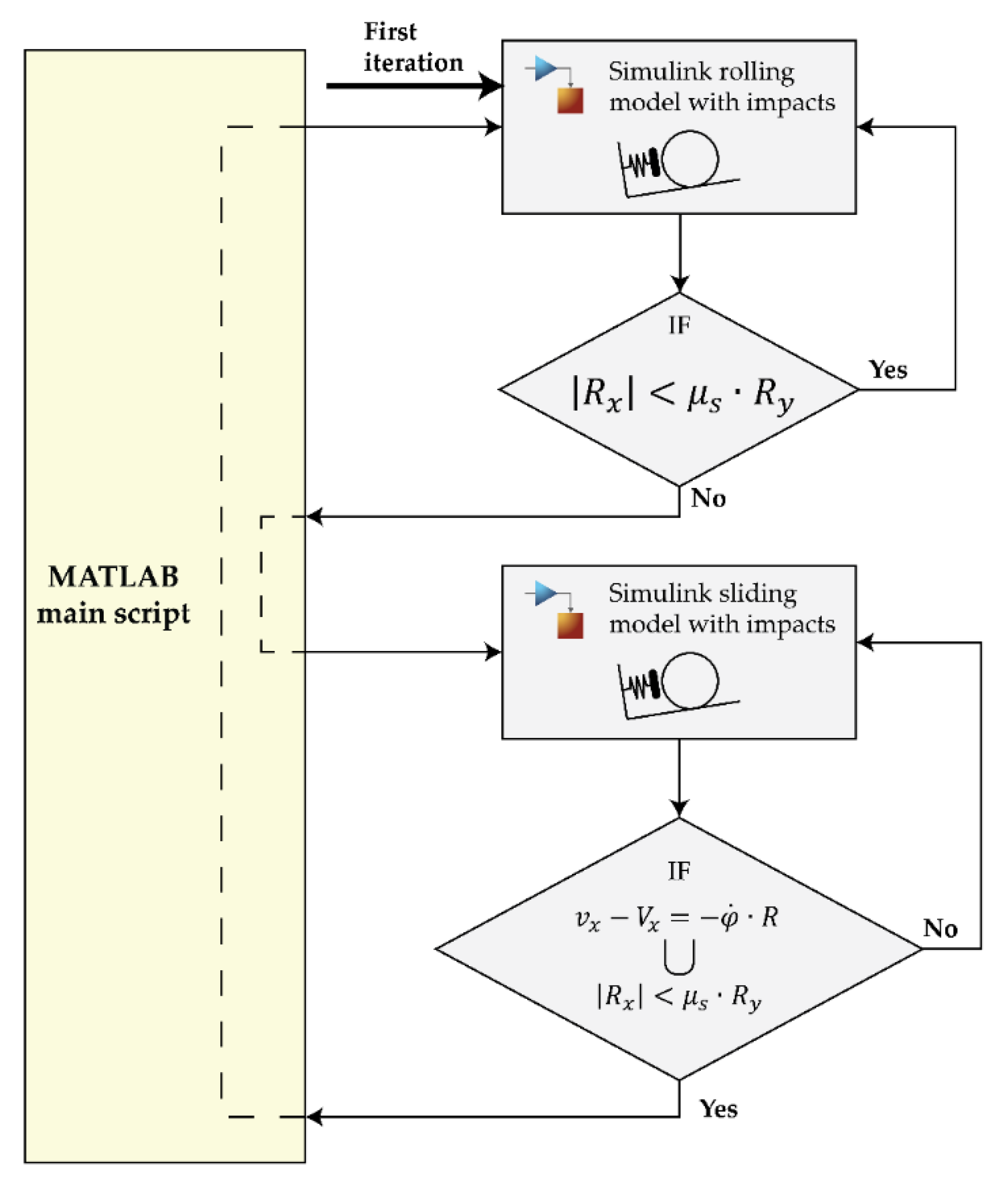
4. Numerical Results

Numerical simulations aimed at exploring the dynamics of vibration conveying of cylindrical parts beyond the limits of the analytical model of Section 2. In particular, numerical simulations made it possible to analyze the effect of the impacts of the cylindrical part on the stop plate.

A realistic reference case was defined, which is characterized by the following parameters of the vibratory conveyor: $x_0$= 0.0002 m, $\omega =$ 314 rad/s (frequency 50 Hz), $\theta =$ 3°, $\psi =$ 0°. The maximum modulus of conveyor acceleration is 19.72 m/s² $(a/g=2$).

The rolling part has a radius $r=$0.007 m and mass $m=$ 0.096 kg. The friction parameters are $f_v=$ 0.005, ${\mu }_c=0.3$, and ${\mu }_s=0.6$. The value of the rolling resistance is more than twice that of the typical rolling elements of bearings [16] and takes into account that the cylindrical part may be rough or dirty. The kinetic Coulomb friction coefficient value is inside the typical range of values found in vibratory conveyors [1,6,9]. The static Coulomb friction coefficient was set to be twice the kinetic coefficient [17]. Finally, the impact stiffness was set to $k=1,000,000$ N/m; this value made it possible to obtain values of contact forces similar to the measured ones (about 60 ÷ 80 N).

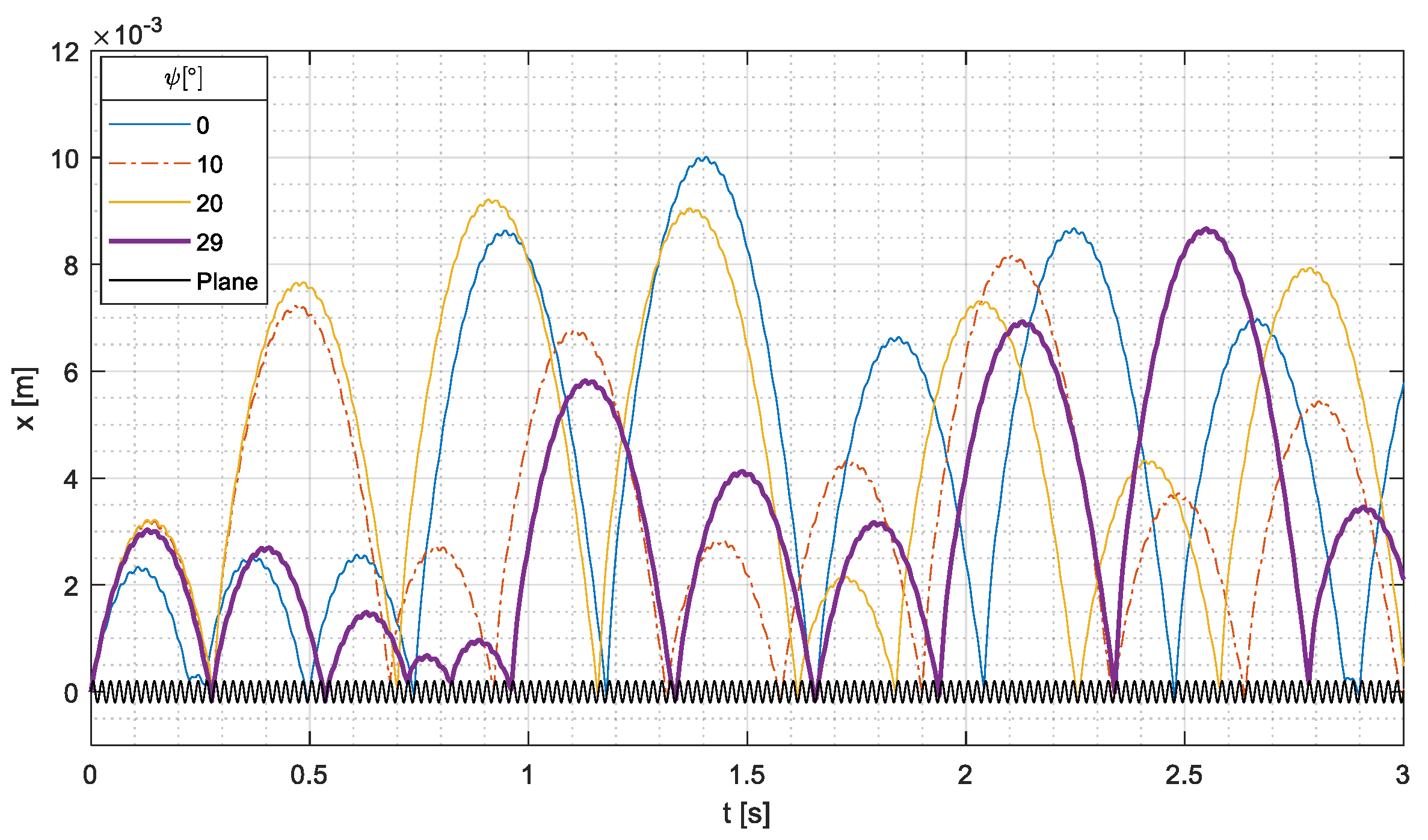
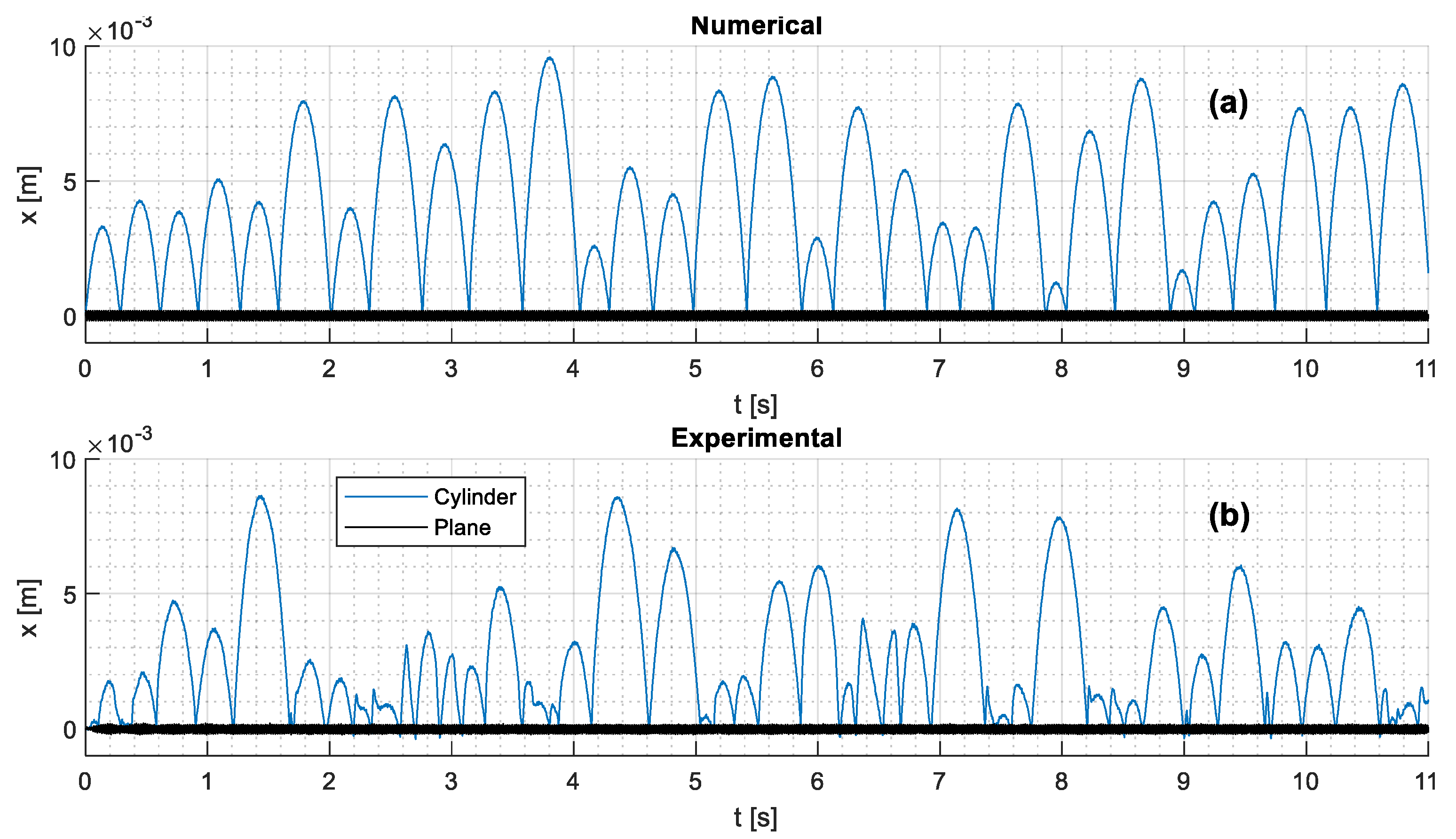
The first parametric simulations aimed at analyzing the effect of angle $\psi$; Figure 6 shows numerical results in terms of the absolute displacement of the cylinder center of the mass. In the same figure, for comparison, the displacement of the conveyor is represented (along the direction tilted by $\psi$ with respect to the $x$ axis).

In the plots of Figure 6, two different phases can be identified. The first phase (phase 1), which ends at about 0.25 s and includes 10 $÷12$ vibration periods, is the initial motion of the cylindrical part without impacts. As foreseen by theoretical analysis, the cylindrical parts begins its motion at $t=0$ owing to the initial velocity given by the conveyor, reaches the maximum displacement, and eventually impacts the stop plate. The maximum displacement is rather small (about 0.003 m), and this value is in agreement with the theoretical predictions (Equation (21)).

In this phase, the increase in the angle $\psi$ up to 20° leads to an increase in the traveled distance, a further increase leads to a reduction in the traveled distance. This particular behavior is due by the presence of two opposite effects.

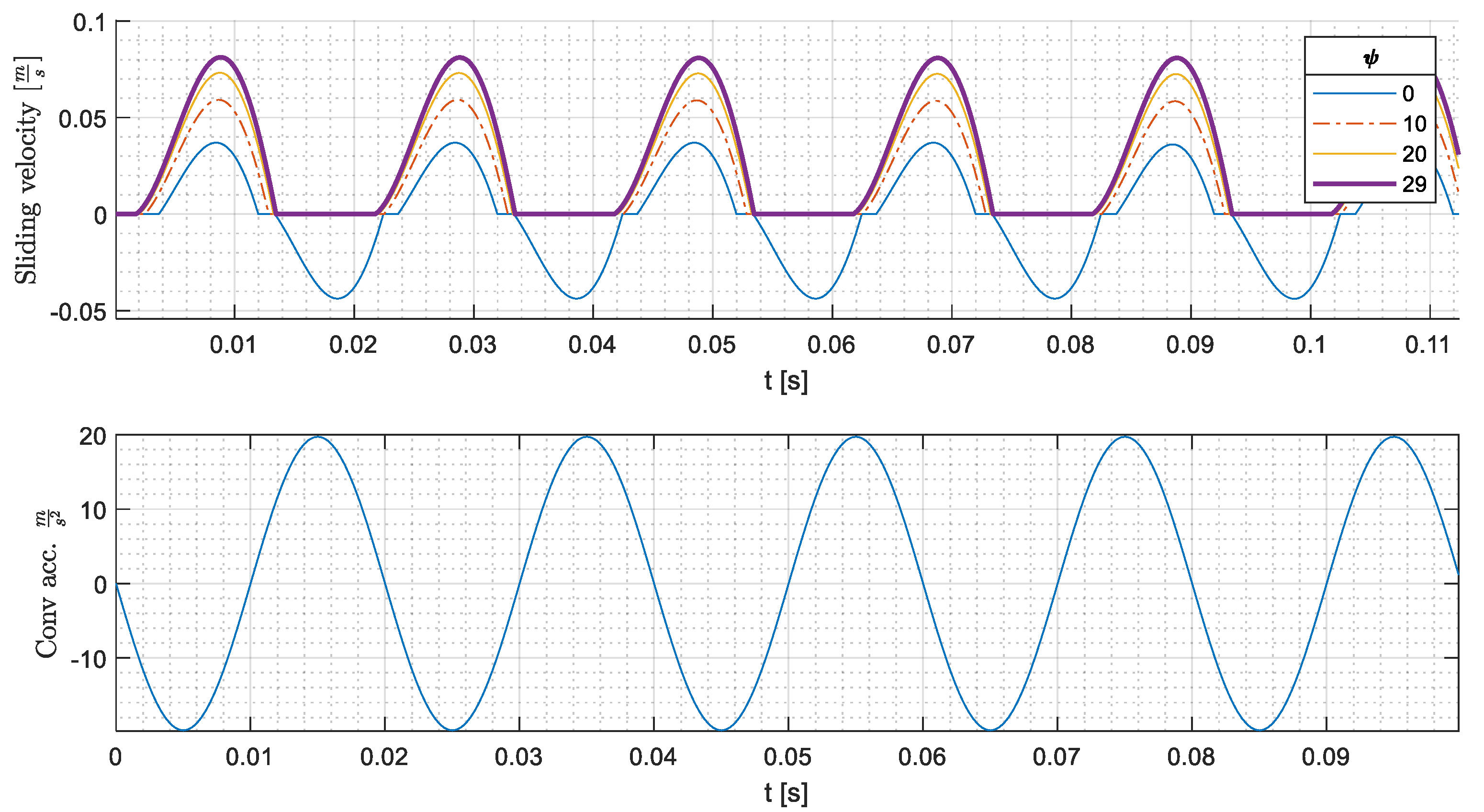
The first effect can be understood looking at the sliding velocity ($v_{sl}$) of the cylindrical part:

$$v_{sl}=v_x-V_x+R\dot{\phi }$$

(27)

which is plotted in Figure 7 with conveyor acceleration. If $\psi =0$, the cylindrical part slides both when the conveyor acceleration is negative and positive (forwards and backwards sliding, respectively). Backwards sliding causes a reduction in the traveled distance. This phenomenon is in agreement with the analytical results of Figure 4, which show that for $\psi =0$, the static friction coefficient needed to guarantee the pure rolling motion is larger than ${\mu }_s=0.6$ both for negative (−2) and for positive (+2) values of non-dimensional acceleration.

Conversely, Figure 7 shows that if $\psi$ increases, there is only forwards sliding, since the static friction coefficient is able to prevent backwards sliding when the conveyor acceleration becomes positive, and the cylindrical part behaves similar to a block. It is worth noticing that this behavior is in agreement with the analytical results of Figure 4.

The second effect is the decrease in the initial velocity of the cylindrical part when $\psi$ increases; see Equation (20). In summary, for small values of $\psi$, the first effect is dominant, and the traveled distance increases, whereas for large values of $\psi$, the second effect reduces the traveled distance.

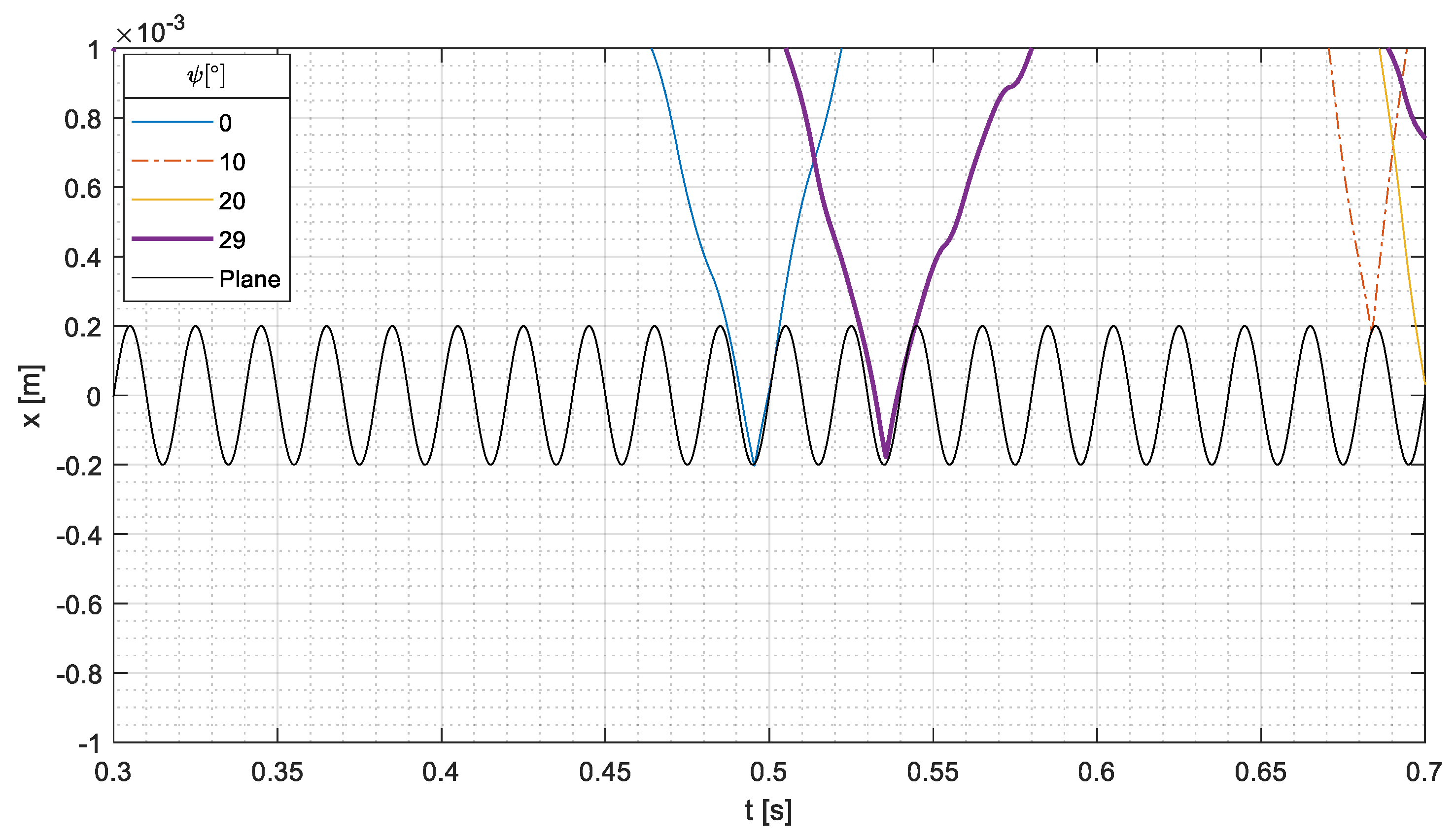
The second phase of the motion (phase 2, $t>$0.25 s) is dominated by the impacts of the cylindrical part on the stop plate.

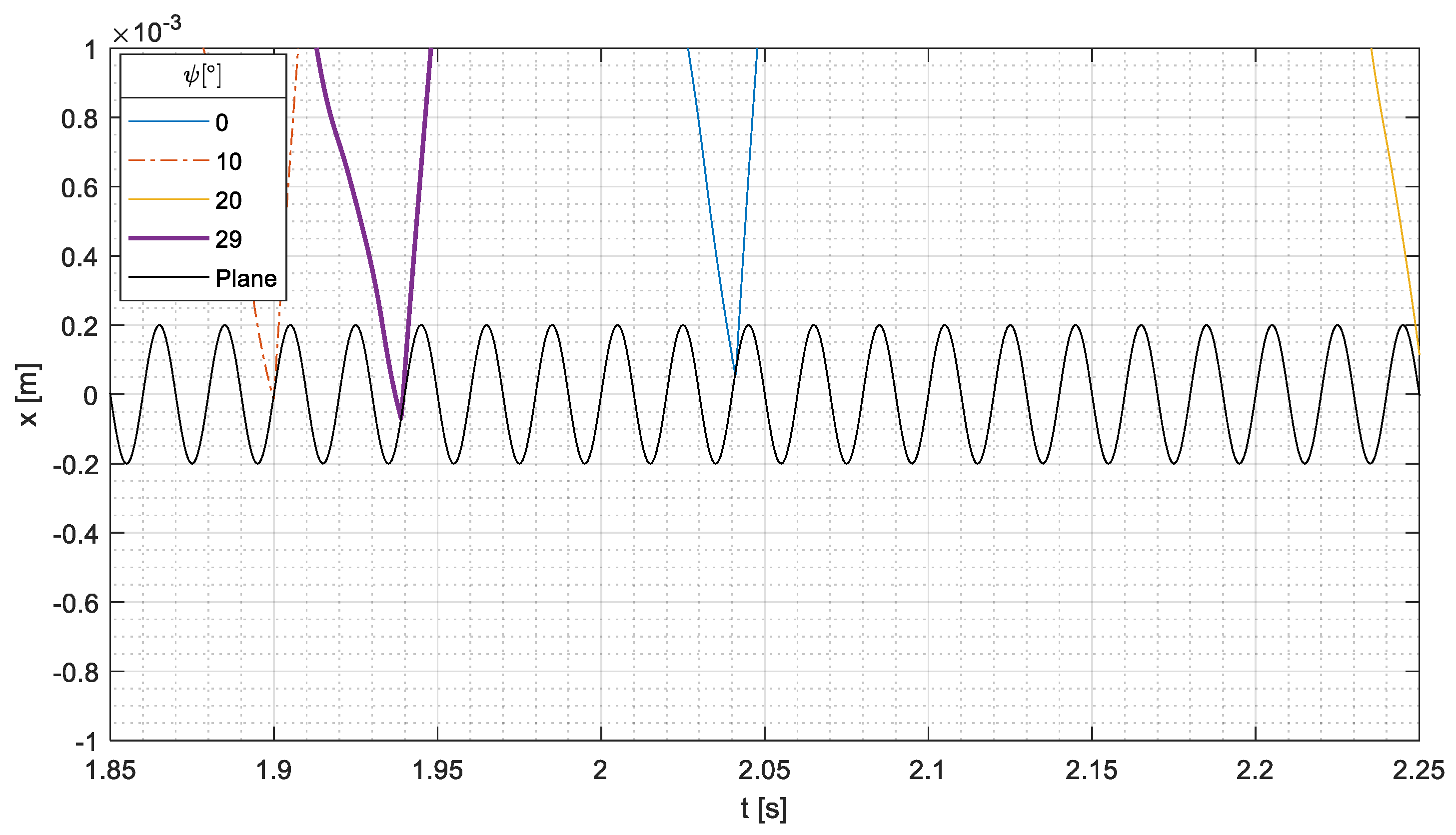
The cylindrical part reaches the maximum displacement in this phase, and this value chiefly depends on impact mechanics. If the relative velocity (Equation (22)) is large, because the cylindrical part and the conveyor move in opposition, the conveyor transfers a lot of energy to the cylindrical part, which has a large rebound after the impact. This phenomenon occurs at $t=2.04$ for $\psi =0°$. Figure 8, which is a zoom of Figure 6 of about $t=2.04 s$, shows that the impact occurs when the conveyor has the maximum positive velocity, whereas the velocity of the cylindrical part is negative. Conversely, if the relative velocity is small, because the cylindrical part and the conveyor move in phase, the conveyor transfers less energy to the cylindrical part, and a smaller rebound occurs. This phenomenon takes place at $t=0.49 \mathrm{s}$ for $\psi =0°$, since Figure 9 shows that the cylindrical part impacts the conveyor when it has a negative velocity.

The angle of conveyor acceleration ($\psi$) has a negligible effect on the second phase (impact dominated) of the motion of the cylindrical part on the conveyor, since the relative velocity at the impact depends much more on the previous motion than on conveyor maximum velocity, which slightly decreases if $\psi$ increases. Actually, after some impacts, the relative velocity at the impact changes randomly. Thus, the motion of the cylindrical part on the conveyor is similar to the motion of a bouncing ball that impacts a vibrating table, which may exhibit a chaotic behavior [18,19].

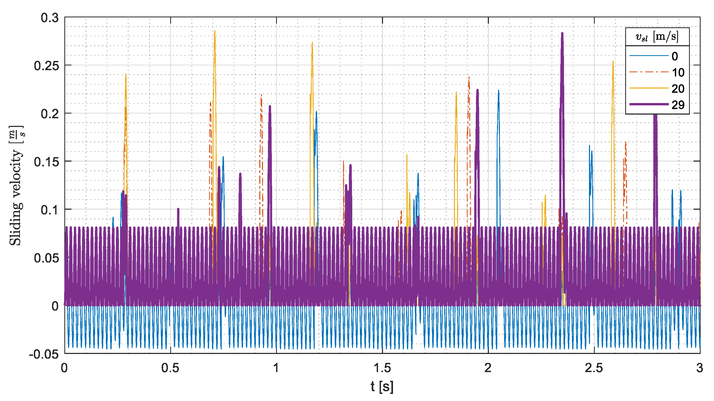
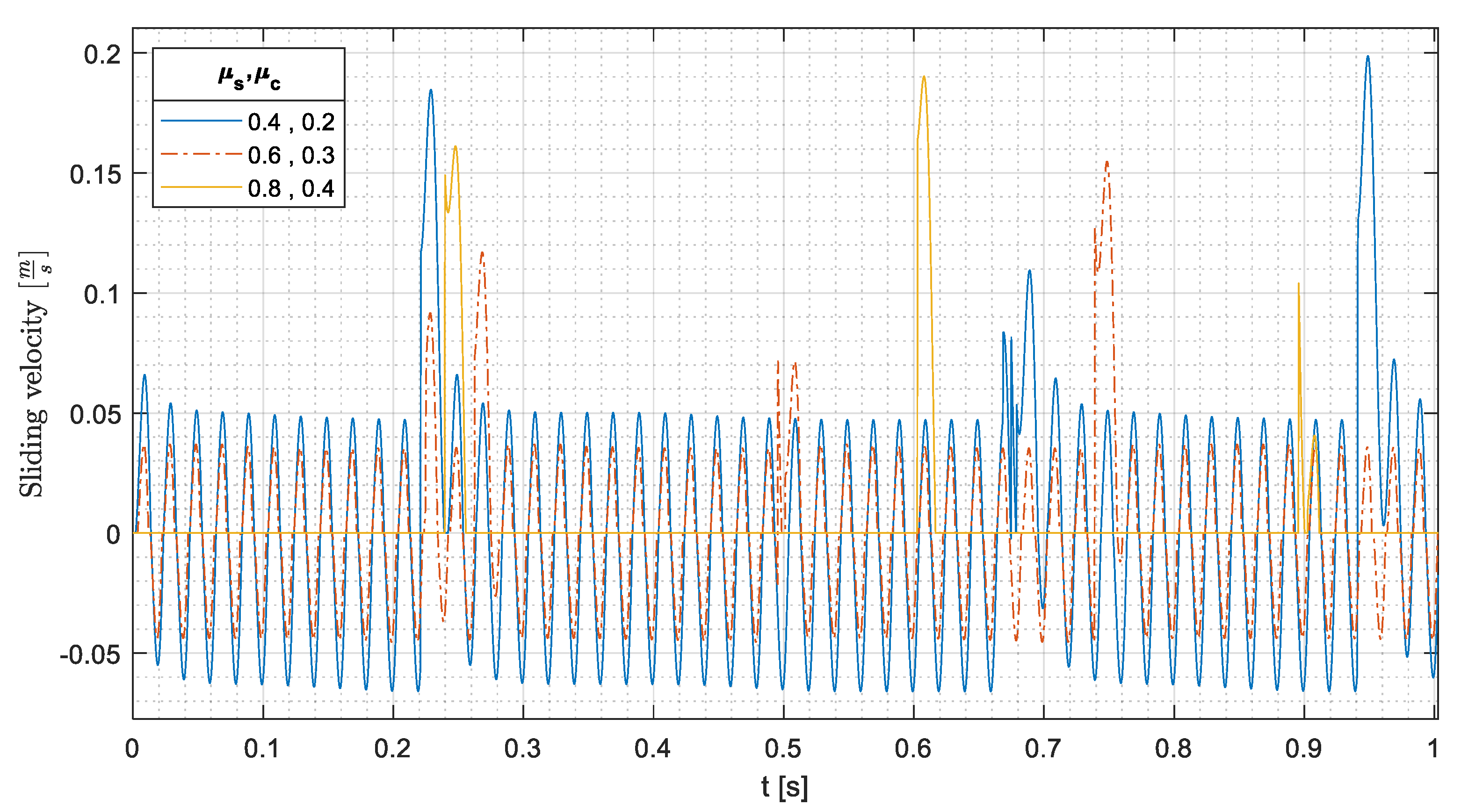
Figure 10 shows for the same cases of Figure 6 the sliding velocity of the cylindrical part and highlights that, owing to the large value of non-dimensional acceleration ($a/g =$ 2), very often the cylinder slides on the conveyor track. The largest sliding velocities take place just after the impacts.

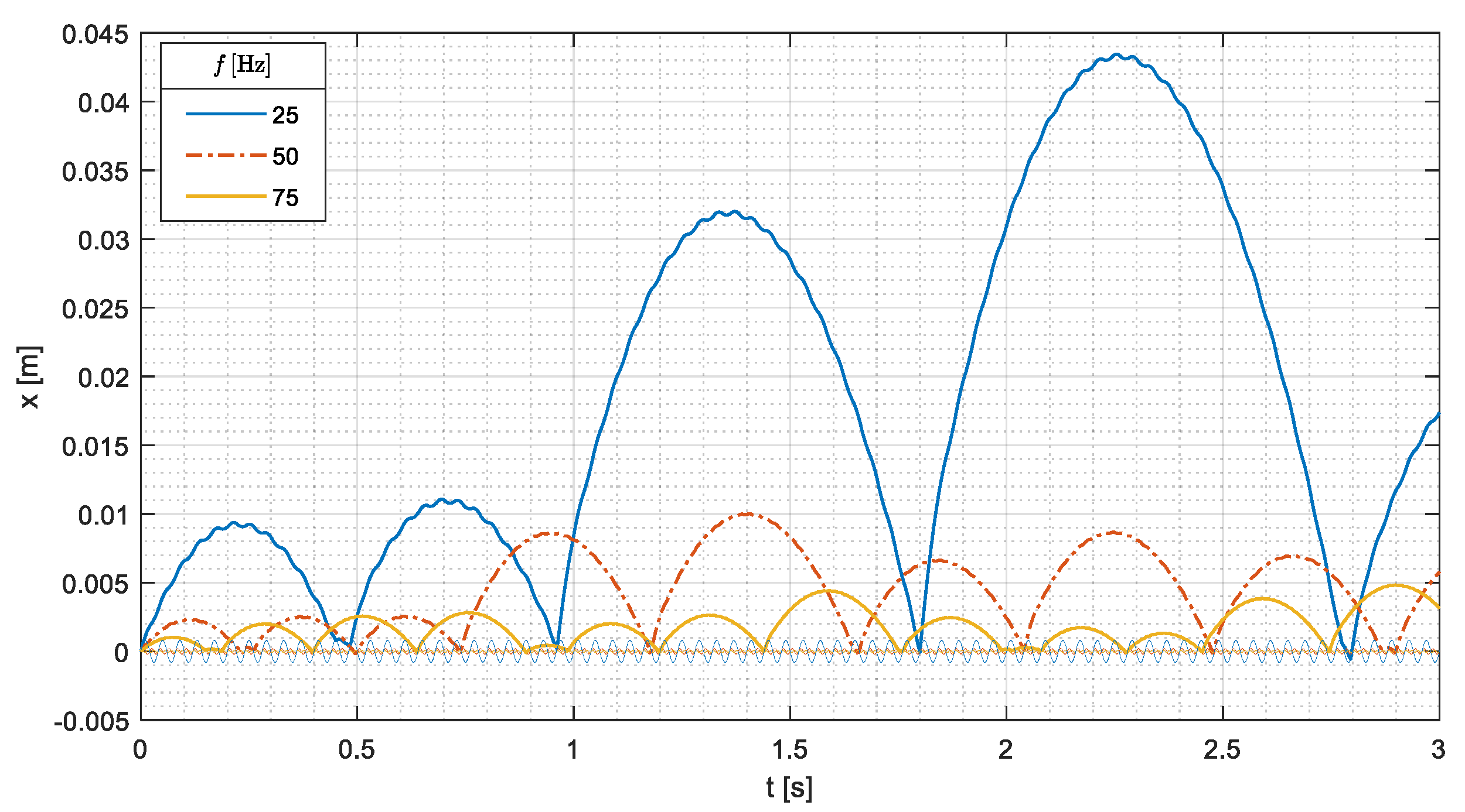
The second parametric simulation aimed at analyzing the effect of conveyor vibration frequency. Conveyor acceleration was kept equal to the previous value ($a/g =$ 2); therefore, an increase in frequency led to a decrease in velocity according to this equation:

$$v=\frac{a}{\omega }.$$

(28)

Figure 11 clearly shows that the increase in the frequency has a negative effect on the motion of the cylindrical part both before and after the first impact. The first effect takes place because the initial velocity is smaller, while the second effect takes place because the relative velocity at the impact is smaller. If the vibration frequency decreases to 25 Hz, the traveled distance increases up to 0.043 m. It is worth noticing that even if the dynamics of conveying of block-shaped parts and cylindrical parts are very different, the decrease in vibration frequency has a positive effect in both cases [1].

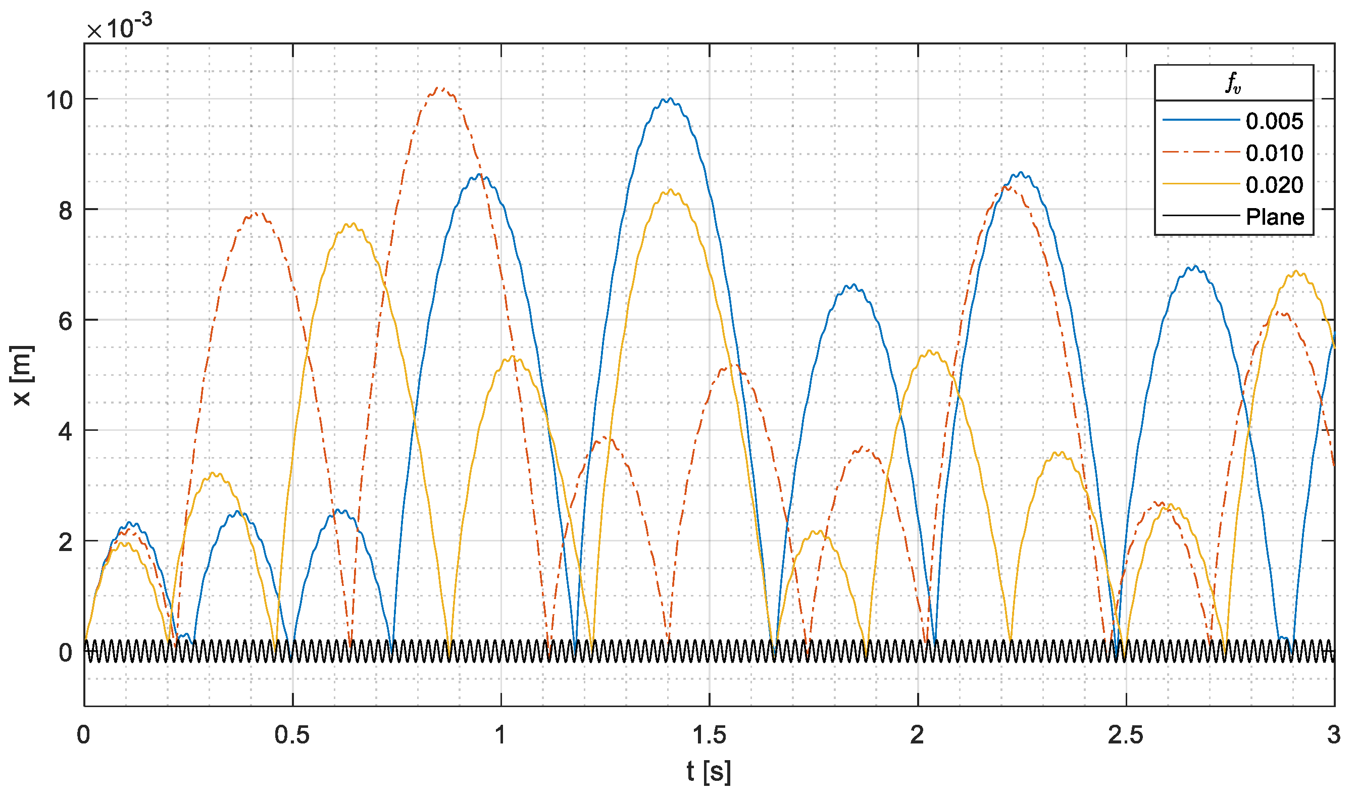
Then, the effect of rolling friction coefficient was investigated by means of numerical simulations. The results, which are presented in Figure 12, show that realistic variations in $f_v$ have a negligible effect on the conveying of cylindrical parts. Before the first impact (phase 1), the decrease in $f_v$ causes a very small increase in the traveled distance. After the first impact (phase 2), the variation in the rolling friction coefficient changes the instants in which the most energetic impacts take place, but the traveled distance does not significantly change.

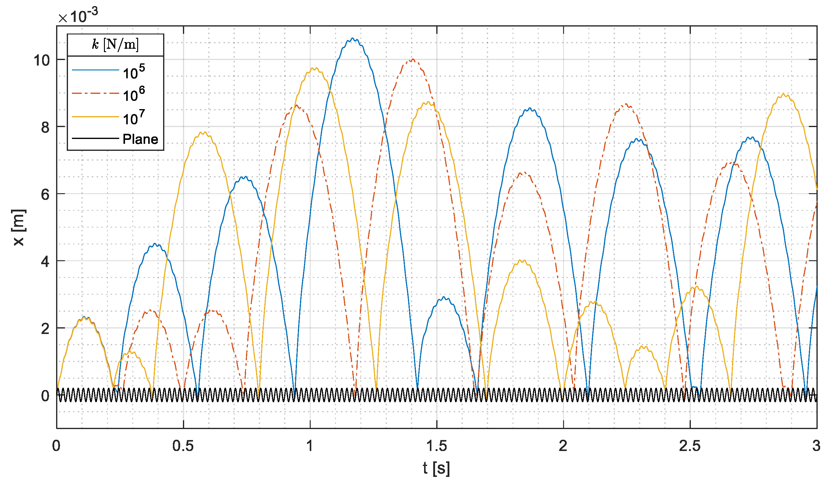
Figure 13 shows the effect of contact stiffness on the conveying of cylindrical parts. The contact stiffness does not affect phase 1, and it does not have a clear effect on the traveled distance in phase 2. This phenomenon agrees with physical intuition, because the contact stiffness is another factor that contributes to randomly varying the relative velocity at the impact, which is the main factor influencing the rebound of the cylindrical part.

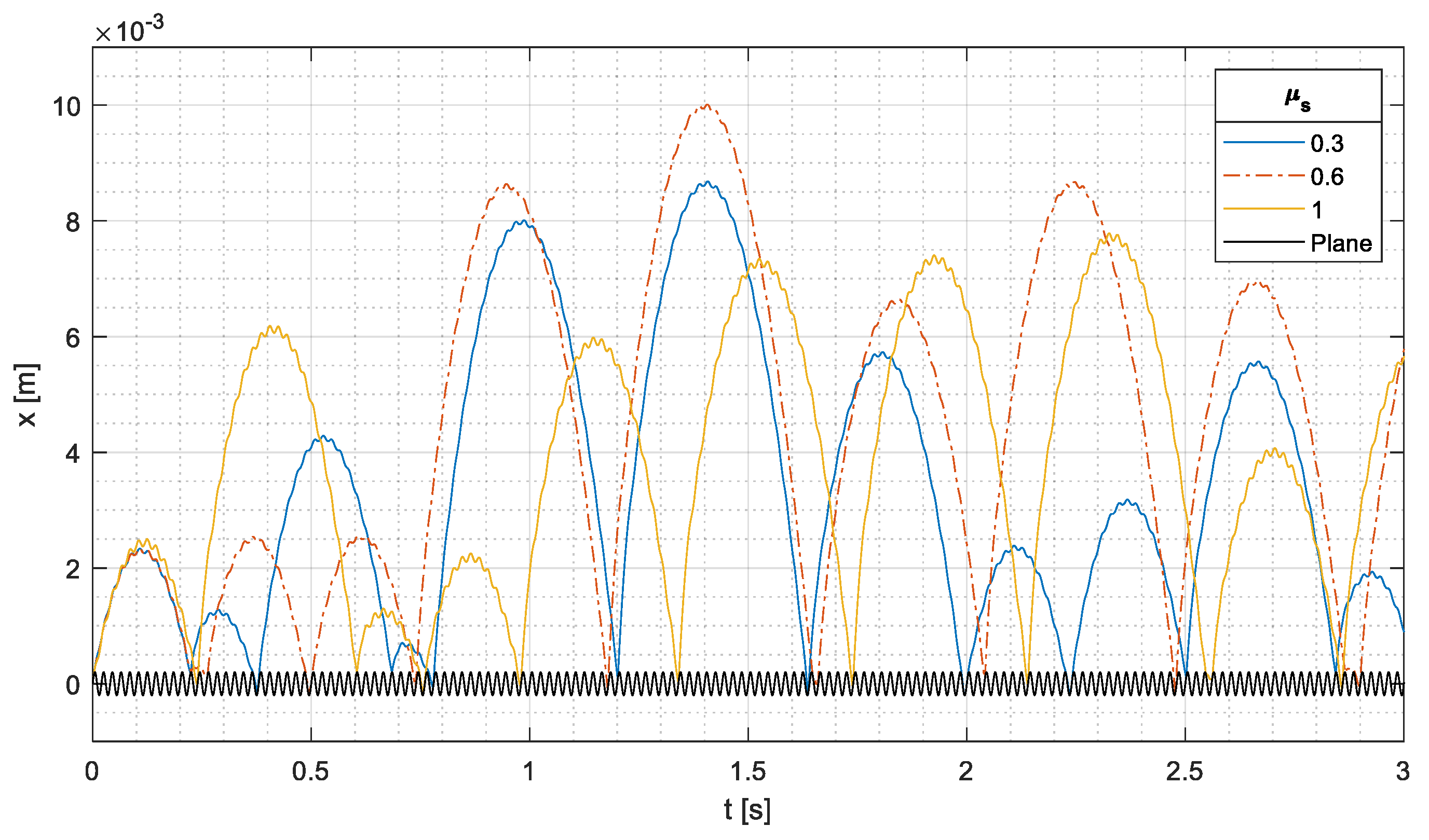
Finally, the effect of friction coefficients was investigated.

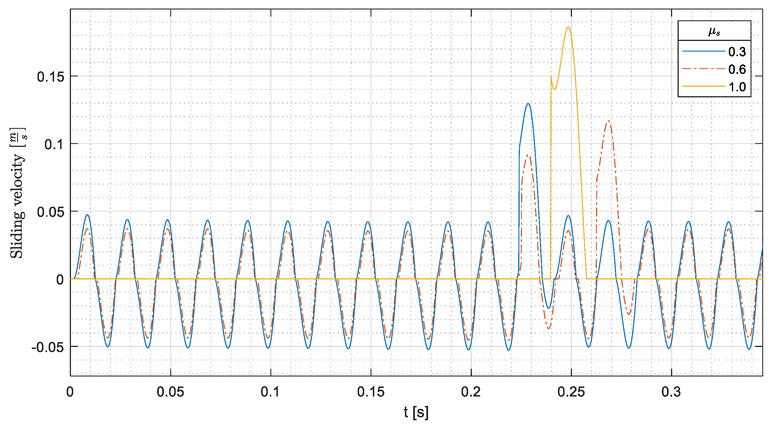
Figure 14 shows that ${\mu }_s$ has a small effect on phase 1: if the static friction coefficient increases above 0.6, the traveled distance increases. This phenomenon can be explained looking at Figure 15, which shows the sliding speed for the same values of ${\mu }_s$. With ${\mu }_s=1$ during phase 1, the cylinder does not slide at all, and the traveled distance increases, since the pure rolling motion dissipates less energy than the rolling with sliding motion. It is worth noticing that this result agrees with the analytical results of Figure 4.

After the first rebound, the impacts take place at random instants and, again, the relative velocity at the impact has the largest effect.

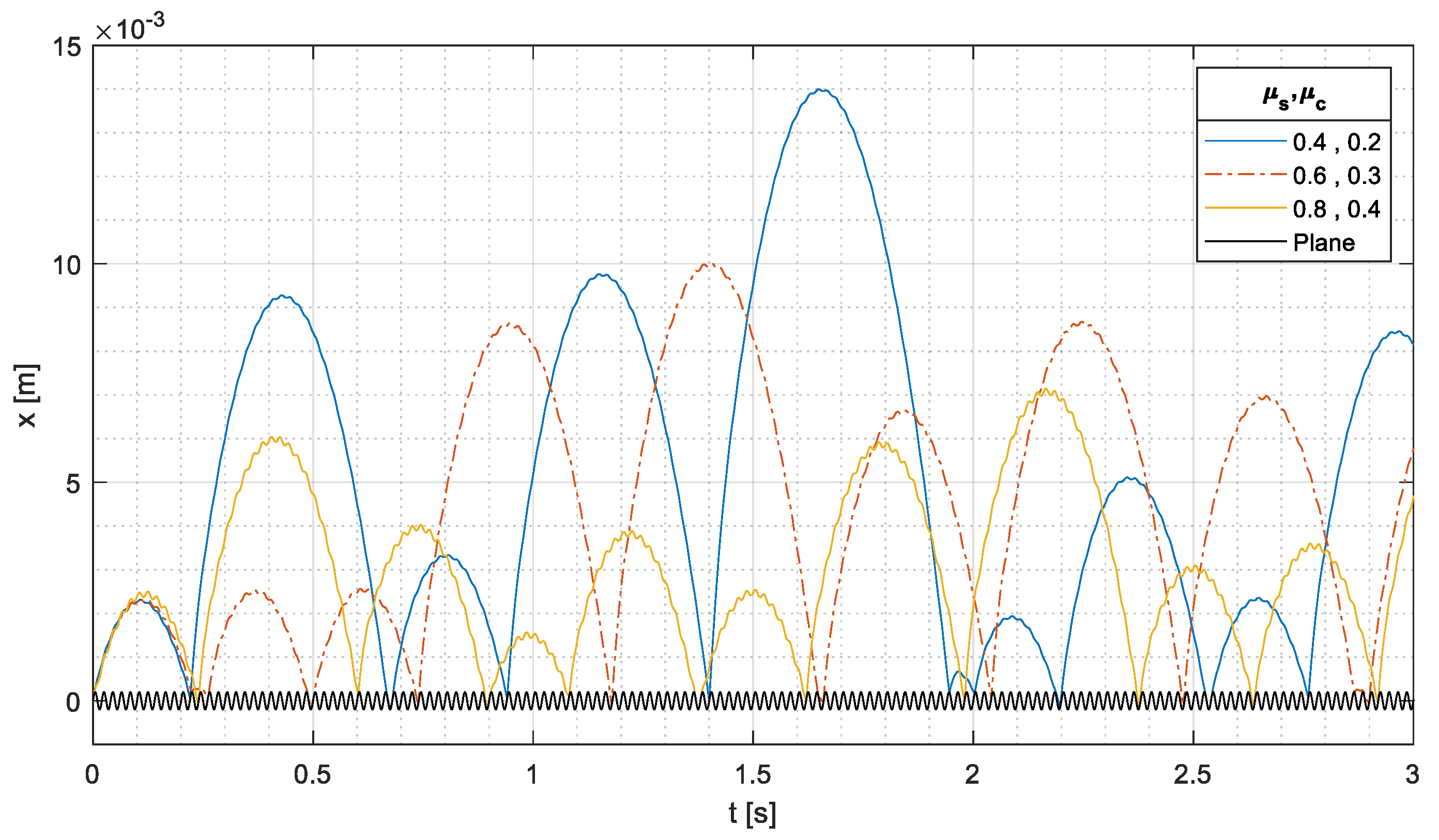
The effect of a proportional variation of both friction coefficients (${\mu }_c$ and ${\mu }_s$) is presented in Figure 16. In phase 1, the cylinder with the highest ${\mu }_s$ reaches the largest distance because it rolls without sliding, as shown in Figure 17. After the first impact (phase 2), the motion is dominated by the relative velocity at the impact; nevertheless, a decrease in ${\mu }_c$ leads to an average increase in the traveled distance. With ${\mu }_c=0.2$, there are 4 rebounds with a traveled distance larger than 0.008 m, whereas with ${\mu }_c=0.4$, there is no rebound with a traveled distance larger than 0.008 m. This phenomenon occurs because for every value of ${\mu }_c$ and ${\mu }_s$, there are large sliding velocities (Figure 17) after the impacts, and a reduction in ${\mu }_c$ leads to a reduction in energy dissipation.

The numerical results presented in this section clearly highlight that only the decrease in the vibration frequency can significantly increase the distance traveled by the cylindrical part. Nevertheless, even the largest traveled distances foreseen by simulations (0.043 m), which corresponds to about six times the cylinder radius, is not enough to cover the distances requested in many automatic manufacturing processes. For this reason, the development of a saw-teeth grooved surface of the conveyor track is highly recommended (see Figure 18). In this case, a traveled distance equal to 5 ÷ 6 times the cylinder radius is enough to move the cylindrical part from one grove to the following grove and to generate a sequential motion.

5. Comparison between Numerical and Experimental Results

In order to validate the numerical model, some experimental tests were carried out at the Laboratory of Robotics and Mechatronics of Padova University, which is equipped with the linear vibratory conveyor shown in Figure 19.

A track (120 mm long) with a stop plate was printed with additive manufacturing and mounted on the conveyor. A single steel cylinder was placed on the track. The motion was monitored by an AVT Pike f-032b camera with a frame-rate of 470 frames/s. Both the track and the cylinder were equipped with markers that were used to reconstruct their trajectories, using the Hough transform [20]. The static friction coefficient of the cylinder on the track was measured as well, and resulted in ${\mu }_s$= 0.7.

Figure 20 makes a comparison between numerical and experimental results. The numerical model is able to capture the most important features of cylinder motion, since the experimental results show a sequence of chaotic rebounds of the cylinder on the stop plate. The largest rebounds predicted by the numerical model have about the same duration (0.5 s) of experimental rebounds, and the traveled distances are only a bit larger (≈10%) than the measured values. This phenomenon may occur because, owing to the three-dimensional geometry of the system, the cylinder velocity may have a small component in the transverse direction ($z$ in Figure 18).

The main difference between numerical and experimental results is that the numerical model predicts a smaller number of bad impacts, with a short rebound. This happens because the numerical model is two-dimensional and assumes an impact between the cylinder and the stop plate along a line. In reality, the system is three-dimensional, and often the contact begins when a corner of the cylinder impacts the stop plate. The energy transfer from the conveyor to the cylinder is less efficient and leads to a reduced traveled distance.

These phenomena could be analyzed by means of a 3D numerical model, which would be much more complex and cumbersome than the presented 2D model (a 2D simulation lasting 1 s requires a computation time of about 16 s). Nevertheless, it is worth noticing that a complete agreement between numerical and experimental results could be difficult to achieve even with a 3D simulation, since the system is non-linear and chaotic; thus, small differences between simulation and experimental parameters may lead to large differences in results [19,21]. In actual conveyors, there are many cylindrical parts, and their collisions further enhance the chaotic behavior of the system [22].

6. Conclusions

The dynamics of vibratory conveying of cylindrical parts are very different from the dynamics of conveying of block-shaped parts. Both analytical and numerical calculations showed that large distances cannot be traveled owing to the backwards rotation of the cylindrical part.

The impacts of the cylindrical part on the stop plate are an essential feature of this kind of motion and strongly increase the traveled distance. After some rebounds, the impacts of the cylindrical part on the stop plate of the vibratory conveyor take place at random instants, which correspond to random values of the relative velocity between the cylindrical part and the stop plate. The impacts with the largest relative velocity lead to the largest rebounds. Eventually, the motion becomes chaotic.

Numerical simulations made it possible to investigate the effect of the most important parameters on the vibratory conveying of cylindrical parts. When vibration acceleration is kept constant, a decrease in vibration frequency leads to a relevant increase in the traveled distance. The kinetic friction coefficient (${\mu }_c$) influences the traveled distance; when ${\mu }_c$ halves, the maximum traveled distance almost doubles. The other parameters have a small or negligible effect on the conveying process. This phenomenon occurs because the energy transferred by the impacts to the cylindrical part essentially depends on the relative velocity between the part and the stop plate, and the variations in $\psi$, $f_v$, $k$ and ${\mu }_s$ have a small effect on the relative velocity but influence the instants in which the strongest impacts (with large relative velocity) take place.