Karst Spring Recharge Areas and Discharge Relationship by Oxygen-18 and Deuterium Isotopes Analyses: A Case Study in Southern Latium Region, Italy

Abstract

Karst aquifer recharge areas are usually difficult to identify because of the complexity of these aquifers’ characteristics. On the other hand, their identification is very important in the aim of protecting the groundwater resources that these aquifers host. Regarding this topic, this paper presents an approach aimed at identifying karst aquifer recharge areas by the application of oxygen-18 and deuterium isotopes composition of groundwater coupled with hydrological features. Oxygen-18 and deuterium isotope composition of Capodacqua di Spigno Spring, in the South of the Latium Region, has been applied with rainfall and discharge values related to the feeding aquifer of this spring. As δ¹⁸O and δ²H values of groundwater samples are natural tracers of the recharge area’s elevation, we propose a model, based on the distribution of the basin surfaces involved as recharge areas, in relation to elevations. The model estimates, for any discharge value, the percentage of the topographic area involved in the aquifer recharge. The setting up of this simulated distribution is supported by a Weibull cumulative probability function. The results show that the measured discharges increase as larger areas with lower elevations are involved in the recharge process.

1. Introduction

Well-developed karst aquifers, characterized by slow infiltration through the rock matrix and fast flow through conduits and fractures, represent highly productive groundwater systems with a high degree of heterogeneity and anisotropy. Therefore, identifying recharge areas coupled with karst aquifer hydrogeological characteristics, which are related to the main kind of groundwater drainage, is important information for sustainable management of these groundwater resources. This is important as groundwater coming from karst aquifers is a key source of fresh water for human supply [1].

In the study of karst aquifers, the employment of the environmental tracers can be considered as an effective method that allows an integrative investigation in order to perform adequate management of water resources [2]. Natural environmental stable isotopes together with other geochemical parameters are useful tools in cases where artificial tracing is not feasible such as at the scale of a regional aquifer system [3]. In particular, they have been applied to trace water flows inside the hydrological cycle from infiltration, influenced by chemical and isotopic precipitation characteristics, to discharge, due to water–rock interactions and geochemical processes [4,5]. In addition, radioactive isotopes like tritium (³H) provide information on groundwater circulation. This isotope is a useful tracer for determining the age of groundwater [6] and it has also been widely used to assess recharge and calculate the groundwater residence time [7].

The ¹⁸O and ²H data from groundwater are widely used to obtain information about the functioning of the karst systems [8], to determine important recharge areas of these aquifers, and to define the protection areas for the main springs [9]. The isotopic compositions of O and H in water, modified by meteoric processes are useful tracers for determining groundwater origin and movement because they generally do not change as a result of rock–water interactions at low temperatures [10]. Therefore, oxygen and hydrogen isotopes (δ¹⁸O and δ²H) can be used to determine the origin and path of groundwater and surface waters. In this regard, a similar systematic isotopic fractionation in stable hydrogen and oxygen occurs because their behaviour in the hydrologic cycle is similar [11]. This common behaviour leads to covariance between stable hydrogen and oxygen isotopic concentrations [11] defined by Craig [12] as the Global Meteoric Water Line (GMWL) relation. With the aim of determining groundwater recharge, residence times and water flow paths of oxygen-18 and deuterium have been extensively applied in catchment studies [13].

The present study focuses on qualitative-quantitative characterization of the karst aquifer feeding the Capodacqua di Spigno Spring, using isotopic tracers. In particular, oxygen-18 and deuterium isotopes have been applied, as environmental tracers of karst spring discharge, to determine the quantitative characteristics of Capodacqua di Spigno Spring. These stable isotopes, which have been already used in several studies to determine the mean altitude of the recharge area of aquifers [1,10,14], have also been involved in this study to define how the recharge area of Capodacqua di Spigno Spring varies according to the discharge, supplied by the same spring, in different periods of the year.

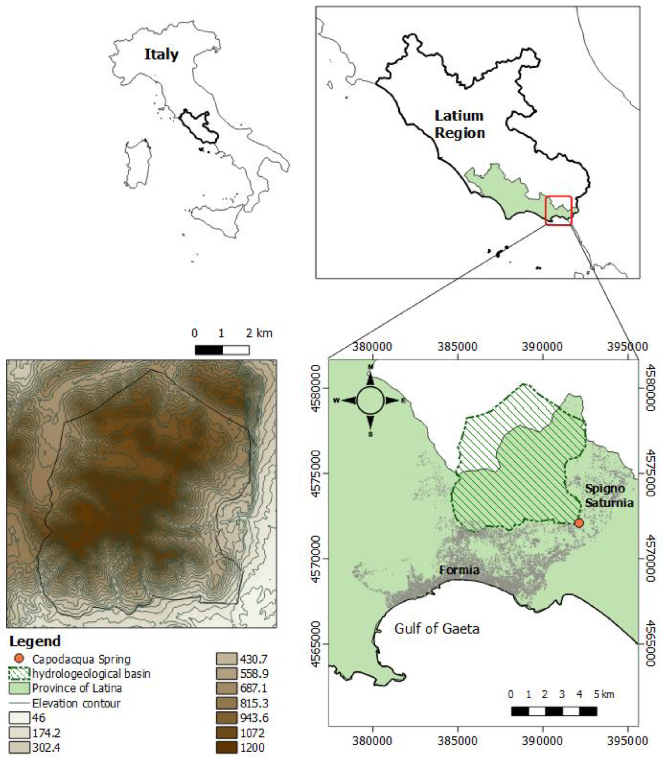
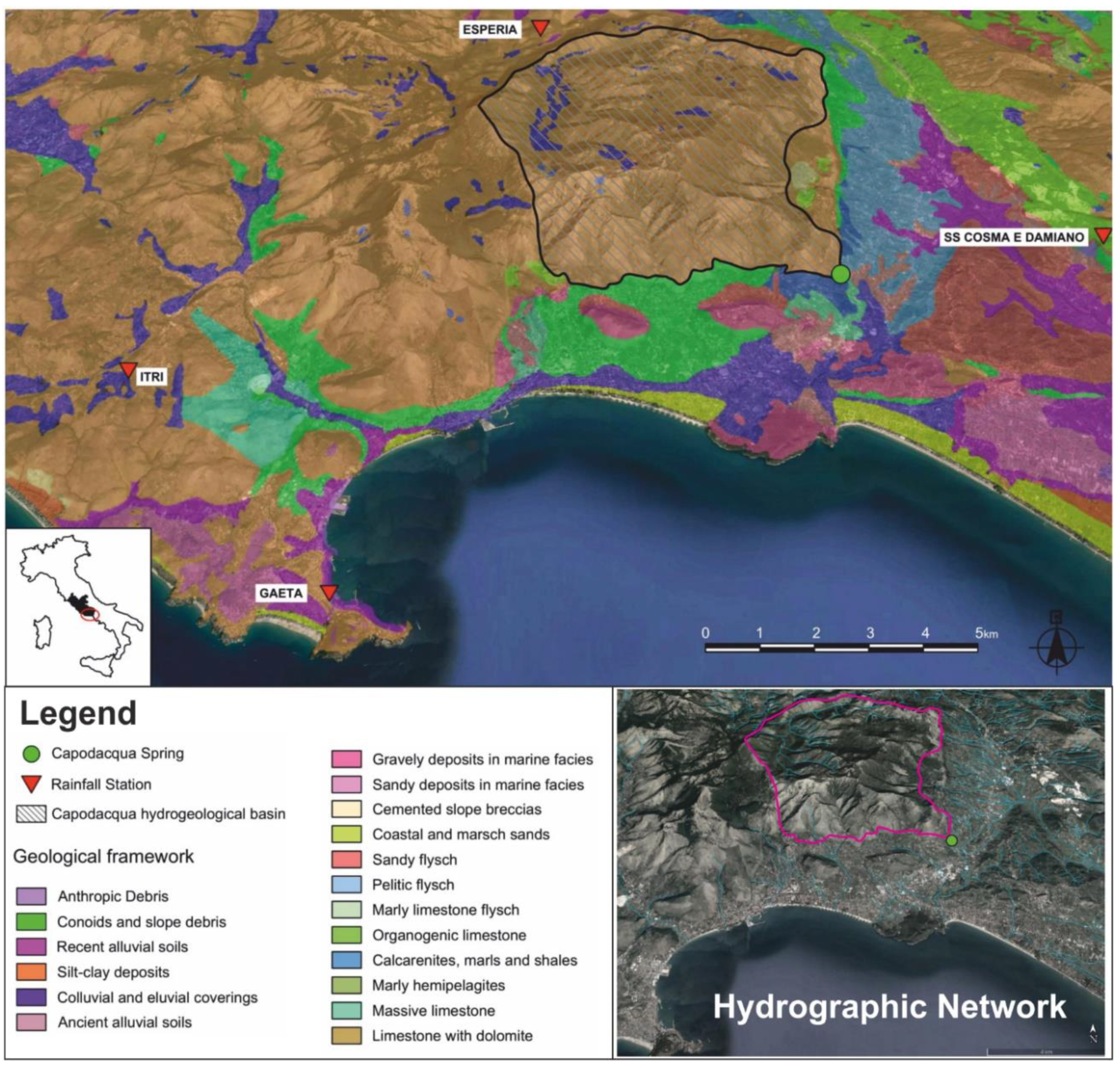
2. Geological and Hydrogeological Setting of the Study Area

Capodacqua di Spigno Spring, located in southern Latium Region (province of Latina), about 4 km from the Tyrrhenian Sea (Figure 1), is considered one of the most productive groundwater resources of Central Italy.

The study area is located in the karst coastal region of the Western Aurunci Mountains, which together with the Lepini and the Ausoni Mountains belong to the Pre-Apennines of Latium and form the carbonatic platform of the Volsci Ridge, separated from the Apennine ridge by the Latina Valley [15]. The hydrogeological basin of Capodacqua di Spigno Spring has a surface about of 51 km² and the spring is sited at an altitude of about 35 m a.s.l. The spring water comes out from the permeable limestone of La Civita Mountain and Castello Mountain and flows above the upper Miocene clays, at the lowest point of the limestone–clay contact [16].

Set over the fracture network induced by tectonic activity, the carbonate dissolution strongly influences groundwater flow and evolves into the limestone matrix.

The main karst landforms are rutted fields, karren, sinkholes, and swallow holes. The high permeability of karst features, together with the presence of karst depressions involves a rapid capture and infiltration of rainfall water into the aquifer. The karst depressions originated from the carbonate dissolution processes related to the contact between rainwater and carbonate rocks, which are part of the Capodacqua di Spigno Spring hydrogeological basin (Figure 2) [15].

The aquifer altitude ranges from about 100 m a.s.l. to about 1500 m a.s.l., with an average value of 880 m a.s.l; the limits of the aquifer are assumed considering the watershed topographic pattern. The altitude of the spring, instead, is of 35 m a.s.l.

The general groundwater flow direction in the aquifer is SE oriented, but there are also important local flows along the two faults that delimit the carbonatic series outcropping, especially that to the east, which seems to represent the main water conduit towards the spring [17].

3. Materials and Methods

Fourteen water samples, coming from Capodacqua di Spigno Spring, were analysed by the Isotope Geochemistry Laboratory of the University of Parma (Italy), using the IRMS (isotope-ratio mass spectrometry—Finnigan Delta Plus equipment) continuous flow-equilibration method with CO₂ for δ¹⁸O and H² for δ²H. Regarding the isotopic composition of rainfall water, no sampling was performed in the rainfall gauge stations considered in this study.

Isotopic abundance ratios are expressed as parts per million of their deviations, as given by the Vienna Standard Mean Ocean Water (VSMOW) Equation (1):

$$\mathsf{\delta }=\frac{\left({\mathrm{R}}_{\mathrm{sample}}-{\mathrm{R}}_{\mathrm{SMOW}}\right)}{{\mathrm{R}}_{\mathrm{SMOW}}}\times {10}^3$$

(1)

where R = ²H/¹H for hydrogen and ¹⁸O/¹⁶O for oxygen, the ratio of the heavy to light isotope and R_SMOW is the isotopic ratio of the standard (Standard Mean Ocean Water) [1].

Results, shown in

Table 1. Isotope composition of spring water samples collected from May 2018 to June 2019.

Date	δ18O (‰ VSMOW)	δ2H (‰ VSMOW)
26 April 2018	−7.2	−40.1
25 May 2018	−7.2	−40.4
27 June 2018	−7.3	−41.0
30 July 2018	−7.3	−41.1
29 August 2018	−7.3	−40.9
01 October 2018	−7.4	−41.2
08 November 2018	−6.9	−37.9
18 December 2018	−6.8	−37.6
18 January 2019	−7.1	−39.8
19 February 2019	−7.2	−40.3
20 March 2019	−7.3	−40.6
30 April 2019	−7.2	−40.1
29 May 2019	−6.7	−37.2
26 June 2019	−7.4	−41.2

, are expressed as per million deviations from the internationally accepted standard VSMOW according to Equation (1). The analytical error is ±0.2‰ for δ¹⁸O and ±1‰ for δ²H.

During the same days, that groundwater samples were taken, and discharge measurements were carried out along the river near Capodacqua di Spigno Spring, by the current-meter. The main equipment applied to measure the stream flow velocity is a SEBA horizontal axis current-meter F1. The SEBA current-meter has been used according to EN ISO 748:2007 requirements. This activity consisted mainly of measuring the excess flow rate of the spring in a discharge channel. In order to measure water velocity, we used the “Three-Point Method” described by the National Environmental Monitoring Standards (NEMS) [18]. Velocities were measured at 0.2, 0.6, and 0.8 of the depth below the surface.

Knowing the flow rate exploited by the local water management company, it was therefore possible to reconstruct discharge supplied by Capodacqua di Spigno Spring (

Table 2. Flow rates exploited for the local water supply (Qe), flow rate in excess measured in the river (Qm) and reconstruction of the discharges supplied by Capodacqua di Spigno Spring (Qs).

Date	Qe (l/s)	Qm (l/s)	Qs (l/s)
26 April 2018	519.57	915.00	1434.57
25 May 2018	505.80	780.00	1285.80
27 June 2018	537.00	490.00	1027.00
30 July 2018	542.85	250.77	793.62
29 August 2018	554.20	159.00	713.20
01 October 2018	489.02	168.42	657.44
08 November 2018	454.17	1656.66	2110.83
18 December 2018	486.26	2163.50	2649.76
18 January 2019	503.40	829.41	1332.81
19 February 2019	504.40	1050.16	1554.56
20 March 2019	454.39	836.56	1290.95
30 April 2019	433.16	558.05	991.20
29 May 2019	434.93	2500.00	2934.93
26 June 2019	458.03	671.46	1129.48

).

In this regard, Figure 3 shows the graph that compares the trend of monthly rainfalls, the exploited flow rates (in grey) and the delivered flow rates by the spring (in blue), calculated as the addition of the outflowing discharges, measured in the river section, and flow rates exploited by the local water supply agency.

4. Results

Groundwater samples have δ¹⁸O, as reported in Table 2, contents between a minimum of −6.74‰ with respect to VSMOW (29 May 2019) and a maximum of −7.37‰ with respect to VSMOW (01 October 2018 and 26 June 2019).

The isotope concentration values were plotted (Figure 4) together with the Global Meteoric Water Line (GMWL), the Mediterranean meteoric Water Line (MMWL) and two local meteoric water lines for central Italy, i.e., the two Central Italy Meteoric Water Lines (CIMWL), as proposed by Longinelli A. and Selmo E. [19] and Giustini F., Brilli M. et al. [20].

Figure 4 shows two regression lines, having different slopes. Besides the main trend line, whose slope is parallel to meteoric lines, there is one with a lesser slope that is relative to the waters sampled in the summer months. In this regard, the evaporation process can affect the isotopic composition of precipitation, atmospheric moisture and surface waters Evaporation of rainfalls results in the enrichment of the heavy isotopic species along the so-called evaporation line; it usually has a slope of less than 8 in δ(D) vs. δ(18O) space. According to this effect in this specific study case, Figure 4 shows higher δ-values for summer months’ samples. These enriched rainfall waters, due to a possible evaporation of rainwater, transfer their isotopic signature to groundwater at the moment of infiltration. Anyway, the hypothesis of re-evaporated effect on the precipitation and therefore on the contribution to spring discharge, can be validated by the knowledge of the rainfall water isotopic composition [14]. However, the main trend common to all values (Figure 4) depends on the variation of the infiltration altitude. On this base, the hydrological applications of stable isotope measurements are strictly related to an accurate knowledge of the vertical isotopic gradients that are generally used to calculate the mean elevation of the recharge area of aquifers. Air masses, rising at progressively higher elevations, expand adiabatically; subsequently, fractional condensation of water vapor takes place at decreasing temperatures from a water vapor that is progressively depleted in heavy molecules. This composite effect causes isotopically lighter precipitations with increasing elevations and is generally referred to as the “vertical isotopic gradient” [19]. Groundwater samples collected in 29 May 2019 and in 18 December 2018, regarding the events of maximum precipitation, show the similar highest content in heavy isotopes, despite the different rainfall regime, that characterized these two events. Therefore, this effect can be mainly attributed to the infiltration of the precipitation at a lower elevation than the water collected in all the other samples. As for the seasonality effect on groundwater, the enrichment in both heavy isotopes of meteoric waters is irrelevant in the warm months. In fact, in warm months (Figure 4) spring waters show lesser δ-values than the others. This effect is not in accordance with the seasonal effect characterizing the rainfall water which is found by P. Bono et al. [21] in a coastal area about 100 km away from Capodacqua di Spigno Spring. The effect of variation in isotopic concentration of the rainfall water is lesser on the isotopic concentration of the spring water than the altitude effect (Figure 4). This condition is probably due to the fact that spring waters are the result of several rain events occurring in different periods. Considering the natural attitude of the isotopic signature in depending on the infiltration altitude, groundwater sources may be studied using isotopes, e.g., ²H and ¹⁸O. Lower infiltration altitude will have precipitation characterized by an enrichment of heavy isotopes (²H and ¹⁸O) and vice versa. In this way, recharge zones are distributed depending on an altitude effect changing the isotopic composition of the water that feeds the spring [22]. The average values of vertical isotopic gradient, measured in Italy of about −0.24‰/100 m elevation for δ¹⁸O and −1.8‰/100 m elevation for δ²H, have been used [20]. In this regard, the local meteoric water line for central Italy defined in 2016 by Giustini F. et al. [20] is shown below:

$$\mathsf{\delta }\mathrm{D}=7.46\left(\pm 0.32\right){\mathsf{\delta }}^{18}\mathrm{O}+8.29\left(\pm 2.33\right)$$

(2)

According to this general behavioural trend, the spring discharge values, measured during the same days of groundwater sampling, have been compared with the average recharge area elevations values obtained using oxygen-18 and deuterium isotopes (Figure 5). It is evident that the measured flow rate increases when the average recharge area elevation values decrease by including lower elevations.

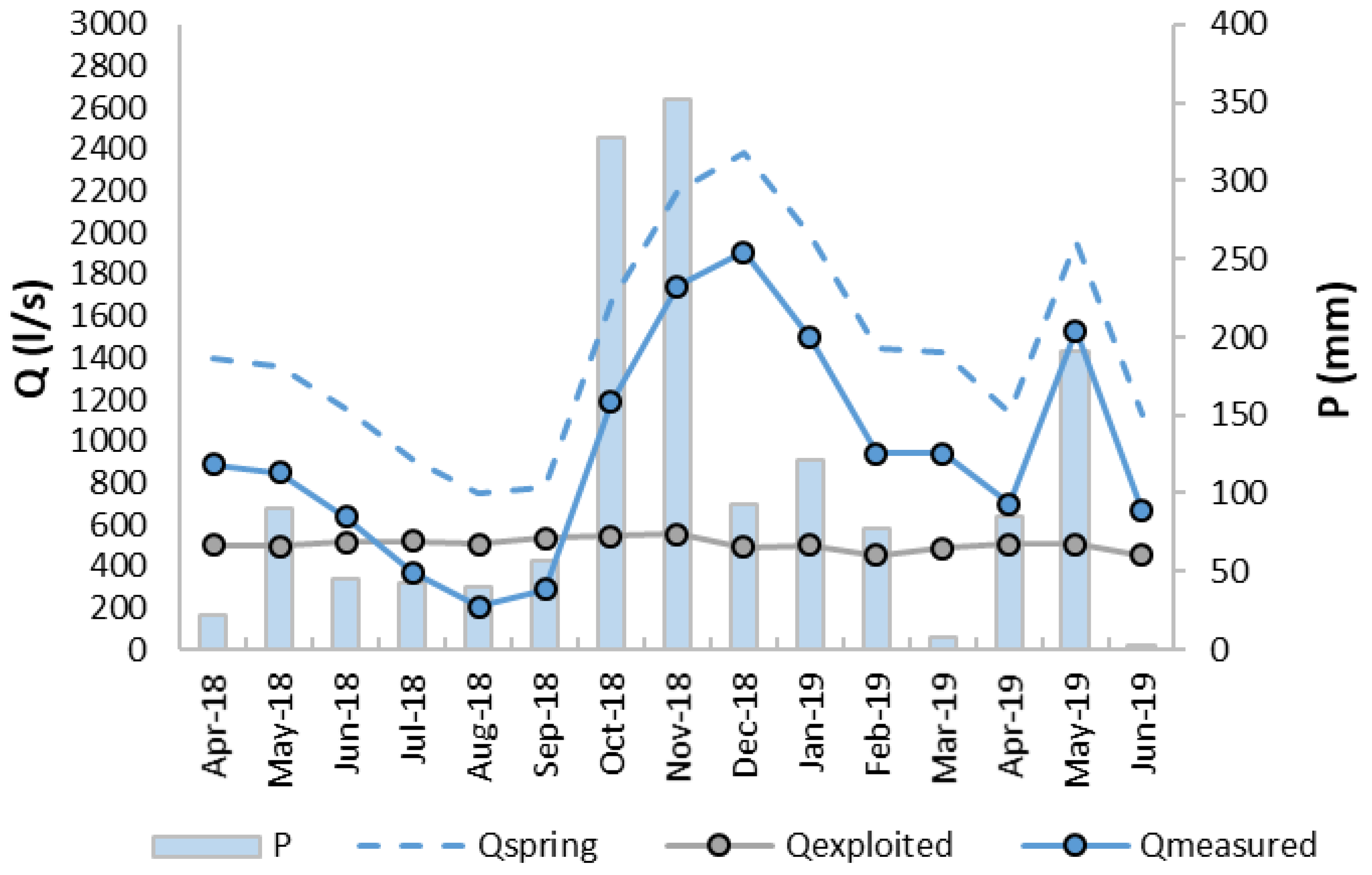
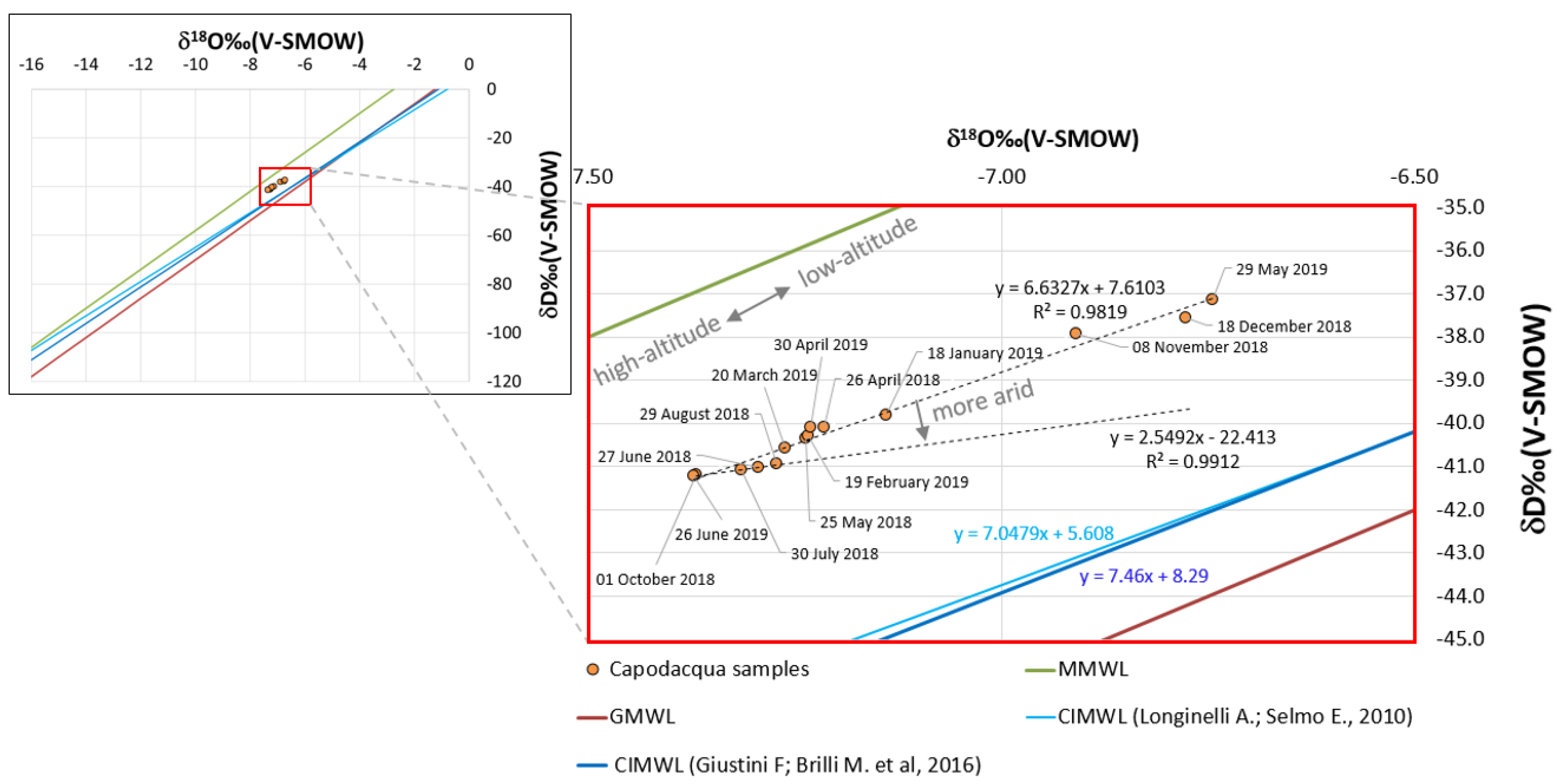
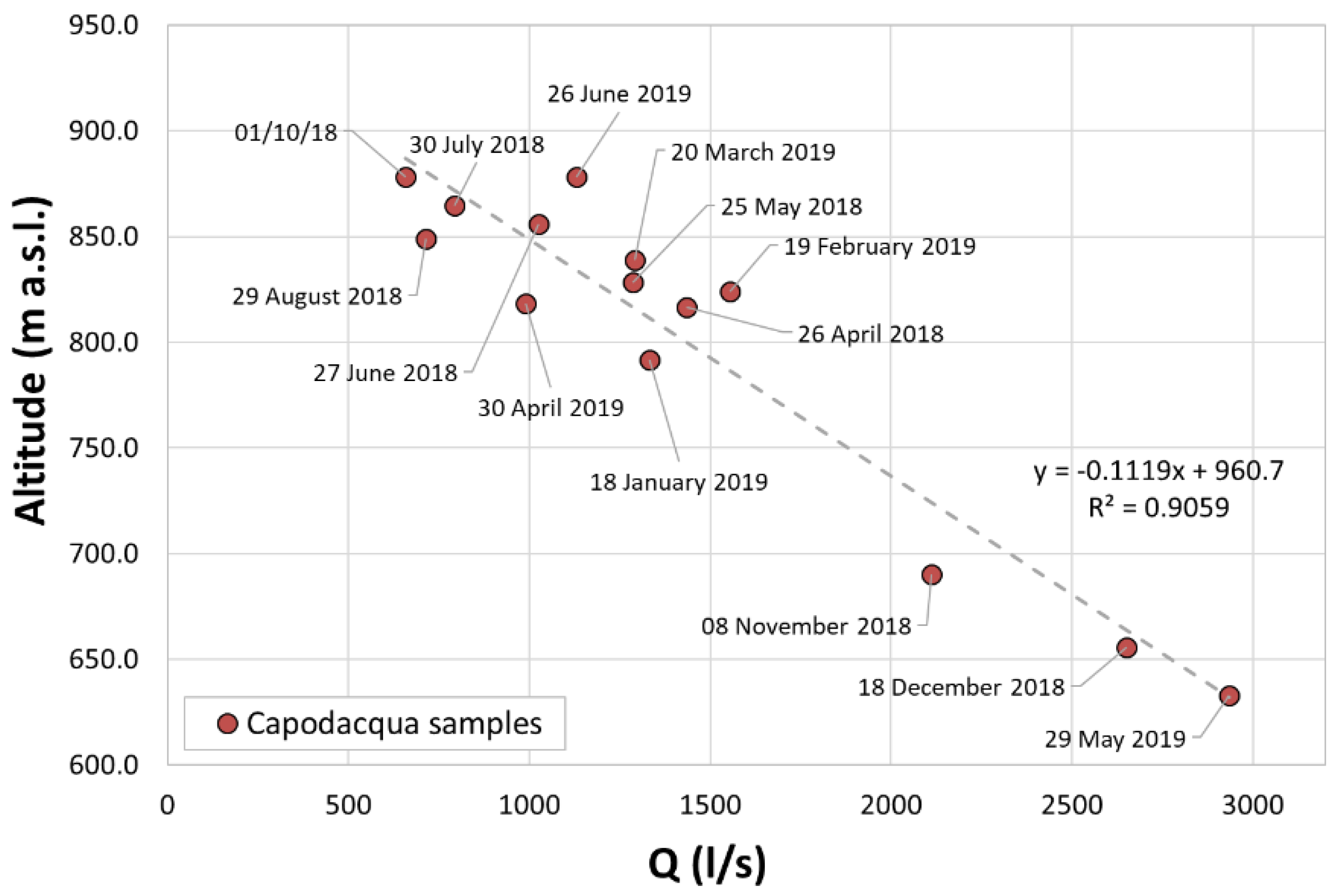
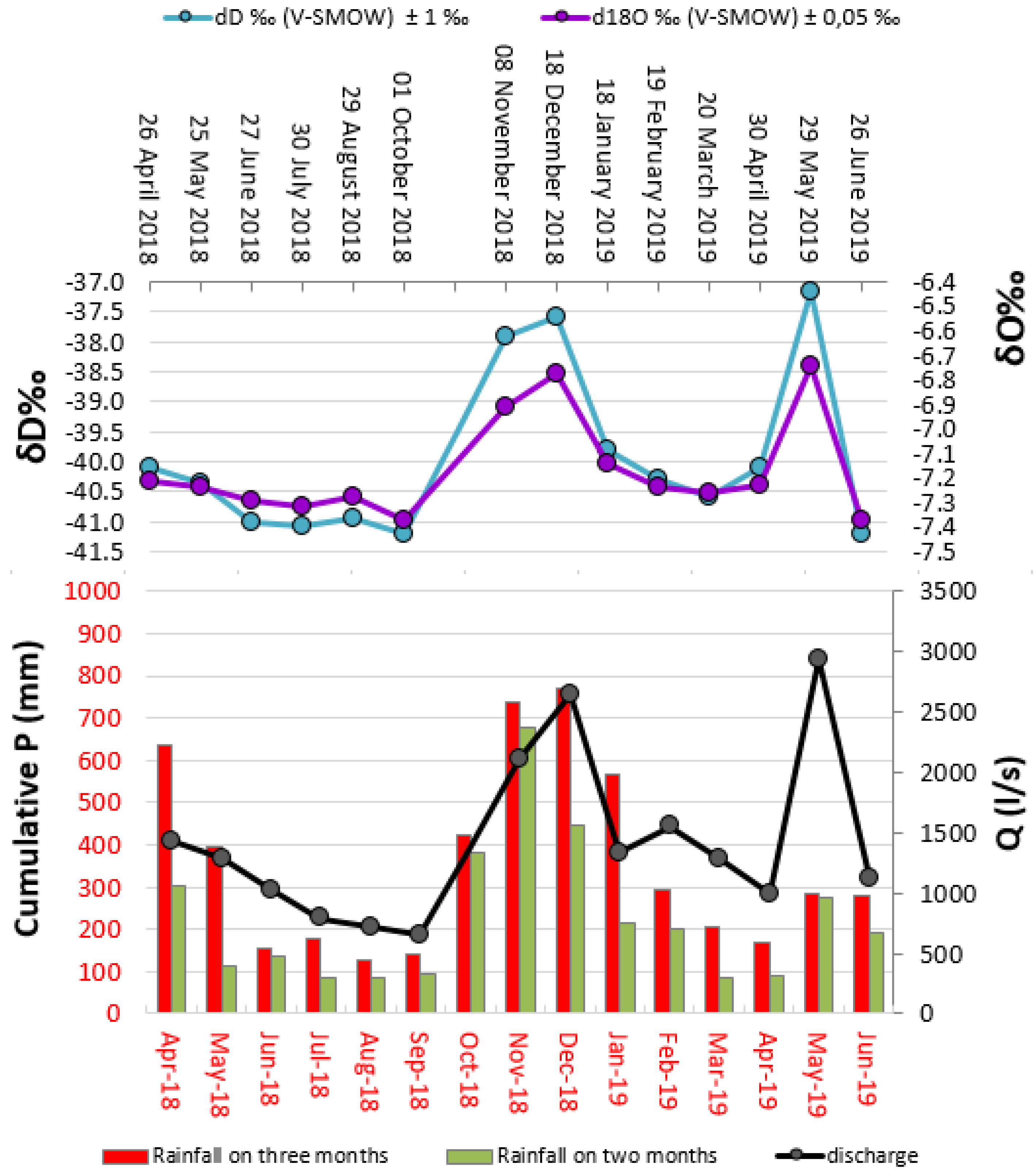
4.1. Spring Discharge Evaluation Using Oxygen-18 and Deuterium Isotopes as Natural Tracer

Spring discharge values were then compared with those of the stable isotopes, as reported in Figure 6. As the measured flow rate increases, enrichment in heavy isotopes also increases, both as regards oxygen and hydrogen. Previous studies about the relationship between spring discharge and isotopic rate show that this relationship can be connected to groundwater circulation features and, therefore, to their response to the rainfall intensity [23].

Figure 6 shows that the trend of the δ²H and δ¹⁸O values is comparable to that of the discharge delivered by Capodacqua di Spigno Spring. Specifically, the correlation between spring discharge and δ²H‰ and δ¹⁸O‰ values has a R² parameter of 0.903 and 0.900, respectively. However, it can be noted that there are some inconsistencies; for example, the waters sampled on 01 October 2018 and 26 June 2019 have identical δ²H and δ¹⁸O values, but, in the two days, two different flow rates were measured. The discharge supplied by the spring on 01 October 2018 is 657.44 l/s, while that delivered on 26 June 2019 is 1129.48 l/s, therefore they are substantially different. Another difference between the trend of stable isotope values and the flow rates trend concerns the data referring to 19 February 2019: the spring discharge value shows an increase compared to the previous month, the values of δ²H and δ¹⁸O, instead, show a decreasing trend. These incongruities can be explained by analysing the monthly rainfall analysis. Therefore, it is necessary to analyse also the influence of the monthly rainfall trend on the spring discharge. In particular, this effect is shown in Sappa et al. [15], where the Capodacqua di Spigno discharge is affected by rainfall values referred to as lag-time of five months with a maximum influence related to the 2nd and 3rd of previous months (Figure 6). The increase of the flow rate supplied by the spring in June was not detected by the isotopic values; this effect may probably be due to the relevant rainfall intensity occurring in the previous months. In addition, the discrepancy concerning the data of 19 February 2019 can be explained by the analysis of the monthly rainfall. In this case, we can see that the spring discharge trend reflects the monthly rainfall in general terms. In this way, the discharge regime that occurred in the wet period (October–January) is in accordance to the two and three previous cumulated rainfall months. With regard to the maximum discharge measured in May 2019, this event seems to be related to a daily event occurred close to the detection day. Therefore, this impulsive temporal discharge event mainly contains the rainfall infiltrate at low elevations, which is also detected by isotopic concentration yet, as shown in Figure 5. However, for the assessing of the spring response to the rainfall input, we need to consider other parameters that control the dynamics of the aquifer system. On the other hand, the aforesaid incongruities can be also due to the isotopic concentration variability of the rainfall water in the different periods of the year. This effect was discussed in many groundwater studies [24,25]; they suggest that a future study needs to take into account the rainfall isotopic composition. The rainfall water sampling will allow us to correct the input data, which are subsequently introduced in the proposed model. This one also for take into account the seasonal variation comprises from November (minimum) and May (maximum) highlighted in a study [21] regarding the rainfall water isotopic concentration detected in central Italy, near the study area.

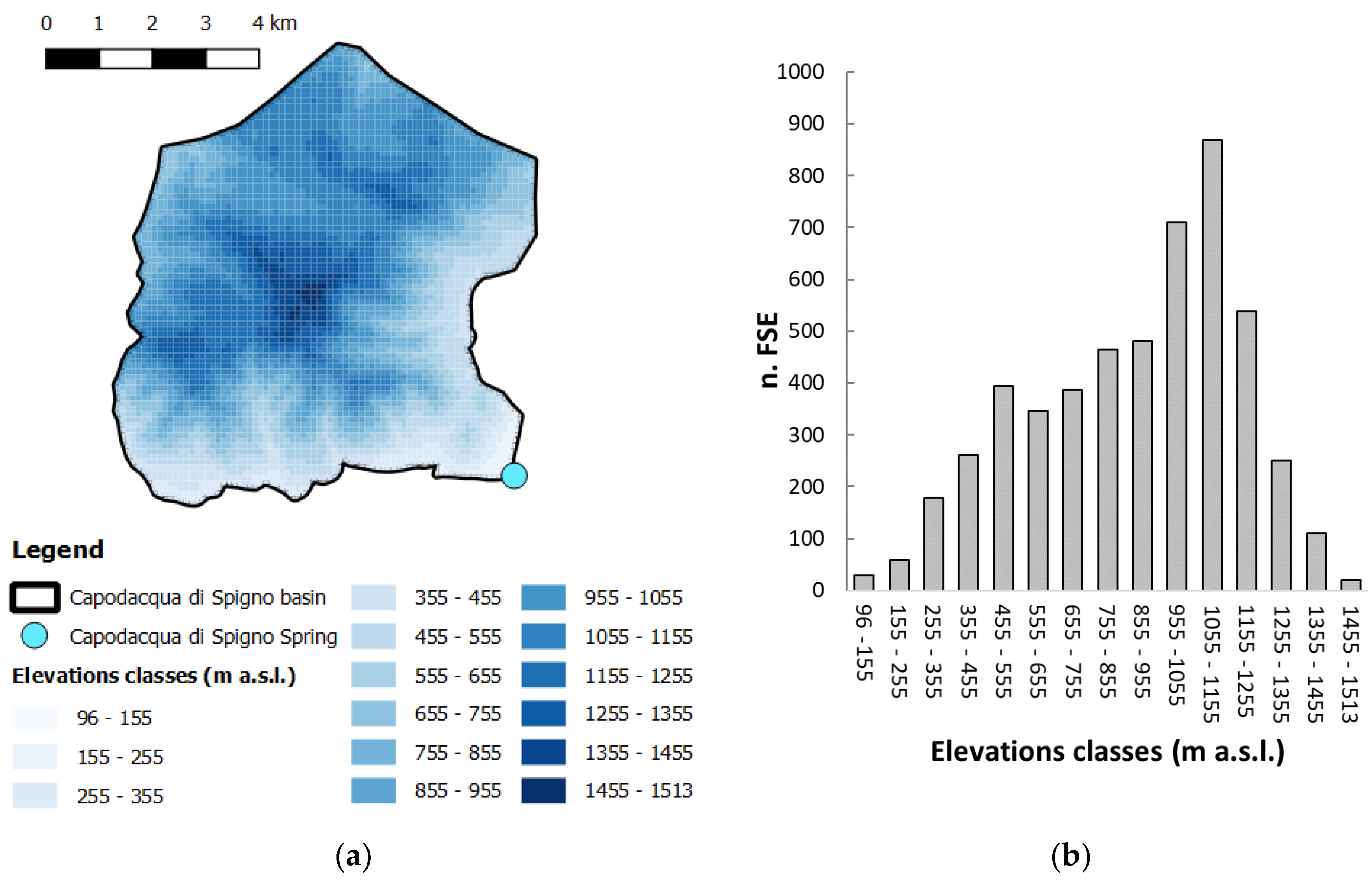
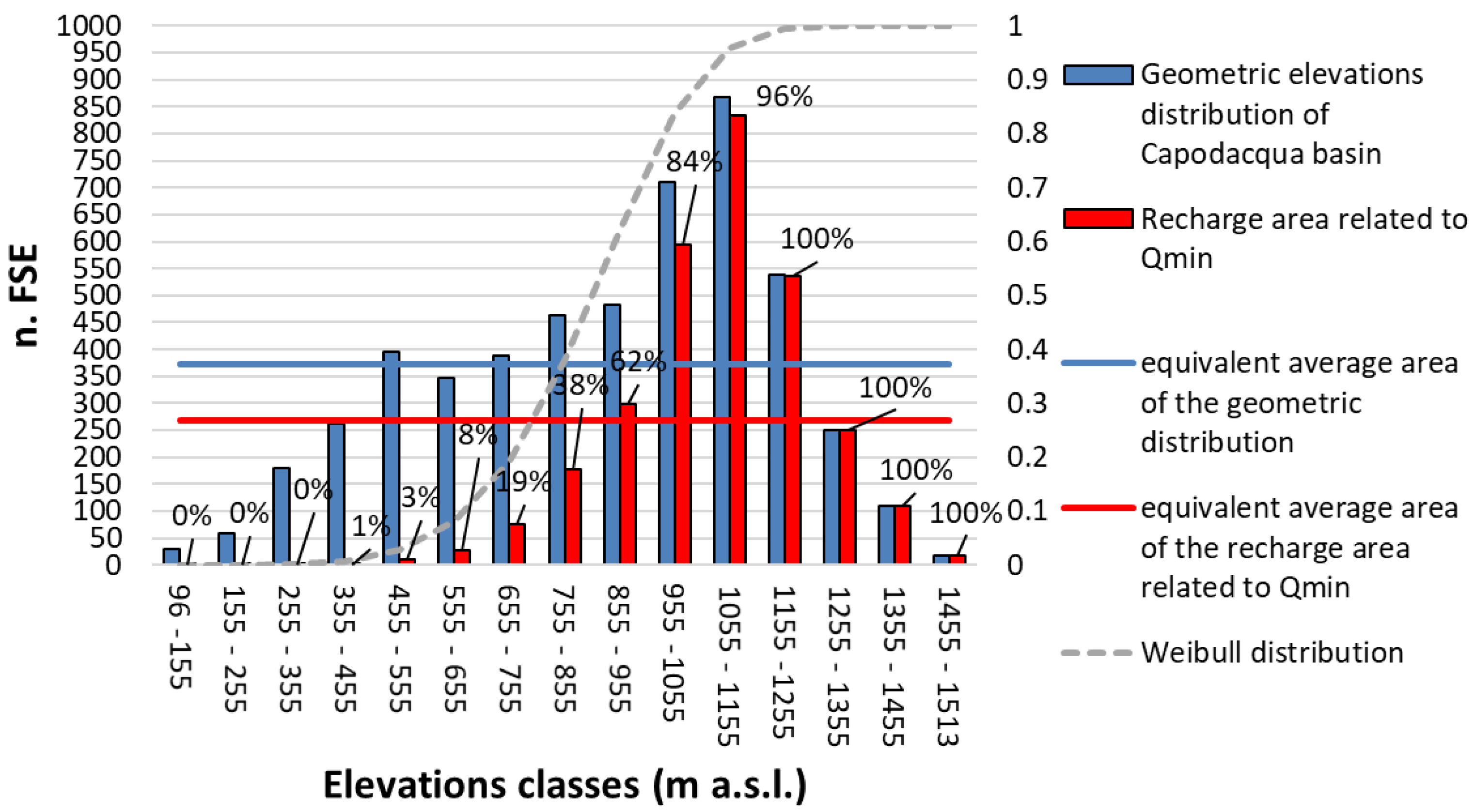
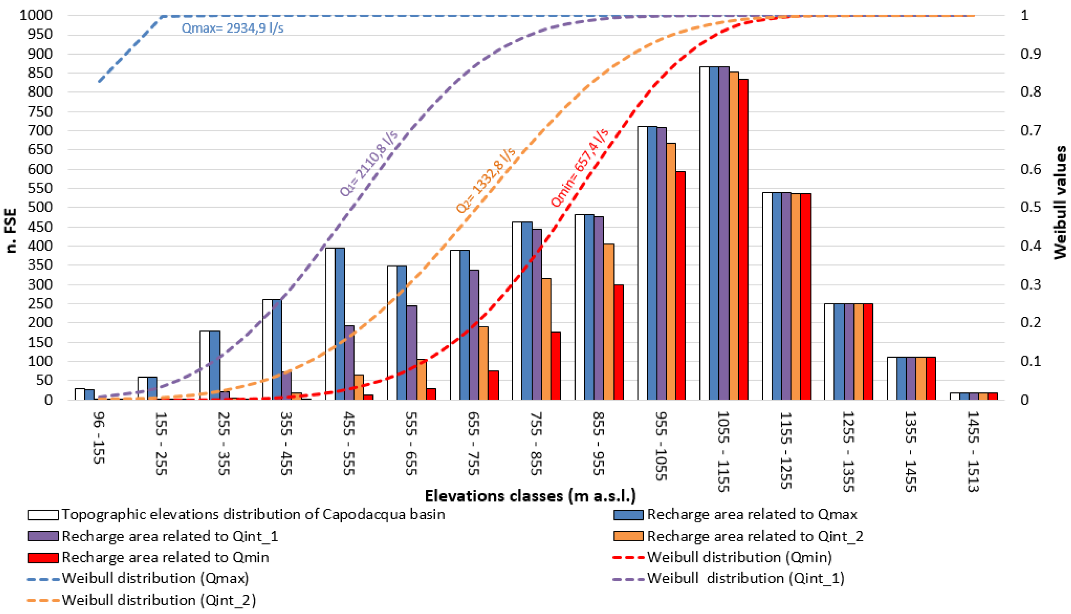
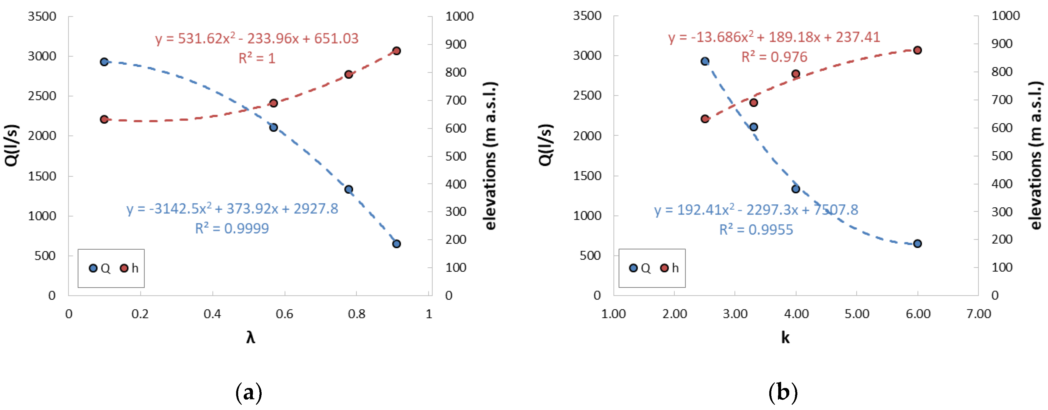
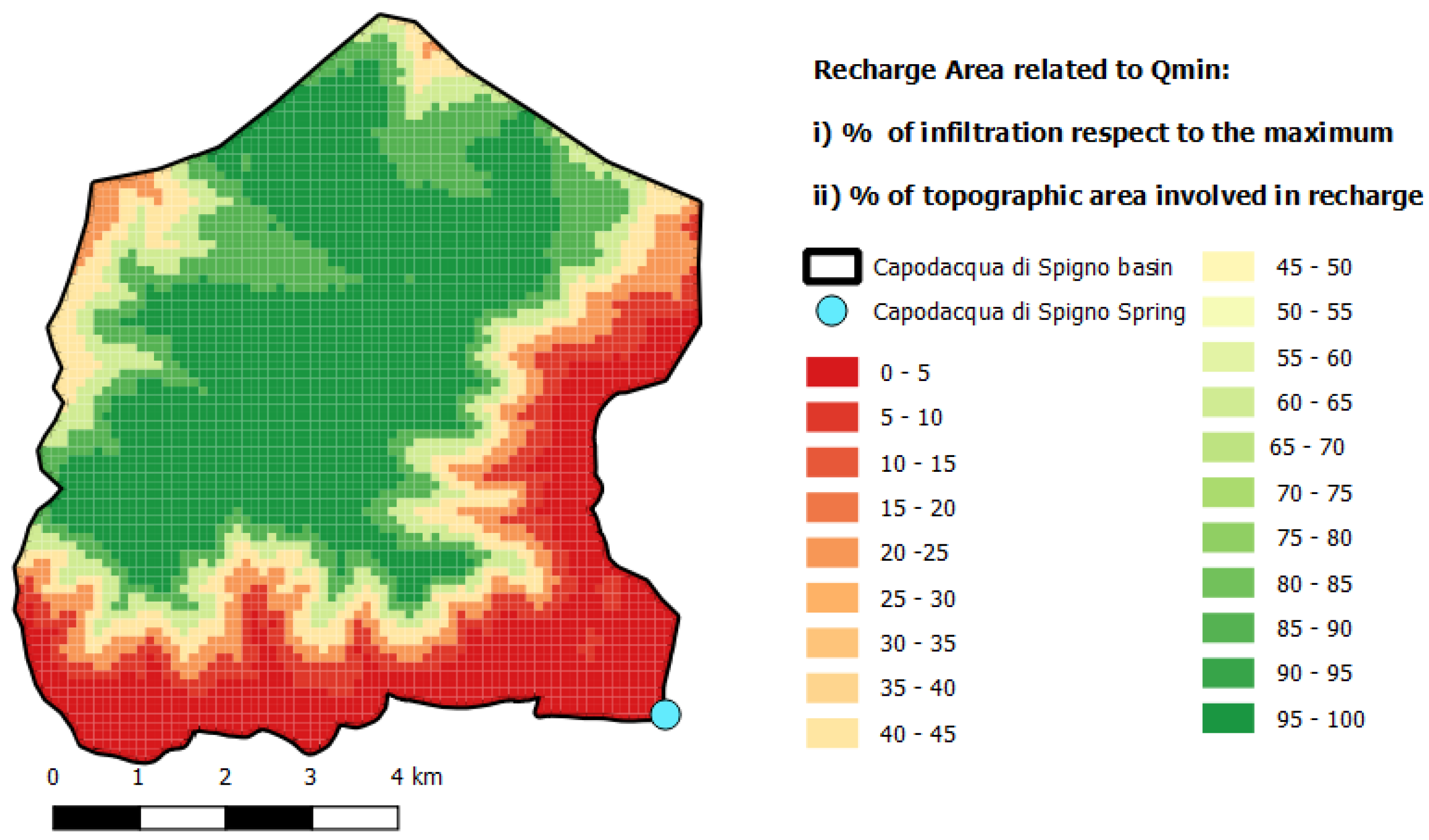
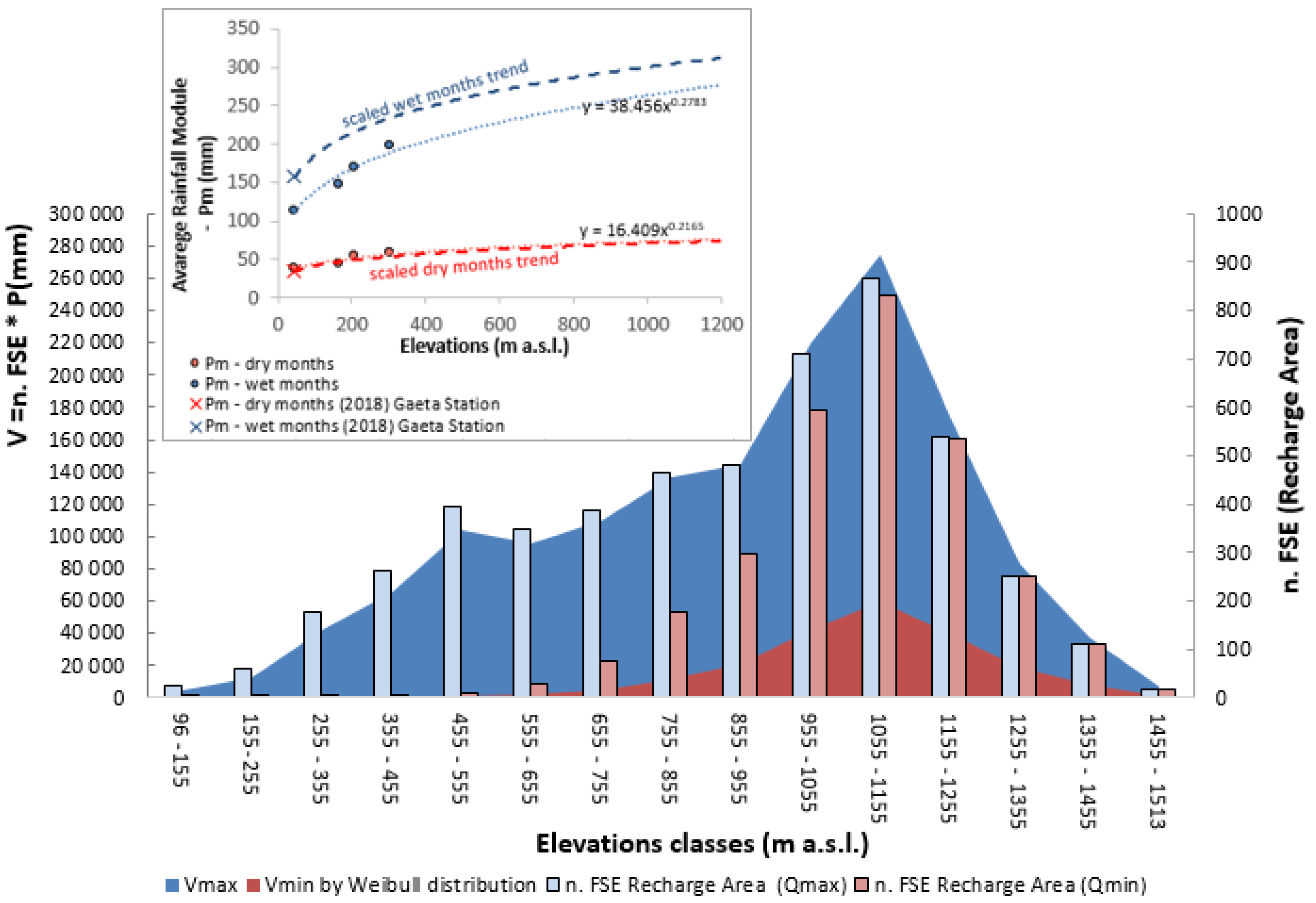
4.2. Spring Recharge Area Identification by Using Isotope-Driven Model

Starting from the digital elevation model (DEM) of the study area, the basin has been discretized into finite square elements (FSE) with the size of 100 × 100 m. Therefore, a unique elevation value has been attributed to each of the cells of the grid. In this way, it was possible to define the elevation classes distribution of the topographic surface of Capodacqua di Spigno Spring basin as represented in Figure 7, which shows that the topographic surface distribution of this basin is typical of a carbonate karst aquifer. In fact, the depression areas are due to karst landforms, such as dolines, karren, dry valleys, swallow holes and poljes. In this regard, the irregular elevation distribution of the area is mainly due to the presence of a karst-prone large depression area at higher altitudes. In particular, the most representative classes are around 950 and 1155 m a.s.l., while the classes at a lower altitude range (95–255 m a.s.l.) show a low-frequency distribution that is due to the presence of steep topographic slopes in that range. These slopes evolve towards more flat topography in the higher elevations. According to the aforementioned conceptual model, we propose, about the study area and similar areas, an analytical model aimed at identifying the main recharge areas according to the isotopic rates variation, detected in groundwater samples, taken at the spring. The model is a not time depending model, this one by using the relationship between the natural elevation distribution of the feeding basin and the isotopic rate distribution of groundwater samples, identifies the main recharge zones that contribute to the spring discharge. Regarding the distribution, the model defines the recharge areas considering two different output assignment conditions, in a non-combined way. These conditions are referred to as: (i) uniform rainfall distribution on the same elevations classes, on the topographic surface of the basin; (ii) rainfall events that involve specific and limited zones within the basin, both depending only on elevation. In addition, in the distribution of the recharge area with the elevation, the proposed model does not take into account the different soil permeability and runoff effects depending on the slope of the surface. However, these effects can be considered by an evolution of the proposed model regarding their influence on elevation classes. The proposed model is based on setting up a linear relationship between discharge values and δ²H and δ¹⁸O rates at the same time monitored at the spring (Figure 5). Therefore, concerning the discharge, it is possible to assume that the average elevation of the recharge area, obtained by using isotopic concentrations, can be referred to as a prevalent sector of the topographic surface of the basin that is depending on the elevation.

In this study case (Figure 5), the minimum discharge value of 657 l/s refers to the average recharge area altitude of 878 m a.s.l., while the maximum discharge of 2935 l/s refers to the average recharge area elevation of 633 m a.s.l. These values are defined as the average of the two average recharge area elevations, obtained using δ²H and δ¹⁸O concentration values. Considering the topographic distribution of the area in relation to the elevation, it is possible to associate a theoretical regular aquifer having the same equivalent area, A_eq, for each altitude. This area is computed in term of weighted average, on the elevation classes (n. 15 in this case), as follows:

$${\mathrm{A}}_{\mathrm{eq}}=\frac{{{\displaystyle \sum }}_1^{\mathrm{n}}({\mathrm{A}}_{\mathrm{i}}·{\mathrm{h}}_{\mathrm{i}})}{{{\displaystyle \sum }}_1^{\mathrm{n}}\left({\mathrm{h}}_{\mathrm{i}}\right)}$$

(3)

where A_i is the area related to ith-elevation hi.

In this model, we consider the maximum discharge of the time series, associated to the complete topographic elevation distribution of the area, as wholly involved in the recharge area. Therefore, considering Equation (3), it is possible to associate for this condition an equivalent average area which is distributed on all the altitudes, A_{eq_max} = 372.83 n. FSE having the same elevation, detected by isotopic rate referred to the maximum discharge. Considering, in addition, the linear relation showed in Figure 5, it is possible to assume that minimal spring discharge is associated with a smaller recharge equivalent area (A_{eq_min}), having a higher elevation detected by isotopic ratio values, by using the general following equation:

$${\mathrm{A}}_{\mathrm{eq}\_\mathrm{j}}=\frac{{\mathrm{A}}_{\mathrm{eq}\_\max }·{\mathrm{h}}_{\mathrm{q}\_\max }}{{\mathrm{h}}_{\mathrm{q}\_\mathrm{j}}}$$

(4)

where A_{eq_j} is the generic recharge area associated to the generic jth-discharge, which corresponds to an average elevation h_{q_j}, obtained by isotopic concentration values. In this way, it has been obtained that the equivalent minimal recharge area, A_{eq_min}, is of 268.79 n. FSE associated with the maximum average recharge area elevation of h_{q_min} of 878 m (Figure 8).

Having obtained the generic couple values of A_{eq_j} and h_q-j, for this average equivalent aquifer condition, the model provides a way to perform a simulated distribution of the recharge area on the geometrical elevations classes by considering conservative recharge areas at higher elevations. This condition matches the natural rainfall trend, which is typical of mountain aquifers. The simulated distribution, which is shown in Figure 8 for minimal spring discharge, is demanded by a Weibull cumulative probability function; this function is widely used to explain the distribution of natural events [26,27,28] because it can be associated with cumulative normal or non-normal distribution of many natural parameters. Specifically, we use the two-parameters Weibull function as follows:

$$\mathrm{F}{\left({\mathrm{h}}_{\mathrm{i}},{\mathrm{A}}_{\mathrm{i}},\mathrm{k},\mathsf{\lambda },\right)}_{\mathrm{i}}={\mathrm{A}}_{\mathrm{i}}\left(1-{\mathrm{e}}^{-{\left(\frac{{\mathrm{h}}_{\mathrm{i}}}{\mathsf{\lambda }}\right)}^{\mathrm{k}}}\right)$$

(5)

where h_i is the central value of the class elevation associated to the topographic ith-class area A_i, while k and λ are the shape modelling parameters of the function.

These shape parameters are found by iterative trial; specifically, the values change, in a limited range, up to the convergence of the following condition:

$${\mathrm{A}}_{\mathrm{eq}\_\mathrm{j}}={\mathrm{A}}_{\mathrm{eq}\_\mathrm{weibull}}\to \frac{{\mathrm{A}}_{\mathrm{eq}\_\max }·{\mathrm{h}}_{\mathrm{q}\_\max }}{{\mathrm{h}}_{\mathrm{q}\_\mathrm{j}}}=\frac{{{\displaystyle \sum }}_1^{\mathrm{n}}{\mathrm{A}}_{\mathrm{i}}\left(1-{\mathrm{e}}^{-{\left(\frac{{\mathrm{h}}_{\mathrm{i}}}{\mathsf{\lambda }}\right)}^{\mathrm{k}}}\right){\mathrm{h}}_{\mathrm{i}}}{{{\displaystyle \sum }}_1^{\mathrm{n}}\left({\mathrm{h}}_{\mathrm{i}}\right)}$$

(6)

where the $A_{eq\_weibull}$ is the weighted average area computed using the Weibull function. By resolving Equation (5) for other intermediate values of discharge and their isotopic concentration, Figure 9 shows that the model progressively involves lower elevations areas, at the same time as discharges increases. In particular, the recharge areas having elevations over 1155 m are always quasi-totally involved in any spring discharge values. In addition, out of the maximum discharge Q_max, it is possible to notice that the average elevation of the recharge area, detected by using isotopic concentrations, is in accordance with the upper “rollover” of the Weibull curves. This condition implies that the recharge area, relative to each spring discharge value and to each isotopic value obtained from the groundwater sample, is characterized by a fast decrease of areas with elevations lower than the average elevation of the recharge area detected by isotopic concentration. We have used intermediate discharge values, Q₁ (08 November 2018) and Q₂ (18 January 2019), in order to define also the model parameters relative to areas between the maximum and minimum recharge areas (Figure 5).

The shape of Weibull coefficients λ and k, found for the four conditions mentioned before (Q_max, Q₁, Q₂ and Q_min) and reported in

Table 3. Parameters used for the calibration of the model.

	Q (l/s)	h (m a.s.l.)	λ	k
Qmax	2934.9	633.0	0.10	2.50
Q1	2110.8	690.0	0.57	3.30
Q2	1332.8	791.5	0.78	4.00
Qmin	657.4	878.0	0.91	6.00

, show a good correlation with elevations and discharge values (Figure 10). With reference to the latter, Weibull coefficients show a good non-linear correlation. This condition permits us to use the two diagrams in Figure 10 as a tool to obtain the correlation between the discharge and average elevation by using the aforesaid coefficients as driver values and vice-versa. This correlation shows a good robustness that is reflected in the acceptable estimation of the discharge and of the recharge area average elevation, for all other values of the data-set (Figure 5). In this way, the use of both plots (Figure 10) allows us to obtain also the two shape coefficients used in Equation (5) to estimate the topographic area involved in the recharge area that supplies the spring discharge.

Through knowledge of the recharge areas depending on elevation, it is possible to perform a map of the simulated distribution of these areas. Referring to the model setup, the map (Figure 11) can take into consideration the two different model conditions, one at a time. In particular, (i) different rainfall infiltration rate uniformly distributed with elevation; (ii) local storm events that involve limited zones within the elevations range (elevations classes). In this way, concerning the spring discharge minimum value, Figure 11 shows the map of the simulated distribution of the percentage of topographic elevation classes, in terms of area, involved in recharge, or, with a different interpretation, the map of the simulated distribution of the percentage of infiltration with respect to the maximum. Both the interpretations obtained coming from the application of the same Weibull cumulative distribution obtained by Equation (5). This map shows that for the spring discharge minimum value a large part of the area at the base of mountain aquifer (red area) is weakly or not engaged in recharging. By contrast, the area belonging to the mountain plateau upper 1100 m (green area) is totally engaged in the aquifer recharge.

The simulated distribution of recharge areas, defined by the model, can be also related to the variability of rainfall intensity that involves the basin, too. Specifically, this variability takes into consideration the natural trend of the rainfall intensity increasing with elevation. In particular, for the rainfall–altitude relationships, we use the exponential relationships to obtain much more plausible values in the case of mountain basins [29]. This last relationship was used with the aim to quantify the infiltration volumes related to the maximum and minimum spring discharge (Figure 12). In particular, the rainfall–altitude relationships associated to maximum and minimum discharge were respectively assumed to refer to the average of the four wet months (October–January) and the four dry months (June–September), computed considering the historical data-set (40 years: 1959–1999). The thermo-pluviometric stations taken into consideration are Gaeta (45 m a.s.l.), Itri (165 m a.s.l.), Esperia (302 m a.s.l.) and SS Cosma e Damiano (206 m a.s.l.) (see you Figure 2). The regression laws relating to the aforementioned wet and dry period in the time frame of the case study (April 2018–June 2019) were recomputed. This operation was performed by scaling the rainfall values, up to the target Gaeta station values, measured in this time frame. This recomputing operation was necessary because only the data coming from Gaeta thermo-pluviometric station were available in 2019. Therefore, considering the real involved recharging areas driven by the isotopic signature, it was also possible to perform the assessment of the rainfall water volumes. The rainfall volumes regarding the two aforesaid rainfall regimes related to maximum and minimum discharge values. The relative volumes, V_max and V_min, result from the product of the recharge area and the rainfall values, which were both taken into relation with elevation classes (Figure 12). Taking into account the effects of evapotranspiration, the maximum infiltration volumes were reduced by about 60%; at the same time, the minimum infiltration volumes tend to zero due to the high temperatures encountered in summer. These conditions lead to the identification of the minimum flow rate not directly connected to the rainfall that fell during the dry months, but somewhat dependent on the greater rainfall that fell at high altitudes in the previous months, mainly intercepted by the greater area available at those altitudes and, subsequently, arrives later at the spring output; as it commonly occurs in the regional karst aquifers [30]. This effect is in accordance with the isotopic signature that marks higher elevations at minimum discharge.

5. Discussion

Generally, ¹⁸O and ²H isotopes are used only to identify the main recharge areas of aquifers. However, in this study case, the contemporary measurement of the spring discharge and the concentrations of the aforementioned stable isotopes permitted us to obtain a good correlation between these parameters. Therefore, ¹⁸O and ²H isotopes can be good natural tracers of the flow rate supplied by the spring, also without taking into account the rainfall regime that is the main factor influencing the spring discharge. Nevertheless, in this paper, we argue for the possibility to use the δ²H and δ¹⁸O isotopic values as tracers for identifying the main recharge areas related to different discharge values detected in the spring, during the hydrological year. Specifically, we introduce a model able to identify the percentage of the topographic area-elevation classes involved in recharge. This model defines the recharge areas considering two different output assignment conditions, both in a non-combined way. These conditions are referred to as: (i) uniform rainfall distribution on the topographic surface of the basin; (ii) rainfall events that involve specific and limited zones within the basin, both depending only on elevation. Besides, in consideration of the nature of the phenomenon that influences the concentration of isotope values, the model is non-dependent on the delay time between infiltration and spring flow rate. In addition, the model defines the recharge areas but not the temporal distribution of the rainfall events that determined the isotopic concentration measured in the spring. In this regard, the isotopic groundwater signature suggests that the lower spring discharge values are related to the rainfall water infiltrated at previous period and at the highest altitude (higher distance from the spring). Despite the aforesaid limitations, the proposed model correlates the spatial distribution of the recharge area (infiltration area) with the spring discharge.

In general, the model is based only on the isotopic concentration measured in the spring. Theoretically, this concentration remains constant if the rainfall intensity increases and the recharge area remains the same. On these bases, the fact that the isotopic concentration increases with discharge values admits that the discharge increases with an increase of the recharge area (isotopic ratio dependent) in relation also to the increasing of the rainfall intensity (discharge value dependent). In the mountain karst aquifer, the increase of the recharge area geometrically involves the area at lower elevation, as well as marked by isotopic concentration. Therefore, the correlation between the isotopic concentration and discharge values is based on the assumption that the recharge area increases with lowering altitude; in this way, the discharge increase depends on the progressive involvement of the recharge area at the lower elevations. On the other hand, discharge low values are attributed to recharge areas that remain generally confined to the high elevations. The model considers this progression as non-linear, according to the Weibull function, and it depends on the amount of the area disposable at a specific elevation. Finally, for a specific spring, the use of the concentrations of the isotopes can be a useful marker able to give an adequate estimation of the recharge area effectively involved in the spring discharge supply; this area changes for different discharges and so for different rainfall regimes. Therefore, considering the aforesaid framework, the ¹⁸O and ²H isotope rate values can be used in a preliminary phase to define the aquifer vulnerability related to the prevalent recharge area.

6. Conclusions

The application of spring water isotopic concentration makes it possible to define the average elevation of recharge areas. Although this correlation should take into account the isotopic values variation of the rainfall input, a model, which is actually based only on isotopic values detected at the spring, was introduced. This model, by considering the natural elevation distribution of the topographic area, is able to perform a distribution of the recharge areas supplying the spring. In addition, the spring discharge values seem to have a good correlation with the isotopic values and, therefore, with the topographic surface of the basin involved in the infiltration. Specifically, the widening of the infiltration area correlated to a lowering average recharge area elevation detected by isotopic concentration in the spring shows a good linear relationship with spring discharge values. This “altitude effect” suggests that the widening of the recharge area, which happens together with the increase of rainfall intensity, seems to be the main factor that controls the spring discharge values. In addition, this study highlights that the minimum spring discharge values are related to the water coming from the highest elevations that was infiltrated during the previous rainfall period rather that the poor or zero precipitations of the dry periods. In conclusion, this proposed method, which uses the isotopic groundwater signature, can be a preliminary tool for estimating the infiltration area and, therefore, improving the protection management of the aquifer, in reference to possible contamination sources affecting the feeding basin area. In this specific case, it seems that the contamination sources, that happen at lower elevations, may be involved with the same frequency as the greatest spring discharge events. On the other hand, this condition indicates that the possible contamination, encountered at lower elevations, could be characterized by a greater dilution due to a corresponding greater spring discharge.

References

1. Sappa, G.; Vitale, S.; Ferranti, F. Identifying Karst Aquifer Recharge Areas using Environmental Isotopes: A case study in Central Italy. Geosciences 2018, 8, 351. [Google Scholar] [CrossRef] [Green Version]
2. Leibundgut, C.; Maloszewski, P.; Kulls, C. Tracer in Hydrology, 1st ed.; Wiley-Blackwell: Chichester, UK, 2009; p. 432. [Google Scholar]
3. Doctor, D.H.; Alexander, E.C., Jr.; Petric, M.; Kogovsek, J.; Urbanc, J.; Lojen, S.; Stichler, W. Quantification of karst aquifer discharge components during storm events though end-member mixing analysis using natural chemistry and stable isotopes as tracers. Hydrogeol. J. 2006, 14, 1171–1191. [Google Scholar] [CrossRef]
4. Barbieri, M.; Nigro, A.; Petitta, M. Groundwater mixing in the discharge area of San Vittorino Plain (Central Italy): Geochemical characterization and implication for drinking uses. Environ. Earth Sci. 2017, 76, 393. [Google Scholar] [CrossRef]
5. Petitta, M.; Scarascia Mugnozza, G.; Barbieri, M.; Bianchi Fasani, G.; Esposito, C. Hydrodynamic and isotopic investigations for evaluating the mechanisms and amount of groundwater seepage through a rockslide dam. Hydrol. Process. 2010, 24, 3510–3520. [Google Scholar] [CrossRef]
6. Dassi, L. Use of chloride mass balance and tritium data for estimation of groundwater recharge and renewal rate in an unconfined aquifer from North Africa: A case study from Tunisia. Environ. Earth Sci. 2009, 60, 861–871. [Google Scholar] [CrossRef]
7. Marei, A.; Khayat, S.; Weise, S.; Ghannam, S.; Sbaih, M.; Geyer, S. Estimating groundwater recharge using the chloride mass-balance method in the West Bank, Palestine. Hydrol. Sci. J. 2010, 55, 780–791. [Google Scholar] [CrossRef]
8. Sappa, G.; Barbieri, M.; Ergul, S.; Ferranti, F. Hydrogeological conceptual model of groundwater from carbonate aquifer using environmental isotopes (18O, 2H) and chemical tracers: A case study in Southern Latium Region, Central Italy. J. Water Resour. Prot. 2012, 4, 695–716. [Google Scholar] [CrossRef] [Green Version]
9. Zuppi, G.M.; Sacchi, E. Dynamic processes in the Venice region outlined by environmental isotopes. Isot. Environ. Heal. Stud. 2004, 40, 35–44. [Google Scholar] [CrossRef]
10. Sidle, W.C. Environmental Isotopes for Resolution of Hydrology Problems. Environ. Monit. Assess. 1998, 52, 389–410. [Google Scholar] [CrossRef]
11. González-Trinidad, J.; Pacheco-Guerrero, A.; Júnez-Ferreira, H.; Bautista-Capetillo, C.; Hernández-Antonio, A. Identifying Groundwater Recharge Sites through Environmental Stable Isotopes in an Alluvial Aquifer. Water 2017, 9, 569. [Google Scholar] [CrossRef] [Green Version]
12. Craig, H. Isotopic variations in meteoric waters. Science 1961, 133, 1702–1703. [Google Scholar] [CrossRef] [PubMed]
13. Adomako, D.; Maloszewski, P.; Stumpp, C.; Osae, S.; Akiti, T.T. Estimating groundwater recharge from water isotope (δ2H, δ18O) depth profiles in the Densu River basin, Ghana. Hydrol. Sci. J. 2010, 55, 1405–1416. [Google Scholar] [CrossRef] [Green Version]
14. Gat, J.R. OXYGEN AND HYDROGEN ISOTOPES IN THE HYDROLOGIC CYCLE. Annu. Rev. Earth Planet. Sci. 1996, 24, 225–262. [Google Scholar] [CrossRef] [Green Version]
15. Sappa, G.; De Filippi, F.M.; Iacurto, S.; Grelle, G. Evaluation of minimum karst spring discharge using a simple raifall-input model: The case study of Capodacqua di Spigno Spring (Central Italy). Water 2019, 11, 807. [Google Scholar] [CrossRef] [Green Version]
16. Ialongo, N. Studio Idrogeologico Sorgente Mazzoccolo. Relazione Idrogeologica; Amministrazione comunale di Formia: Formia, Italy, 1983. [Google Scholar]
17. Baldi, A.M.; Marzocchi, A.; Ricci, A.; Mencarini, S.; Vecellio, L.; Graziosi, A.; Di Mauro, G. La torbidità alle captazioni idropotabili dei monti Aurunci, Aquifer Vulnerability and Risk. In Proceedings of the 4th Congress on the Protection and Management of Groundwater, Parma, Italy, 21–23 September 2005. [Google Scholar]
18. National Environmental Monitoring Standards (NEMS). Open Channel Flow measurement, Measurement, processing and Archiving of Open Channel Flow Data, Version 1.1; 2013. Available online: https://www.lawa.org.nz/media/16578/nems-open-channel-flow-measurement-2013-06.pdf (accessed on 10 March 2020).
19. Longinelli, A.; Selmo, E. Isotope geochemistry and the water cycle: A short review with special emphasis on Italy. Mem. Descr. Carta Geol. d’It 2010, XC, 153–164. [Google Scholar]
20. Giustini, F.; Brilli, M.; Patera, A. Mapping oxygen stable isotopes of precipitation in Italy. J. Hydrol. Reg. Stud. 2016, 8, 162–181. [Google Scholar] [CrossRef] [Green Version]
21. Bono, R.; Gonfiantini, R.; Alessio, M.; Fiori, C.; D’Amelio, D. Stable isotopes (δ18O, δ2H) and tritium in precipitation: Results and comparison with groundwater perched aquifers in central Italy. In Isotopic Composition of Precipitation in the Mediterranean Basin in Relation to Air Circulation Patterns and Climate, Final Report a Coordinated Research Project, 2000–2004; IAEA: Vienna, Austria, 2005. [Google Scholar]
22. White, W.B. Karst hydrology: Recent developments and open questions. Eng. Geol. 2002, 65, 85–105. [Google Scholar] [CrossRef]
23. Berglund, J.L.; Toram, L.; Herman, E.K. Using stable isotopes to distinguish sinkhole and diffuse storm infiltration in two different adjacent springs. In Proceedings of the 15th Sinkhole Conference, Shepherdstown, WV, USA, 2–6 April 2018. [Google Scholar] [CrossRef]
24. Calligaris, C.; Mezga, K.; Slejko, F.F.; Urbanc, J.; Zini, L. Groundwater characterization by means of conservative (δ18O and δ2H) and non—Conservative (87Sr/86Sr) isotopic values: The classical karst region aquifer case (Italy-Slovenia). Geosciences 2018, 8, 321. [Google Scholar] [CrossRef] [Green Version]
25. Flora, O.; Longinelli, A. Stable isotope hydrology of a classical karst area, Trieste, Italy. In Isotope Techniques in the Study of the Hydrology of Fractured and Fissured Rocks; IAEA: Vienna, Austria, 1989; pp. 203–213. [Google Scholar]
26. Van Nguyen, V.T.; Mayabi, A. Probabilistic analysis of summer daily rainfall for the montreal region. Can. Water Resour. J. 1991, 16, 65–80. [Google Scholar] [CrossRef] [Green Version]
27. Li, Z.; Li, Z.; Zhao, W.; Wang, Y. Probability Modeling of Precipitation Extremes over Two River Basins in Northwest of China. Adv. Meteorol. 2015, 13. [Google Scholar] [CrossRef]
28. Radevski, I.; Gorin, S.; Dimitrovska, O.; Zlatanoski, V. Estimation of maximum annual discharges by frequency analysis with four probability distributions in case of non-homogeneous time series (Kazani karst spring in Republic of Macedonia). Acta Carsologica 2016, 45, 253–262. [Google Scholar] [CrossRef] [Green Version]
29. Sappa, G.; Ferranti, F.; Iacurto, S.; De Filippi, F.M. Effects of climate change on groundwater feeding the Mazzoccolo and Capodacqua di Spigno Spring (Central Italy): First quantitative assessments. In Proceedings of the 18th International Multidisciplinary Scientific Geoconference, SGEM 2018, Albena, Bulgaria, 2–8 July 2018; Volume 18, pp. 219–226. [Google Scholar]
30. Fiorillo, F. Spring hydrographs as indicators of droughts in a karst environment. J. Hydrol. 2009, 373, 290–301. [Google Scholar] [CrossRef]
Figure 1. Territorial framework (WGS84 coordinates in meters).
Applsci 10 01882 g001
Figure 2. Geological framework and hydrographic network, based on Sappa et al., 2019 [15].
Applsci 10 01882 g002
Figure 3. Comparison between the monthly rainfall trend and the flow rates exploited and supplied by Capodacqua di Spigno Spring. The monthly discharge values were reported at the half of each month by using the interpolation method.
Applsci 10 01882 g003
Figure 4. Plot of δ2H vs. δ18O for Capodacqua di Spigno samples.
Applsci 10 01882 g004
Figure 5. Discharges supplied by Capodacqua di Sprigno Spring in relation to average recharge area elevations, obtained using oxygen-18 and deuterium isotopes.
Applsci 10 01882 g005
Figure 6. Comparison between spring discharge values (Q) and δ2H‰ and δ18O‰ values and monthly cumulative rainfall data (Esperia Pluviometric Station, 302 m a.s.l.) during the study months.
Applsci 10 01882 g006
Figure 7. (a) Elevations classes distribution of Capodacqua di Spigno Spring basin; (b) number of finite squared elements (FSE) of 100 × 100 m for each elevation class.
Applsci 10 01882 g007
Figure 8. Maximum and minimum recharge area distribution defined by model.
Applsci 10 01882 g008
Figure 9. Example of the Weibull-reached area distribution on topographic area distribution for maximum and minimum discharges and the other two intermediate values.
Applsci 10 01882 g009
Figure 10. (a) Correlation between the discharge (Q), average elevation of the recharge area (h) and Weibull coefficient λ. (b) Correlation between the discharge (Q), average elevation of the recharge area (h) and Weibull coefficient k.
Applsci 10 01882 g010
Figure 11. Recharge area distribution related to Qmin.
Applsci 10 01882 g011
Figure 12. Comparison between recharge area and rainfall volumes (Vmax and Vmin) relative to Qmin and Qmax (dry and wet periods).
Applsci 10 01882 g012