Benchmarking MRI Reconstruction Neural Networks on Large Public Datasets


Abstract
1. Introduction
- They are usually iterative involving the computation of transforms on large data, and therefore, take a lot of time (2 min for a − 500 µm in plane resolution slice [7], on a machine with 8 cores).
- The regularization is usually not perfectly suited to MRI data (it is indeed very difficult to come up with a prior that perfectly reflects MR images).
- Because they are implemented efficiently on GPU and do not use an iterative algorithm, the deep learning algorithms run extremely fast.
- If they have enough capacity, they can learn a better prior of the MR images from the training set.
- Benchmark different neural networks for MRI reconstruction on two datasets: the fastMRI dataset, containing raw complex-valued knee data, and the OASIS dataset [13] containing DICOM real-valued brain data.
- Provide reproducible code and the networks’ weights (https://github.com/zaccharieramzi/fastmri-reproducible-benchmark), using Keras [14] with a TensorFlow backend [15].
2. Related Works
- The IXI database (http://brain-development.org/ixi-dataset/) (brains),
- The Data Science Bowl challenge (https://www.kaggle.com/c/second-annual-data-science-bowl/data) (chests).
- The brain real-valued data set provided by the Alzheimer’s Disease Neuroimaging Initiative (ADNI) [20],
- Two proprietary datasets with raw complex-valued data of brain data.
3. Models
3.1. Idealized Inverse Problem
3.2. Classic Models
- The dictionary learning step, where both the dictionary D and the sparse codes are updated alternatively.
- The reconstruction step, where x is updated. Since this subproblem is quadratic, it admits an analytical solution, which amounts to averaging patches and then performing a data consistency in which the sampled frequencies are replaced in the patch-average result.
3.3. Neural Networks
3.3.1. Single-Domain Networks
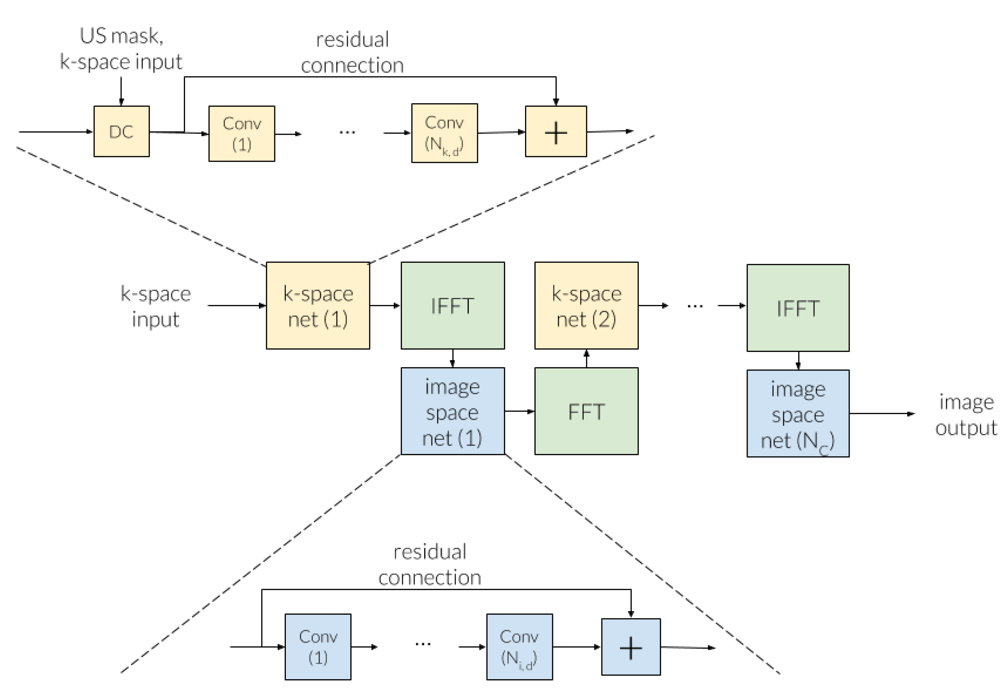
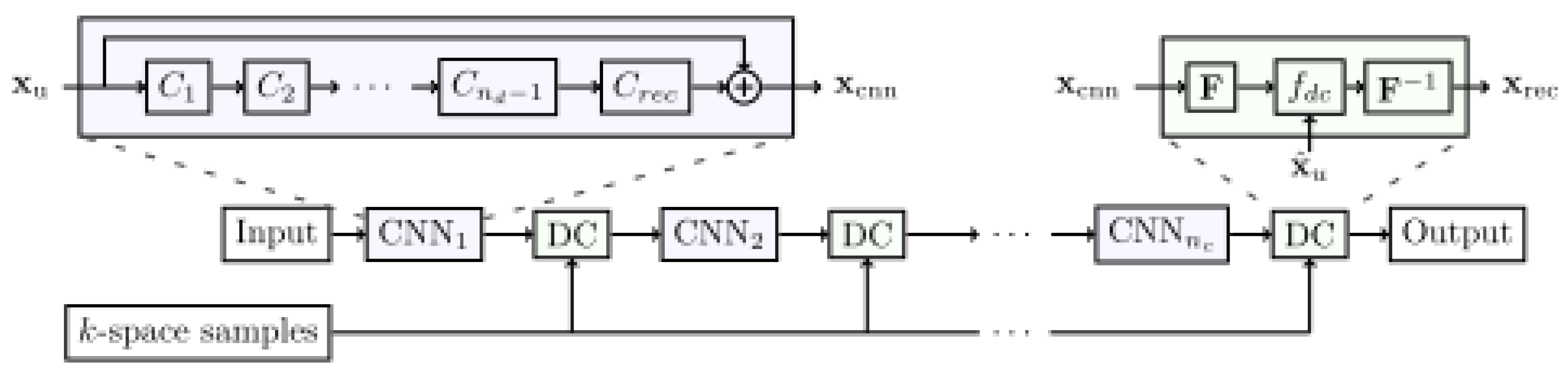
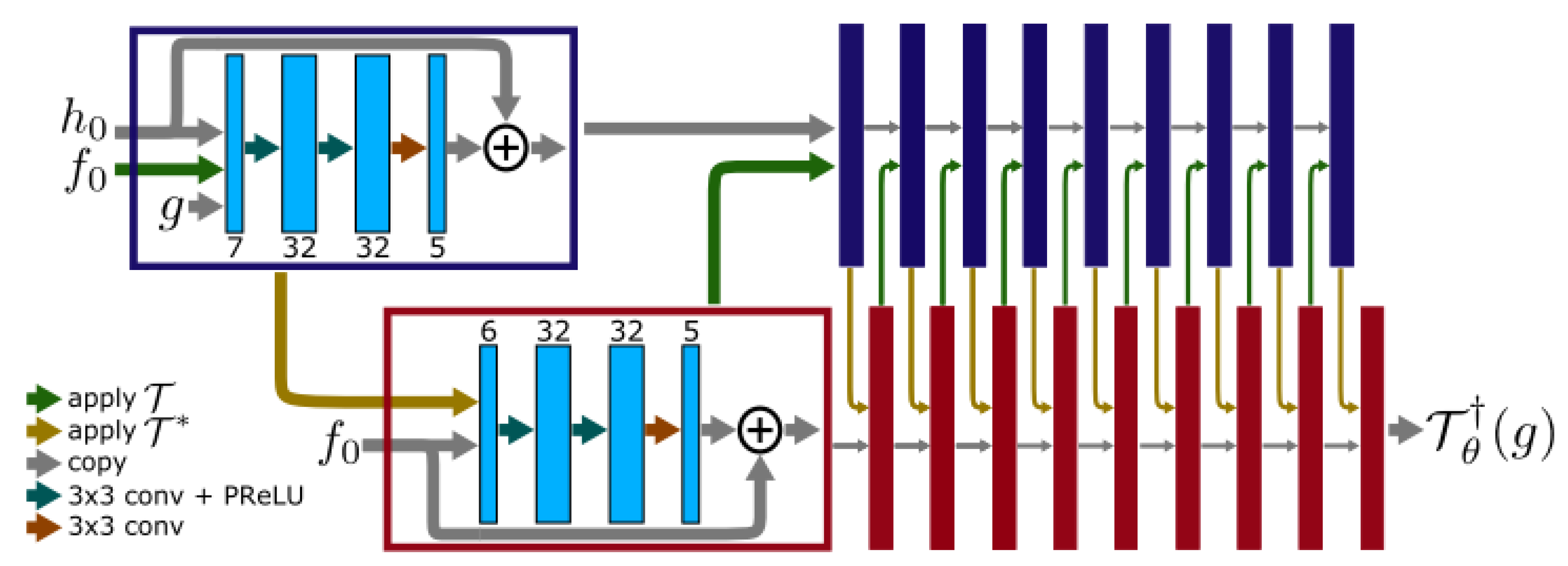
3.3.2. Cross-Domains Networks
3.4. Training
4. Data
4.1. Under-Sampling
4.2. FastMRI
4.3. OASIS
5. Results
5.1. Metrics
- The Peak Signal-to-Noise Ratio (PSNR);
- The Structural SIMilarity index (SSIM) [45];
- The number of trainable parameters in the network;
- The runtime in seconds of the neural network on a single volume.
5.2. Quantitative Results
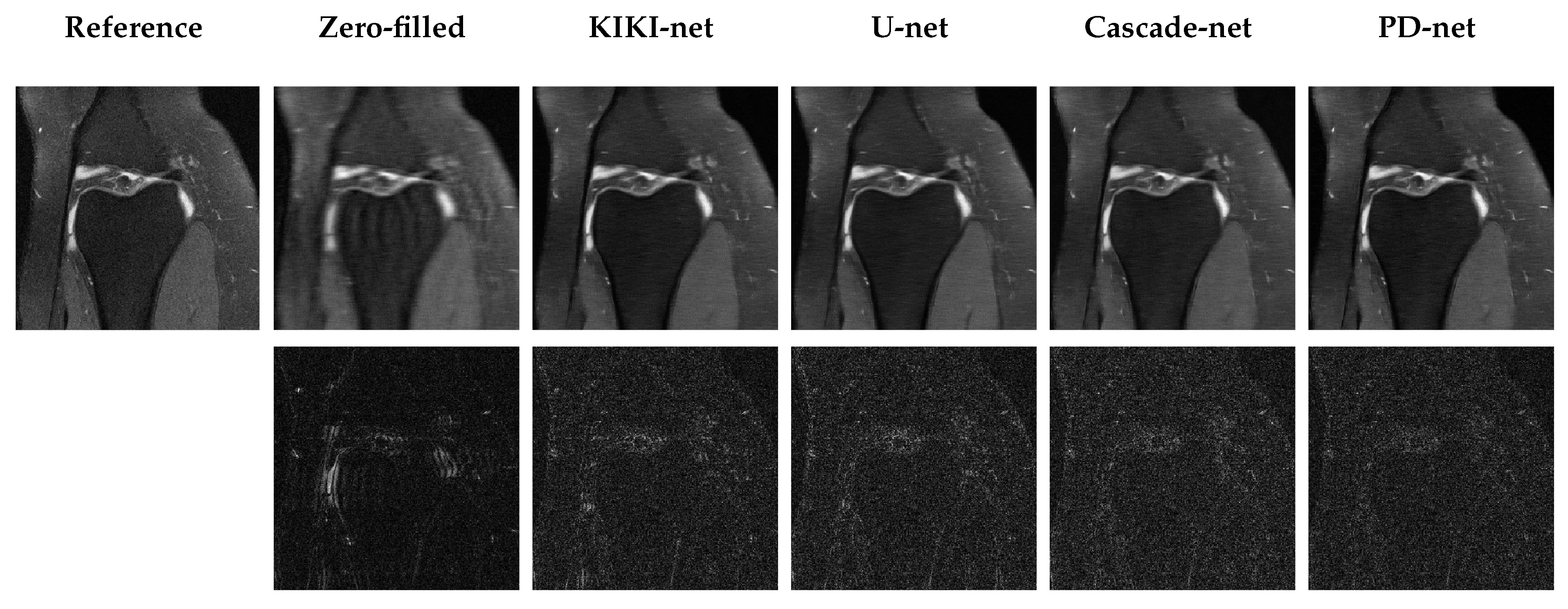
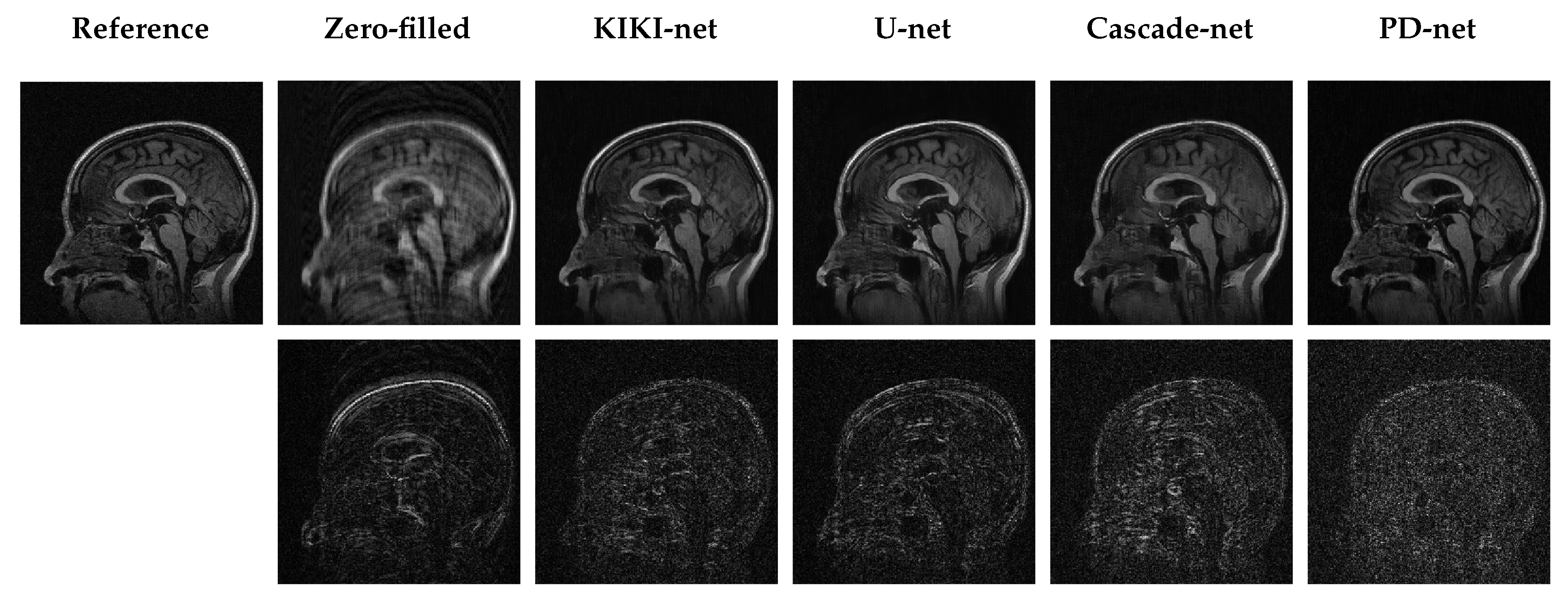
5.3. Qualitative Results
6. Discussion
Author Contributions
Funding
Acknowledgments
Conflicts of Interest
Abbreviations
| MRI | Magnetic Resonance Imaging |
| CS-MRI | Compressed Sensing MRI |
| GPU | Graphical Processing Unit |
| ReLU | Rectified Linear Unit |
| PReLU | Parametrized ReLU |
| PSNR | Peak Signal-to-Noise Ratio |
| SSIM | Structural SIMilarity index |
References
- Ramzi, Z.; Ciuciu, P.; Starck, J.L. Benchmarking Deep Nets MRI Reconstruction Models on the FastMRI Publicly Available Dataset. In Proceedings of the ISBI 2020—International Symposium on Biomedical Imaging, Iowa City, IA, USA, 3–7 April 2020. [Google Scholar]
- Smith-Bindman, R.; Miglioretti, D.L.; Larson, E.B. Rising use of diagnostic medical imaging in a large integrated health system. Health Aff. 2008, 27, 1491–1502. [Google Scholar] [CrossRef] [PubMed]
- Roemer, P.B.; Edelstein, W.A.; Hayes, C.E.; Souza, S.P.; Mueller, O.M. The NMR phased array. Magn. Reson. Med. 1990, 16, 192–225. [Google Scholar] [CrossRef] [PubMed]
- Lustig, M.; Donoho, D.; Pauly, J.M. Sparse MRI: The Application of Compressed Sensing for Rapid MR Imaging Michael. Magn. Reson. Med. 2007. [Google Scholar] [CrossRef] [PubMed]
- NHS. NHS Eebsite. Available online: https://www.nhs.uk/conditions/mri-scan/what-happens/ (accessed on 4 March 2020).
- AIM Specialty Health. Clinical Appropriateness Guidelines: Advanced Imaging. 2017. Available online: https://www.aimspecialtyhealth.com/PDF/Guidelines/2017/Sept05/AIM_Guidelines.pdf (accessed on 4 March 2020).
- Ramzi, Z.; Ciuciu, P.; Starck, J.L. Benchmarking proximal methods acceleration enhancements for CS-acquired MR image analysis reconstruction. In Proceedings of the SPARS 2019—Signal Processing with Adaptive Sparse Structured Representations Workshop, Toulouse, France, 1–4 July 2019. [Google Scholar]
- Zhu, B.; Liu, J.Z.; Cauley, S.F.; Rosen, B.R.; Rosen, M.S. Image reconstruction by domain-transform manifold learning. Nature 2018, 555, 487–492. [Google Scholar] [CrossRef] [PubMed]
- Adler, J.; Öktem, O. Learned Primal-Dual Reconstruction. IEEE Trans. Med. Imaging 2018, 37, 1322–1332. [Google Scholar] [CrossRef] [PubMed]
- Eo, T.; Jun, Y.; Kim, T.; Jang, J.; Lee, H.J.; Hwang, D. KIKI-net: Cross-domain convolutional neural networks for reconstructing undersampled magnetic resonance images. Magn. Reson. Med. 2018, 80, 2188–2201. [Google Scholar] [CrossRef]
- Schlemper, J.; Caballero, J.; Hajnal, J.V.; Price, A.; Rueckert, D. A Deep Cascade of Convolutional Neural Networks for MR Image Reconstruction. IEEE Trans. Med. Imaging 2018, 37, 491–503. [Google Scholar] [CrossRef]
- Zbontar, J.; Knoll, F.; Sriram, A.; Muckley, M.J.; Bruno, M.; Defazio, A.; Parente, M.; Geras, K.J.; Katsnelson, J.; Chandarana, H.; et al. fastMRI: An Open Dataset and Benchmarks for Accelerated MRI. arXiv 2018, arXiv:1811.08839. [Google Scholar]
- LaMontagne, P.J.; Keefe, S.; Lauren, W.; Xiong, C.; Grant, E.A.; Moulder, K.L.; Morris, J.C.; Benzinger, T.L.; Marcus, D.S. OASIS-3: Longitudinal neuroimaging, clinical, and cognitive dataset for normal aging and Alzheimer’s disease. Alzheimer’s Dementia J. Alzheimer’s Assoc. 2018, 14, P1097. [Google Scholar] [CrossRef]
- Chollet, F. Keras. 2015. Available online: https://keras.io (accessed on 4 March 2020).
- Abadi, M.; Agarwal, A.; Barham, P.; Brevdo, E.; Chen, Z.; Citro, C.; Corrado, G.S.; Davis, A.; Dean, J.; Devin, M.; et al. TensorFlow: Large-Scale Machine Learning on Heterogeneous Systems. 2015. Available online: tensorflow.org (accessed on 4 March 2020).
- Virtue, P.; Stella, X.Y.; Lustig, M. Better than real: Complex-valued neural nets for MRI fingerprinting. In Proceedings of the 2017 IEEE International Conference on Image Processing (ICIP), Beijing, China, 17–20 September 2017; pp. 3953–3957. [Google Scholar]
- Aggarwal, H.K.; Mani, M.P.; Jacob, M. Multi-Shot Sensitivity-Encoded Diffusion MRI Using Model-Based Deep Learning (Modl-Mussels). In Proceedings of the 2019 IEEE 16th International Symposium on Biomedical Imaging (ISBI 2019), Venice, Italy, 8–11 April 2019; pp. 1541–1544. [Google Scholar]
- Minh Quan, T.; Nguyen-Duc, T.; Jeong, W.K. Compressed Sensing MRI Reconstruction using a Generative Adversarial Network with a Cyclic Loss. IEEE Trans. Med. Imaging 2018, 37, 1488–1497. [Google Scholar] [CrossRef]
- Yang, Y.; Sun, J.; Li, H.; Xu, Z.; Sun, J.; Xu, Z. Deep ADMM-net for compressive sensing MRI. In Proceedings of the Neural Information Processing Systems, Barcelona, Spain, 5–10 December 2016; pp. 10–18. [Google Scholar] [CrossRef]
- Petersen, R.C.; Aisen, P.; Beckett, L.A.; Donohue, M.; Gamst, A.; Harvey, D.J.; Jack, C.; Jagust, W.; Shaw, L.; Toga, A.; et al. Alzheimer’s disease neuroimaging initiative (ADNI): Clinical characterization. Neurology 2010, 74, 201–209. [Google Scholar] [CrossRef]
- Haldar, J.P. Low-Rank Modeling of Local k-Space Neighborhoods (LORAKS) for Constrained MRI. IEEE Trans. Med. Imaging 2014, 33, 668–681. [Google Scholar] [CrossRef] [PubMed]
- Condat, L. A Primal–Dual Splitting Method for Convex Optimization Involving Lipschitzian, Proximable and Linear Composite Terms. J. Optim. Theory Appl. 2013, 158, 460–479. [Google Scholar] [CrossRef]
- Chambolle, A.; Pock, T. A First-Order Primal-Dual Algorithm for Convex Problems with Applications to Imaging. J. Math. Imaging Vis. 2011, 120–145. [Google Scholar] [CrossRef]
- Beck, A.; Teboulle, M. A fast iterative shrinkage-thresholding algorithm for linear inverse problems. SIAM J. Imaging Sci. 2009, 2, 183–202. [Google Scholar] [CrossRef]
- Kim, D.; Fessler, J.A. Adaptive restart of the optimized gradient method for convex optimization. J. Optim. Theory Appl. 2018, 178, 240–263. [Google Scholar] [CrossRef]
- Ravishankar, S.; Bresler, Y. Magnetic Resonance Image Reconstruction from Highly Undersampled K-Space Data Using Dictionary Learning. IEEE Trans. Med. Imaging 2011, 30, 1028–1041. [Google Scholar] [CrossRef]
- Caballero, J.; Price, A.N.; Rueckert, D.; Hajnal, J.V. Dictionary learning and time sparsity for dynamic MR data reconstruction. IEEE Trans. Med. Imaging 2014, 33, 979–994. [Google Scholar] [CrossRef]
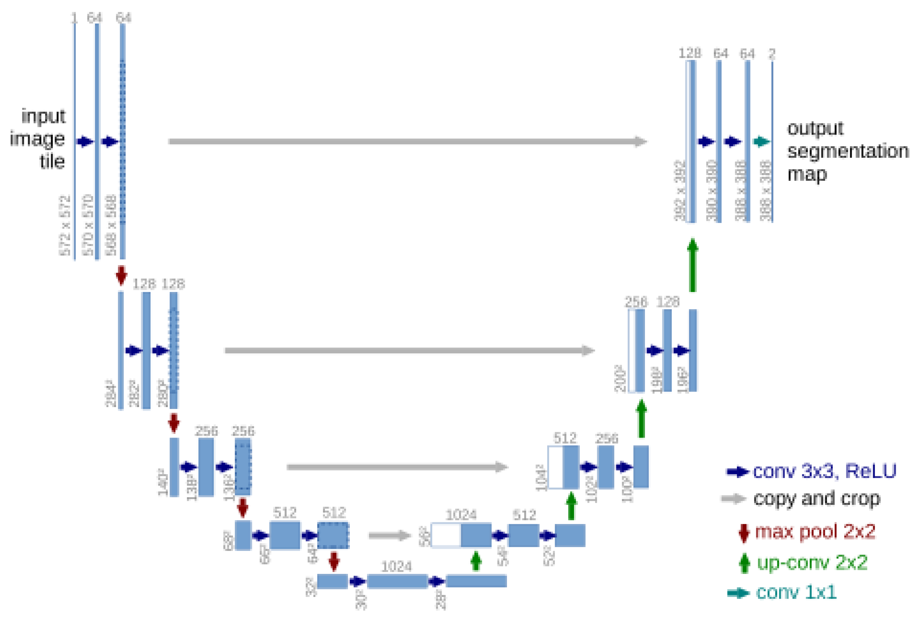
- Ronneberger, O.; Fischer, P.; Brox, T. U-Net: Convolutional Networks for Biomedical Image Segmentation. arXiv 2015, arXiv:1505.04597v1. [Google Scholar]
- Han, Y.; Sunwoo, L.; Chul Ye, J. k-Space Deep Learning for Accelerated MRI. arXiv 2019, arXiv:1805.03779v2. [Google Scholar] [CrossRef]
- Min Hyun, C.; Pyung Kim, H.; Min Lee, S.; Lee, S.; Keun Seo, J. Deep learning for undersampled MRI reconstruction. arXiv 2019, arXiv:1709.02576v3. [Google Scholar]
- Gregor, K.; Lecun, Y. Learning Fast Approximations of Sparse Coding. In Proceedings of the 27thInternational Confer-ence on Machine Learning, Haifa, Israel, 13–15 June 2010. [Google Scholar]
- Cheng, J.; Wang, H.; Ying, L.; Liang, D. Model Learning: Primal Dual Networks for Fast MR imaging. arXiv 2019, arXiv:1908.02426. [Google Scholar]
- He, K.; Zhang, X.; Ren, S.; Sun, J. Delving Deep into Rectifiers: Surpassing Human-Level Performance on ImageNet Classification. arXiv 2015, arXiv:1502.01852. [Google Scholar]
- Kingma, D.P.; Ba, J. Adam: A Method for Stochastic Optimization. arXiv 2014, arXiv:1412.6980. [Google Scholar]
- Pascanu, R.; Mikolov, T.; Bengio, Y. On the difficulty of training Recurrent Neural Networks. arXiv 2012, arXiv:1211.5063. [Google Scholar]
- Chauffert, N.; Ciuciu, P.; Kahn, J.; Weiss, P. Variable density sampling with continuous trajectories. SIAM J. Imaging Sci. 2014, 7, 1962–1992. [Google Scholar] [CrossRef]
- Irarrazabal, P.; Nishimura, D.G. Fast Three Dimensional Magnetic Resonance Imaging. Magn. Reson. Med. 1995, 33, 656–662. [Google Scholar] [CrossRef]
- Meyer, C.H.; Hu, B.S.; Nishimura, D.G.; Macovski, A. Fast Spiral Coronary Artery Imaging. Magn. Reson. Med. 1992, 28, 202–213. [Google Scholar] [CrossRef]
- Lazarus, C.; Weiss, P.; Chauffert, N.; Mauconduit, F.; El Gueddari, L.; Destrieux, C.; Zemmoura, I.; Vignaud, A.; Ciuciu, P. SPARKLING: Variable-density k-space filling curves for accelerated T 2 * -weighted MRI. Magn. Reson. Med. 2018, 1–19. [Google Scholar] [CrossRef]
- Sanchez, T.; Gözcü, B.; van Heeswijk, R.B.; Eftekhari, A.; Ilıcak, E.; Çukur, T.; Cevher, V. Scalable learning-based sampling optimization for compressive dynamic MRI. arXiv 2019, arXiv:1902.00386. [Google Scholar]
- Sherry, F.; Benning, M.; Reyes, J.C.D.l.; Graves, M.J.; Maierhofer, G.; Williams, G.; Schönlieb, C.B.; Ehrhardt, M.J. Learning the sampling pattern for MRI. arXiv 2019, arXiv:1906.08754. [Google Scholar]
- Aggarwal, H.K.; Jacob, M. J-MoDL: Joint Model-Based Deep Learning for Optimized Sampling and Reconstruction. arXiv 2019, arXiv:1911.02945. [Google Scholar]
- Wu, Y.; Rosca, M.; Lillicrap, T. Deep compressed sensing. arXiv 2019, arXiv:1905.06723. [Google Scholar]
- Weiss, T.; Senouf, O.; Vedula, S.; Michailovich, O.; Zibulevsky, M.; Bronstein, A. PILOT: Physics-Informed Learned Optimal Trajectories for Accelerated MRI. arXiv 2019, arXiv:1909.05773. [Google Scholar]
- Wang, Z.; Bovik, A.C.; Rahim Sheikh, H.; Simoncelli, E.P. Image Quality Assessment: From Error Visibility to Structural Similarity. IEEE Trans. Image Process. 2004, 13. [Google Scholar] [CrossRef]
- Horvath, K.A.; Li, M.; Mazilu, D.; Guttman, M.A.; McVeigh, E.R. Real-time magnetic resonance imaging guidance for cardiovascular procedures. In Seminars in Thoracic and Cardiovascular Surgery; Elsevier: New York, NY, USA, 2007; Volume 19, pp. 330–335. [Google Scholar]
- Schlemper, J.; Sadegh, S.; Salehi, M.; Kundu, P.; Lazarus, C.; Dyvorne, H.; Rueckert, D.; Sofka, M. Nonuniform Variational Network: Deep Learning for Accelerated Nonuniform MR Image Reconstruction. In Proceedings of the International Conference on Medical Image Computing and Computer-Assisted Intervention, Shenzhen, China, 13–17 October 2019. [Google Scholar]
- El Gueddari, L.; Ciuciu, P.; Chouzenoux, E.; Vignaud, A.; Pesquet, J.C. Calibrationless OSCAR-based image reconstruction in compressed sensing parallel MRI. In Proceedings of the 16th IEEE International Symposium on Biomedical Imaging, Venice, Italy, 8–11 April 2019; pp. 1532–1536. [Google Scholar]
- Dragotti, P.L.; Dong, H.; Yang, G.; Guo, Y.; Firmin, D.; Slabaugh, G.; Yu, S.; Keegan, J.; Ye, X.; Liu, F.; et al. DAGAN: Deep De-Aliasing Generative Adversarial Networks for Fast Compressed Sensing MRI Reconstruction. IEEE Trans. Med. Imaging 2017, 37, 1310–1321. [Google Scholar] [CrossRef]


| Network | PSNR-mean (std) (dB) | SSIM-mean (std) | #params | Runtime (s) |
|---|---|---|---|---|
| Zero-filled | 29.61 ( 5.28) | 0.657 ( 0.23) | 0 | 0.68 |
| KIKI-net | 31.38 (3.02) | 0.712 (0.13) | 1.25M | 8.22 |
| U-net | 31.78 ( 6.53) | 0.720 ( 0.25) | 482k | 0.61 |
| Cascade net | 31.97 ( 6.95) | 0.719 ( 0.27) | 425k | 3.58 |
| PD-net | 32.15 ( 6.90) | 0.729 ( 0.26) | 318k | 5.55 |
| Network | PSNR-mean (std) (dB) | SSIM-mean (std) | # params | Runtime (s) |
|---|---|---|---|---|
| Zero-filled | 28.44 (2.62) | 0.578 (0.095) | 0 | 0.41 |
| KIKI-net | 29.57 (2.64) | 0.6271 (0.10) | 1.25M | 8.88 |
| Cascade-net | 29.88 (2.82) | 0.6251 (0.11) | 425K | 3.57 |
| U-net | 29.89 (2.74) | 0.6334 (0.10) | 482K | 1.34 |
| PD-net | 30.06 (2.82) | 0.6394 (0.10) | 318K | 5.38 |
| Network | PSNR-mean (std) (dB) | SSIM-mean (std) | # params | Runtime (s) |
|---|---|---|---|---|
| Zero-filled | 30.63 (2.1) | 0.727 (0.087) | 0 | 0.52 |
| KIKI-net | 32.86 (2.4) | 0.797 (0.082) | 1.25M | 11.83 |
| U-net | 33.64 (2.6) | 0.807 (0.084) | 482K | 1.07 |
| Cascade-net | 33.98 (2.7) | 0.811 (0.086) | 425K | 4.22 |
| PD-net | 34.2 (2.7) | 0.818 (0.084) | 318280 | 6.08 |
| Network | PSNR-mean (std) (dB) | SSIM-mean (std) | # params | Runtime (s) |
|---|---|---|---|---|
| Zero-filled | 26.11 (1.45) | 0.672 (0.0307) | 0 | 0.165 |
| U-net | 29.8 (1.39) | 0.847 (0.0398) | 482k | 1.202 |
| KIKI-net | 30.08 (1.43) | 0.853 (0.0336) | 1.25M | 3.567 |
| Cascade-net | 32.0 (1.731) | 0.887 (0.0327) | 425k | 2.234 |
| PD-net | 33.22 (1.912) | 0.910 (0.0358) | 318k | 2.758 |
© 2020 by the authors. Licensee MDPI, Basel, Switzerland. This article is an open access article distributed under the terms and conditions of the Creative Commons Attribution (CC BY) license (http://creativecommons.org/licenses/by/4.0/).
Share and Cite
Ramzi, Z.; Ciuciu, P.; Starck, J.-L. Benchmarking MRI Reconstruction Neural Networks on Large Public Datasets. Appl. Sci. 2020, 10, 1816. https://doi.org/10.3390/app10051816
Ramzi Z, Ciuciu P, Starck J-L. Benchmarking MRI Reconstruction Neural Networks on Large Public Datasets. Applied Sciences. 2020; 10(5):1816. https://doi.org/10.3390/app10051816
Chicago/Turabian StyleRamzi, Zaccharie, Philippe Ciuciu, and Jean-Luc Starck. 2020. "Benchmarking MRI Reconstruction Neural Networks on Large Public Datasets" Applied Sciences 10, no. 5: 1816. https://doi.org/10.3390/app10051816
APA StyleRamzi, Z., Ciuciu, P., & Starck, J.-L. (2020). Benchmarking MRI Reconstruction Neural Networks on Large Public Datasets. Applied Sciences, 10(5), 1816. https://doi.org/10.3390/app10051816