A Novel Simplified Convolutional Neural Network Classification Algorithm of Motor Imagery EEG Signals Based on Deep Learning


Abstract
1. Introduction
2. Method
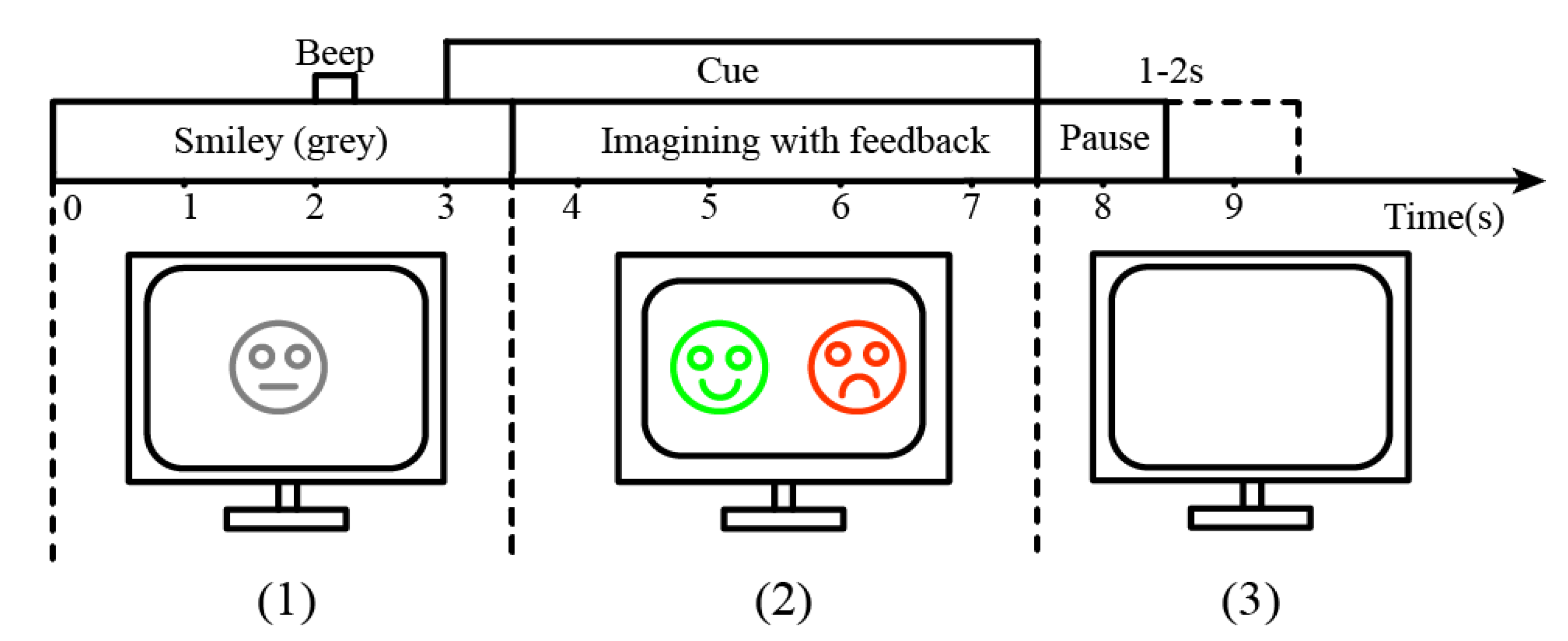
2.1. Datasets
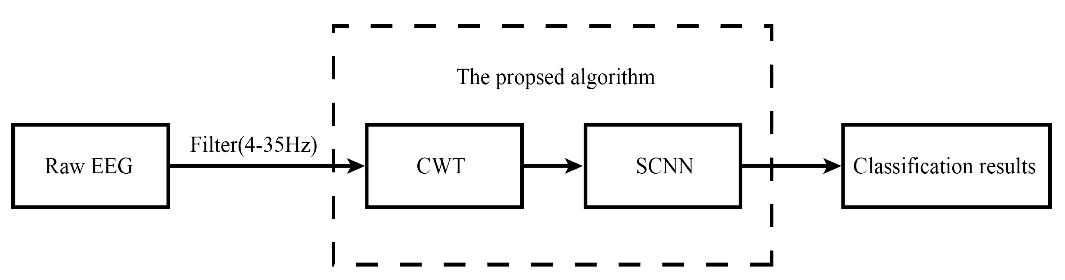
2.2. Data Analysis
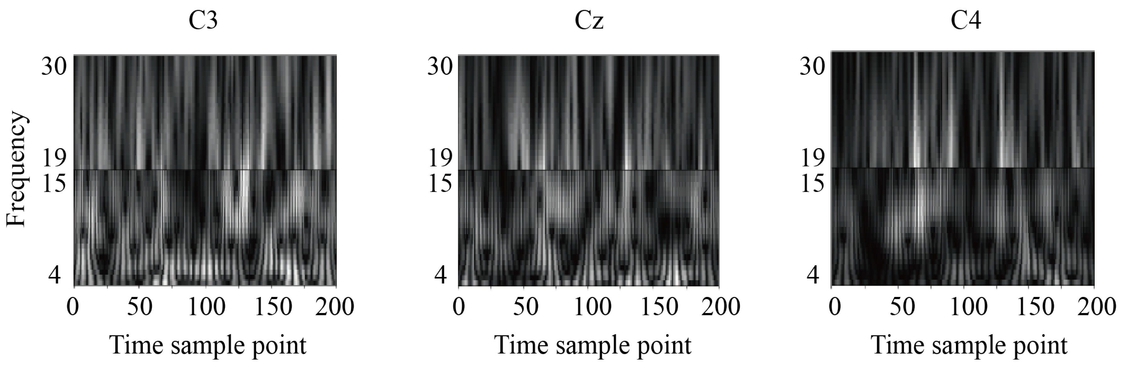
2.2.1. Continuous Wavelet Transform
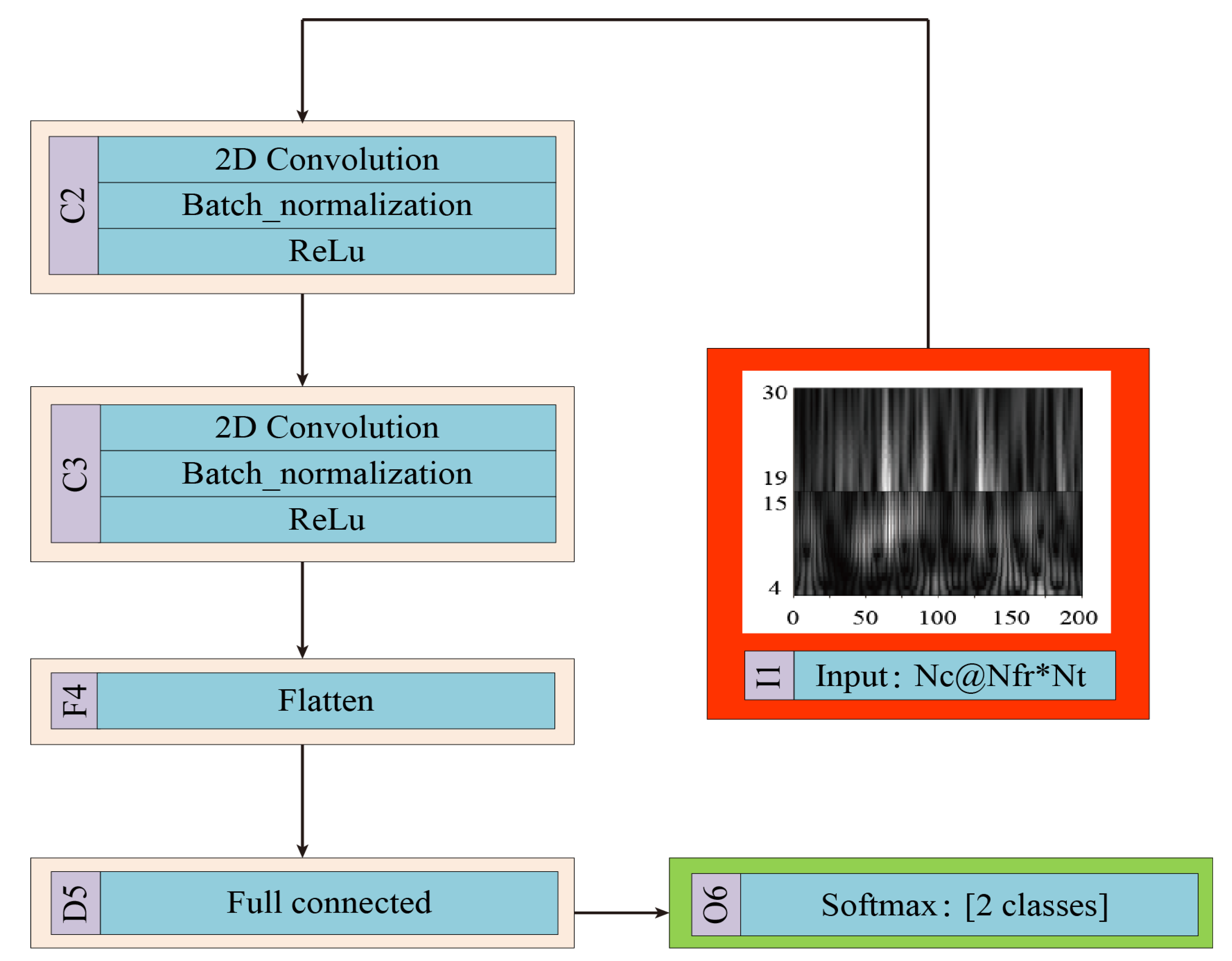
2.2.2. SCNN
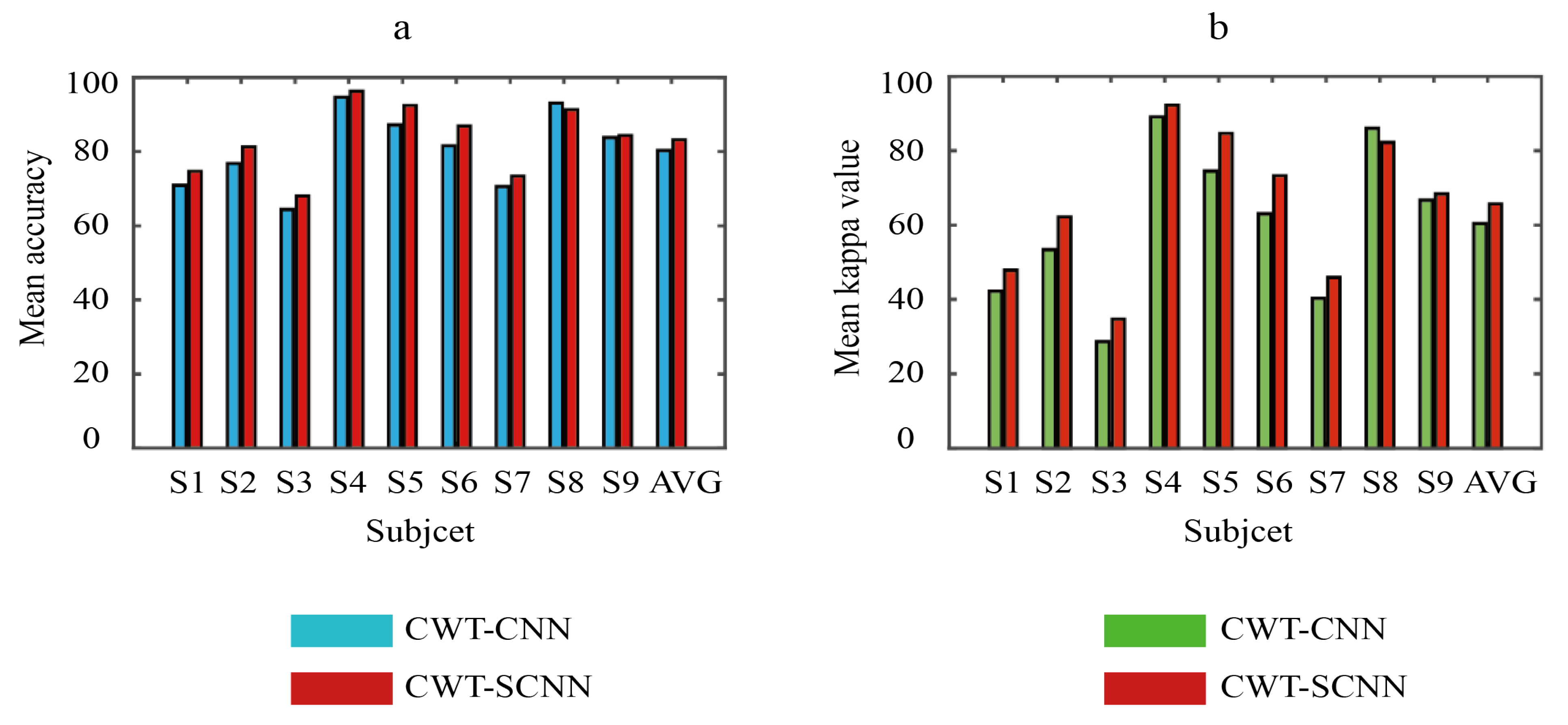
3. Experimental Results
4. Discussion
5. Conclusions
Author Contributions
Funding
Conflicts of Interest
References
- Wolpaw, J.R.; Birbaumer, N.; McFarl, D.J.; Pfurtscheller, G.; Vaughana, T.M. Brain–computer interfaces for communication and control. Clin. Neurophysiol. 2002, 113, 767–791. [Google Scholar] [CrossRef]
- Birbaumer, N.; Cohen, L.G. Brain–computer interfaces: Communication and restoration of movement in paralysis. J. Physiol. 2007, 579, 621–636. [Google Scholar] [CrossRef] [PubMed]
- Kerous, B.; Skola, F.; Liarokapis, F. EEG-based BCI and video games: A progress report. Virtual Real. 2018, 66, 2992–3005. [Google Scholar] [CrossRef]
- Kshirsagar, G.B.; Londhe, N.D. Improving performance of Devanagari script input-based P300 speller using deep learning. IEEE Trans. Biomed. Eng. 2018, 66, 2992–3005. [Google Scholar] [CrossRef] [PubMed]
- Gao, W.; Guan, J.; Gao, J.; Zhou, D. Multi-ganglion ANN based feature learning with application to P300-BCI signal classification. Biomed. Signal Process. Control 2015, 18, 127–137. [Google Scholar] [CrossRef]
- Wang, M.; Li, R.; Zhang, R.; Li, G.; Zhang, D. A wearable SSVEP-based BCI system for quadcopter control using head-mounted device. IEEE Access 2018, 6, 26789–26798. [Google Scholar] [CrossRef]
- Kwak, N.S.; Müller, K.R.; Lee, S.W. A convolutional neural network for steady state visual evoked potential classification under ambulatory environment. PLoS ONE 2017, 12, e0172578. [Google Scholar] [CrossRef]
- Lu, N.; Li, T.; Ren, X.; Miao, H.Y. A deep learning scheme for motor imagery classification based on restricted boltzmann machines. IEEE Trans. Neural Syst. Rehabil. Eng. 2016, 25, 566–576. [Google Scholar] [CrossRef]
- Ma, T.; Li, H.; Yang, H.; Lv, X.; Li, P.; Yao, D. The extraction of motion-onset VEP BCI features based on deep learning and compressed sensing. J. Neurosci. Methods 2017, 275, 80–92. [Google Scholar] [CrossRef]
- Müller, K.R.; Tangermann, M.; Dornhege, G.; Krauledat, M.; Curio, G.; Blankertz, B. Machine learning for real-time single-trial EEG-analysis: From brain–computer interfacing to mental state monitoring. J. Neurosci. Methods 2008, 167, 82–90. [Google Scholar] [CrossRef]
- Acharya, R.; Faust, O.; Kannathal, N.; Chua, T.; Laxminarayan, S. Non-linear analysis of EEG signals at various sleep stages. Comput. Methods Programs Biomed. 2005, 80, 37–45. [Google Scholar] [CrossRef] [PubMed]
- Tang, X.; Li, W.; Li, X.; Ma, Z.; Dang, X. Motor imagery EEG recognition based on conditional optimization empirical mode decomposition and multi-scale convolutional neural network. Expert Syst. Appl. 2020, 149, 113285. [Google Scholar] [CrossRef]
- Wu, S.L.; Wu, C.W.; Pal, N.R.; Chen, C.; Chen, S.; Lin, C. Common spatial pattern and linear discriminant analysis for motor imagery classification. In Proceedings of the 2013 IEEE Symposium on Computational Intelligence, Cognitive Algorithms, Mind, and Brain, Singapore, 16–19 April 2013. [Google Scholar]
- Liu, Z.; Lai, Z.; Ou, W.; Zhang, K.; Zheng, R. Structured optimal graph based sparse feature extraction for semi-supervised learning. Signal Process. 2020, 170, 107456. [Google Scholar] [CrossRef]
- Ruan, J.; Wu, X.; Zhou, B.; Guo, X.; Lv, Z. An Automatic Channel Selection Approach for ICA-Based Motor Imagery Brain Computer Interface. J. Med. Syst. 2018, 42, 253. [Google Scholar] [CrossRef] [PubMed]
- Sakhavi, S.; Guan, C.; Yan, S. Parallel convolutional-linear neural network for motor imagery classification. In Proceedings of the 2015 23rd European Signal Processing Conference (EUSIPCO), Nice, France, 1–4 September 2015. [Google Scholar]
- Dose, H.; Møller, J.S.; Iversen, H.K.; Puthusserypady, S. An end-to-end deep learning approach to MI-EEG signal classification for BCIs. Expert Syst. Appl. 2018, 114, 532–542. [Google Scholar] [CrossRef]
- Sturm, I.; Lapuschkin, S.; Samek, W.; Müller, K.R. Interpretable deep neural networks for single-trial EEG classification. J. Neurosci. Methods 2016, 274, 141–145. [Google Scholar] [CrossRef]
- Zhang, R.; Zong, Q.; Dou, L. A novel hybrid deep learning scheme for four-class motor imagery classification. J. Neural Eng. 2019, 16, 066004. [Google Scholar] [CrossRef]
- Li, M.A.; Zhang, M.; Sun, Y.J. A novel motor imagery EEG recognition method based on deep learning. In Proceedings of the 2016 International Forum on Management, Education and Information Technology Application, Guangzhou, China, 30–31 January 2016. [Google Scholar]
- Tang, Z.; Li, C.; Sun, S. Single-trial EEG classification of motor imagery using deep convolutional neural networks. Opt.-Int. J. Light Electron Opt. 2017, 130, 11–18. [Google Scholar] [CrossRef]
- Tabar, Y.R.; Halici, U. A novel deep learning approach for classification of EEG motor imagery signals. J. Neural Eng. 2016, 14, 016003. [Google Scholar] [CrossRef]
- Adeli, H.; Zhou, Z.; Dadmehr, N. Analysis of EEG records in an epileptic patient using wavelet transform. J. Neurosci. Methods 2003, 123, 69–87. [Google Scholar] [CrossRef]
- LeCun, Y.; Bengio, Y.; Hinton, G. Deep learning. Nature 2013, 521, 436–444. [Google Scholar] [CrossRef] [PubMed]
- Xiang, L.; Guo, G.; Yu, J.; Sheng, V.; Yang, P. A convolutional neural network-based linguistic steganalysis for synonym substitution steganography. Math. Biosci. Eng. 2020, 17, 1041–1058. [Google Scholar] [CrossRef]
- Strubell, E.; Ganesh, A.; McCallum, A. Energy and policy considerations for deep learning in NLP. arXiv 2019, arXiv:1906.02243. [Google Scholar]
- González-Briones, A.; Villarrubia, G.; De Paz, J.F.; Corchado, J.M. A multi-agent system for the classification of gender and age from images. Comput. Vis. Image Underst. 2018, 172, 98–106. [Google Scholar] [CrossRef]
- Zhang, D.; Yang, G.; Li, F.; Sangaiah, A.K. Detecting seam carved images using uniform local binary patterns. Multimedia Tools Appl. 2018, 18, 1–16. [Google Scholar] [CrossRef]
- Dai, M.; Zheng, D.; Na, R.; Wang, S.; Zhang, S. EEG classification of motor imagery using a novel deep learning framework. Sensors 2019, 19, 551. [Google Scholar] [CrossRef]
- Tavanaei, A.; Ghodrati, M.; Kheradpisheh, S.R.; Masquelier, T.; Maida, A. Deep learning in spiking neural networks. Neural Netw. 2019, 111, 47–63. [Google Scholar] [CrossRef]
- Saxe, A.M.; Bansal, Y.; Dapello, J.; Kolchinsky, A.; Tracey, B.D. On the information bottleneck theory of deep learning. J. Stat. Mech. Theory Exp. 2019, 2019, 124020. [Google Scholar] [CrossRef]
- Liu, M.; Wu, W.; Gu, Z. Deep learning based on Batch Normalization for P300 signal detection. Neurocomputing 2018, 275, 288–297. [Google Scholar] [CrossRef]
- Maddula, R.; Stivers, J.; Mousavi, M.; Ravindran, S. Deep Recurrent Convolutional Neural Networks for Classifying P300 BCI signals. In Proceedings of the GBCIC, Graz, Austria, 18–22 September 2017. [Google Scholar]
- Aznan, N.K.N.; Bonner, S.; Connolly, J.; Moubayed, N.; Breckon, T. On the classification of SSVEP-based dry-EEG signals via convolutional neural networks. In Proceedings of the 2018 IEEE International Conference on Systems, Man, and Cybernetics, Miyazaki, Japan, 7–10 October 2018. [Google Scholar]
- Kumar, S.; Sharma, A.; Mamun, K.; Tsunoda, T. A deep learning approach for motor imagery EEG signal classification. In Proceedings of the 2016 3rd Asia-Pacific World Congress on Computer Science and Engineering, Nadi, Fiji, 5–6 December 2016. [Google Scholar]
- Tayeb, Z.; Fedjaev, J.; Ghaboosi, N.; Richter, C.; Everding, L. Validating deep neural networks for online decoding of motor imagery movements from EEG signals. Sensors 2019, 19, 210. [Google Scholar] [CrossRef]
- Li, M.; Zhu, W.; Zhang, M.; Sun, Y.; Wang, Z. The novel recognition method with optimal wavelet packet and LSTM based recurrent neural networkIn Proceedings of the IEEE International Conference on Mechatronics and Automation, Ningbo, China, 19–21 November 2017.
- Pfurtscheller, G.; Neuper, C.; Flotzinger, D.; Pregenzer, M. EEG-based discrimination between imagination of right and left hand movement. Electroencephalogr. Clin. Neurophysiol. 1997, 103, 642–651. [Google Scholar] [CrossRef]
- Sethi, S.; Upadhyay, R.; Singh, H.S. Stockwell-common spatial pattern technique for motor imagery-based Brain Computer Interface design. Comput. Electr. Eng. 2018, 71, 492–504. [Google Scholar] [CrossRef]
- Qiu, Z.; Allison, B.Z.; Jin, J.; Zhang, Y.; Wang, X.; Li, W.; Cichocki, A. Optimized motor imagery paradigm based on imagining Chinese characters writing movement. IEEE Trans. Neural Syst. Rehabil. Eng. 2017, 25, 1009–1017. [Google Scholar] [CrossRef] [PubMed]
- Cun, Y.L.; Boser, B.; Denker, J.S.; Henderson, D.; Howard, R.E.; Hubbard, W.E.; Jackel, L.D. Handwritten Digit Recognition with a Back-Propagation Network. Adv. Neural Inf. Process. Syst. 1997, 2, 396–404. [Google Scholar]
- Hanin, B. Universal function approximation by deep neural nets with bounded width and relu activations. Mathematics 2019, 7, 992. [Google Scholar] [CrossRef]
- Zhang, J.; Bargal, S.A.; Lin, Z.; Brandt, J.; Shen, X.; Sclaroff, S. Top-down neural attention by excitation backprop. Int. J. Comput. Vis. 2018, 126, 1084–1102. [Google Scholar] [CrossRef]
- Sun, S.; Zhou, J. A review of adaptive feature extraction and classification methods for EEG-based brain-computer interfaces. In Proceedings of the 2014 International Joint Conference on Neural Networks (IJCNN), Beijing, China, 6–11 July 2014. [Google Scholar]
- An, X.; Kuang, D.; Guo, X.; Zhao, Y. A deep learning method for classification of EEG data based on motor imagery. In Proceedings of the International Conference on Intelligent Computing, Taiyuan, China, 3–6 August 2014; pp. 203–210. [Google Scholar]
- Blankertz, B.; Tomioka, R.; Lemm, S.; Kawanabe, M.; Muller, K.R. Optimizing Spatial filters for Robust EEG Single-Trial Analysis. IEEE Signal Process. Mag. 2008, 25, 41–56. [Google Scholar] [CrossRef]
- Li, M.; Liu, Y.; Wu, Y.; Liu, S.; Jia, J.; Zhang, L. Neurophysiological substrates of stroke patients with motor imagery-based brain-computer interface training. Int. J. Neurosci. 2014, 124, 403–415. [Google Scholar]
- Ono, T.; Kimura, A.; Ushiba, J. Daily training with realistic visual feedback improves reproducibility of event-related desynchronisation following hand motor imagery. Clin. Neurophysiol. 2013, 124, 1779–1786. [Google Scholar] [CrossRef]
- Hsu, W.Y.; Sun, Y.N. EEG-based motor imagery analysis using weighted wavelet transform features. J. Neurosci. Methods 2009, 176, 310–318. [Google Scholar] [CrossRef]
- Ma, L.; Stückler, J.; Wu, T.; Cremers, D. Detailed Dense Inference with Convolutional Neural Networks via Discrete Wavelet Transform. arXiv 2018, arXiv:1808.01834. [Google Scholar]


| Short Name | Layer (Type) | Output Shape | Parameter |
|---|---|---|---|
| I1 | Input layer | (44, 200, 3) | None |
| C2 | Convolution layer | (1, 200, 8) | 1064 |
| Batch normalization layer | (1, 200, 8) | 4 | |
| Activation layer | (1, 200, 8) | None | |
| C3 | Convolution layer | (1, 20, 16) | 1296 |
| Batch normalization layer | (1, 20, 16) | 64 | |
| Activation layer | (1, 20, 16) | None | |
| F4 | Flatten layer | (none, 320) | None |
| D5 | Fully connected layer | (none, 64) | 20,544 |
| O6 | Output layer | (none, 2) | 130 |
| Subject | Classification Accuracy (%) | ||||
|---|---|---|---|---|---|
| CNN-SAE | CSP | ACSP | DBN | CWT-SCNN | |
| S1 | 76.0 | 66.6 | 67.5 | 66.6 | 74.7 |
| S2 | 65.8 | 57.9 | 55.4 | 62.5 | 81.3 |
| S3 | 75.3 | 61.3 | 62.2 | 60.0 | 68.1 |
| S4 | 95.3 | 94.0 | 94.7 | 96.8 | 96.3 |
| S5 | 83.0 | 80.6 | 76.9 | 82.0 | 92.5 |
| S6 | 79.5 | 75.0 | 75.9 | 77.4 | 86.9 |
| S7 | 74.5 | 72.5 | 71.3 | 76.6 | 73.4 |
| S8 | 75.3 | 89.4 | 89.4 | 88.8 | 91.6 |
| S9 | 73.3 | 85.6 | 81.3 | 86.0 | 84.4 |
| Average | 77.6 | 75.9 | 75.0 | 77.4 | 83.2 |
| Subject | Kappa Value | ||||
|---|---|---|---|---|---|
| CNN-SAE | CSP | ACSP | DBN | CWT-SCNN | |
| S1 | 0.488 | 0.312 | 0.332 | 0.302 | 0.478 |
| S2 | 0.289 | 0.192 | 0.163 | 0.218 | 0.622 |
| S3 | 0.427 | 0.206 | 0.215 | 0.209 | 0.347 |
| S4 | 0.888 | 0.907 | 0.915 | 0.929 | 0.923 |
| S5 | 0.593 | 0.632 | 0.548 | 0.648 | 0.847 |
| S6 | 0.495 | 0.521 | 0.546 | 0.567 | 0.733 |
| S7 | 0.409 | 0.507 | 0.498 | 0.545 | 0.459 |
| S8 | 0.443 | 0.798 | 0.806 | 0.774 | 0.822 |
| S9 | 0.415 | 0.724 | 0.715 | 0.731 | 0.684 |
| Average | 0.547 | 0.533 | 0.526 | 0.547 | 0.657 |
| Subject | Mean Classification Accuracy (%) | |||
|---|---|---|---|---|
| CSP-SCNN | FFT-SCNN | STFT-SCNN | CWT-SCNN | |
| S1 | 65.0 | 69.1 | 72.5 | 74.7 |
| S2 | 74.4 | 72.8 | 80.0 | 81.3 |
| S3 | 64.7 | 67.8 | 64.4 | 68.1 |
| S4 | 95.6 | 94.4 | 96.3 | 96.3 |
| S5 | 83.8 | 88.1 | 88.8 | 92.5 |
| S6 | 72.5 | 72.2 | 71.6 | 86.9 |
| S7 | 67.2 | 67.5 | 66.3 | 73.4 |
| S8 | 92.5 | 90.0 | 91.9 | 91.3 |
| S9 | 84.4 | 82.2 | 80.6 | 84.4 |
| Average | 77.8 | 78.2 | 79.2 | 83.2 |
| Subject | Mean Kappa Value | |||
|---|---|---|---|---|
| CSP-SCNN | FFT-SCNN | STFT-SCNN | CWT-SCNN | |
| S1 | 0.286 | 0.364 | 0.453 | 0.478 |
| S2 | 0.465 | 0.463 | 0.599 | 0.622 |
| S3 | 0.296 | 0.341 | 0.299 | 0.347 |
| S4 | 0.905 | 0.887 | 0.923 | 0.923 |
| S5 | 0.666 | 0.754 | 0.769 | 0.847 |
| S6 | 0.448 | 0.410 | 0.443 | 0.733 |
| S7 | 0.344 | 0.358 | 0.330 | 0.459 |
| S8 | 0.848 | 0.794 | 0.829 | 0.822 |
| S9 | 0.685 | 0.640 | 0.618 | 0.684 |
| Average | 0.549 | 0.556 | 0.585 | 0.657 |
| Short Name | Layer (Type) | Output Shape | Parameter |
|---|---|---|---|
| I1 | Input layer | (44, 200, 3) | None |
| C2 | Convolution layer | (1, 200, 8) | 1064 |
| Batch normalization layer | (1, 200, 8) | 32 | |
| Activation layer | (1, 200, 8) | None | |
| P3 | MaxPooling layer | (1, 100, 8) | None |
| C4 | Convolution layer | (1, 91, 16) | 1296 |
| Batch normalization layer | (1, 91, 16) | 64 | |
| Activation layer | (1, 91, 16) | None | |
| P5 | MaxPooling layer | (1, 46, 16) | None |
| F6 | Flatten layer | (none, 736) | None |
| D7 | Fully connected layer | (none, 64) | 47,168 |
| O8 | Output layer | (none, 2) | 130 |
© 2020 by the authors. Licensee MDPI, Basel, Switzerland. This article is an open access article distributed under the terms and conditions of the Creative Commons Attribution (CC BY) license (http://creativecommons.org/licenses/by/4.0/).
Share and Cite
Li, F.; He, F.; Wang, F.; Zhang, D.; Xia, Y.; Li, X. A Novel Simplified Convolutional Neural Network Classification Algorithm of Motor Imagery EEG Signals Based on Deep Learning. Appl. Sci. 2020, 10, 1605. https://doi.org/10.3390/app10051605
Li F, He F, Wang F, Zhang D, Xia Y, Li X. A Novel Simplified Convolutional Neural Network Classification Algorithm of Motor Imagery EEG Signals Based on Deep Learning. Applied Sciences. 2020; 10(5):1605. https://doi.org/10.3390/app10051605
Chicago/Turabian StyleLi, Feng, Fan He, Fei Wang, Dengyong Zhang, Yi Xia, and Xiaoyu Li. 2020. "A Novel Simplified Convolutional Neural Network Classification Algorithm of Motor Imagery EEG Signals Based on Deep Learning" Applied Sciences 10, no. 5: 1605. https://doi.org/10.3390/app10051605
APA StyleLi, F., He, F., Wang, F., Zhang, D., Xia, Y., & Li, X. (2020). A Novel Simplified Convolutional Neural Network Classification Algorithm of Motor Imagery EEG Signals Based on Deep Learning. Applied Sciences, 10(5), 1605. https://doi.org/10.3390/app10051605