Abstract
Noise energetic indicators, like Lden, show good correlations with long term annoyance, but should be supplemented by other parameters describing the sound fluctuations, which are very common in urban areas and negatively impact noise annoyance. Thus, in this paper, the hourly values of continuous equivalent level LAeqh and the intermittency ratio (IR) were both considered to describe the urban road traffic noise, monitored in 90 sites in the city of Milan and covering different types of road, from motorways to local roads. The noise data have been processed by clustering methods to detect similarities and to figure out a criterion to classify the urban sites taking into account both equivalent noise levels and road traffic noise events. Two clusters were obtained and, considering the cluster membership of each site, the decimal logarithm of the day-time (06:00–22:00) traffic flow was used to associate each new road with the clusters. In particular, roads with average day-time hourly traffic flow ≥1900 vehicles/hour were associated with the cluster with high traffic flow. The described methodology could be fruitfully applied on road traffic noise data in other cities.
1. Introduction
According to the data provided by the European Environment Agency (EAA), “more than 41 million people are reported to be exposed above 55 dB Lden due to road traffic noise inside urban areas”, and nearly 90 million are estimated in Europe []. Road traffic noise is the most diffuse noise source in urban areas, wide spreading in space and time, despite the noise reduction actions implemented by policies and legislations at international and national level. As a consequence, the people’s awareness towards the adverse health effects, both direct and indirect, produced by road traffic noise is increasing. The World Health Organization (WHO) has estimated that “at least one million healthy life years are lost every year from traffic related noise in the western part of Europe” []. There is evidence in the literature that “sleep disturbance and annoyance, mostly related to road traffic noise, comprise the main burden of environmental noise” [].
Lden, introduced by the European Directive 2002/49/EC on the assessment and management of environmental noise [], is commonly applied by legislation to assess urban sound environments. However, although energetic indicators show good correlations with long term annoyance, their deficiency for evaluating perceptively urban sound environments has been pointed out in several studies []. In particular, they fail in evaluating fluctuating sounds, which are very common in urban areas and negatively impact noise annoyance. Road traffic noise is typically characterized by the noise events owing to the single vehicle pass-by, where the temporal structure of sound pressure level (SPL) varies between local one-lane city roads, showing highly intermittent noise, up to wide multi-lane motorways, producing a nearly continuous noise with very limited fluctuations. There is clear evidence in the literature that human hearing is able to adapt to steady noise easier than to SPL fluctuations, as well as to prominent, salient noise events [,]. The higher these fluctuations are, the more annoying a sound is possibly perceived. To quantify these SPL fluctuations and variations, common approaches either apply thresholds to detect events exceeding such thresholds and count the number and the duration of these events, or use SPL statistics, like percentile levels LA1, LA5, and LA10, namely the A-weighted SPL exceeding for 1%, 5%, and 10% of the measurement time, respectively. Recently, a new descriptor has been proposed [], describing the eventfulness (or intermittency) of noise exposure, taking into account both the number and the magnitude of noise events during a certain time period. The metric, named the intermittency ratio (IR), accounts for all sound energy contributions that exceed a given threshold and, by definition, only takes on values between 0% and 100%. It can be derived either directly from acoustic measurements or calculated from traffic and geometric data for any transportation noise source and any time period. However, as pointed out in [,], IR could be a supplementary metric accompanying the continuous equivalent level (LAeq), which measures the energy content of the noise exposure.
The present paper starts from the results obtained in a previous application of IR on the noise data from road traffic, monitored continuously for 24 h in 90 sites in the city of Milan [,]. The database comprised 251 24-h long time series of 1 s A-weighted SPL, monitored at different types of roads, from motorways to local roads with very low traffic flow. The hourly values of LAeqh, each referring to the corresponding day-time LAeqd (06:00–22:00), and IR were computed and processed by clustering methods to figure out a criterion to classify the urban sites considering road traffic noise features. Two clusters were determined and a “non-acoustic” parameter “x”, namely the decimal logarithm of the day-time traffic flow (06:00–22:00), was taken as a binary classifier to associate each site within a group. The resulting classification was compared with the clusters obtained by k-means and the percentage of agreement was 71.9%.
2. Materials and Methods
2.1. Acoustic Data Set
Road traffic noise monitoring in Milan has a long-standing tradition, leading to a large database across the years. From this database, a set of 90 sites was considered to represent the different types of roads according to the Italian road functional classification, that is, motorway (class “A”), thoroughfare roads (class “D”), urban district roads (class “E”), and urban local roads (class “F”). The selected roads sample is representative of the urban road network in Milan and its spatial distribution of road types in the urban area is given in Figure 1.
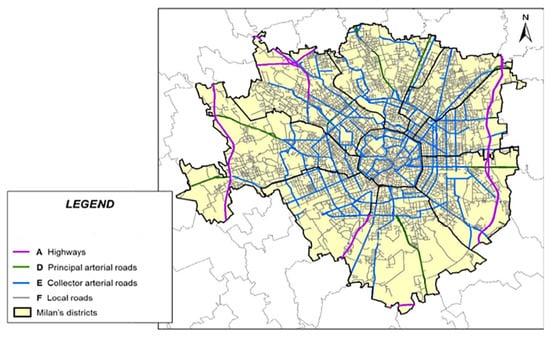
Figure 1.
The spatial distribution of road types in the urban area of Milan.
The distribution of the sites across road types is given in Table 1, together with the number of 24-h time series of 1 s A-weighted SPL, monitored continuously by a class 1 sound level meter Larson Davis 831 with the microphone placed at 4 m above the road. In some sites, the unattended monitoring was performed on more consecutive days, that is, multiple 24 h time series were available and all were averaged. The monitoring was performed on weekdays only (Monday to Friday), without rain and with wind speed less than 5 m/s. Noise events not associated with road traffic were visually detected in the SPL time histories and masked before further data processing. The microphone was placed close to the road to reduce the influence of noise from sources different from road traffic.

Table 1.
Distribution of the 90 sites considered in the study according to the Italian legislative classification of roads.
In addition, for each site, the hourly traffic flow was provided by the Municipal Agency of Mobility, Environment, and Land of Milan (AMAT). The data were calculated by a model of traffic based on origin–destination matrices and applied to the city road network.
2.2. Data Processing and Analysis
A script running in “R” environment, version 3.5.1 [], was written to import each of the 24 h time series as input in terms of text file (four columns with date, time, SPL dB(A) at 1 s intervals, and a code to indicate whether the source was road traffic or something different). In order to provide indicators for the classification, a time window of duration T = 1 hour was chosen to compute LAeq and IR values This time period was established by the Italian legislation for road traffic noise measurement. Besides this requirement, the chosen measurement time T was considered a reasonable compromise between longer time (i.e., 24 hours, day and night periods, and so on) and shorter ones (i.e., 30 min or even shorter). For the sites where the noise monitoring lasted more days, the median value of IR and LAeq for each hour was determined, as this parameter is less influenced than the mean by the presence of outliers.
From the input data, the script was computed for each hour:
- The IR value, according to the definition given in [] and determined by the following:where Leq,T,Events accounts for all sound energy contributions that exceed a given threshold K, that is, clearly standing out from background noise; Leq,T,tot is the overall continuous equivalent level referred to the measurement time T; and the threshold K is given by the following:where C, as stated in [], can be assumed equal to 3 as a result of the numerical simulations for different traffic situations;
- The LAeqh referred to the corresponding day-time LAeqd (06:00–22:00), taken as a reference level, that is, the difference δ = LAeqh − LAeqd; this computation was necessary because of the different monitoring set-up at the sites, such as different distances from the road and the characteristics of the road itself (its geometry, the presence of reflecting surfaces and obstacles in sound propagation, and types of paving) [].
As explained in Section 2.1, the microphone was placed close to the road to reduce the influence of noise from other sources and, therefore, the source–receiver distance was not always the same. This factor influences the IR values (Figure 4 in []).
Thus, a matrix formed by 48 variables, (IR and δ for each hour) × 90 observations (sites) = 4320 values, was the input of the subsequent cluster analysis, an unsupervised machine-learning technique, performed to find out similarities in the time patterns. Because the data are measured by different scales, namely δ is in dB and IR in percentage, they needed to be scaled (mean = 0 and standard deviation = 1) before clustering; in addition, the Euclidean distance, one of the most used distance metrics, was considered to represent the similarity between pairs of sites. To select the optimal solution for clustering, that is, the agglomeration algorithm and number of clusters, the “clValid” R package, version 0.6–6 [] was applied. All 10 clustering methods available in the package were considered, that is, hierarchical clustering with the Ward’s method [], partitioning around medoids (PAM) [], k-means [], DIvisive ANAlysis clustering (DIANA) [], Clustering LARge Applications (CLARA) [], AGglomerative NESting (AGNES) [], self-organizing map (SOM) [], self organizing tree algorithm (SOTA) [], model-base clustering [], and fuzzy analysis clustering []. The clustering performance of the methods was ranked according to seven internal clustering validation measures [,], namely, the connectivity [], silhouette width [] and Dunn index (combining measures of compactness and separation of the clusters) [], average proportion of non-overlap (APN), average distance (AD), average distance between means (ADM), and figure of merit (FOM) [,]. All of the clustering algorithms were ranked based on their performance as determined simultaneously by all the validation measures [].
There is no generally accepted rule on the ratio between the number of clustering variables and sample size (number of observations, sites in this study). Usually, the latter should be much higher than the former. In this study, the ratio between sites and variables is low (90/48 = 1.875). Thus, principal component analysis (PCA) was also performed on the input matrix in order to reduce the number of variables and account for the largest possible variance of the original variables. The method generates a new set of variables, called principal components, and each principal component is a linear combination of the original variables. All the principal components are orthogonal to each other, so there is no redundant information. Components with larger variance are the most relevant to the clustering and, therefore, removing features with low variance acts as a filter that results in a distance metric that provides a more robust clustering. The PCA output for the selected components was taken as input for a further k-means clustering, and the obtained classification was compared with that obtained by the earlier k-means applied to all 48 variables.
Furthermore, the hourly values of the 24 h pattern, corresponding to the cluster membership of the site, were compared with those observed at the site itself and the differences ε were evaluated in terms of root mean square (RMS) and probability Pε of ε being within a specified interval width.
Supervised machine-learning algorithms can be applied to classify new roads into the clusters determined by the cluster analysis, but the acoustic data must be known. Unfortunately, very often they are not available and, therefore, an alternative classifier is needed. For this purpose, the road traffic flow is a potential candidate as its value, obtained from transport models or measured, is rather available and linked to the produced noise. In the present study, the decimal logarithm of the day-time (06:00–22:00) traffic flow rate was considered as an alternative road classifier.
3. Results
3.1. Determination of Clusters and Patterns of Hourly Values of δ and IR
The clustering algorithms ranking based on their performance as determined by all the validation measures showed that the best solution was the k-means agglomeration algorithm, a centroid-based clustering, and a division into two clusters. The obtained partition into two groups corresponds to the minimal discrimination among the data, and this low discrimination enables an easier association of new data with the determined clusters. Table 2 reports the distribution of the sites in each road type and cluster, compared also with the distribution obtained by the DIANA algorithm applied earlier to the hourly IR values only []. The two classifications are rather similar as they overlap for 93.3%, that is, 93.3% of all sites are classified in the same category by both clustering algorithms and the percentage of disagreement is 6.7% of pairs. Cluster 2, with the largest number of sites, includes the majority of “F” road types (local roads with low traffic flow), whereas cluster 1 includes the majority of sites in the remaining roads.
Table 2.
Distribution of the 90 sites in the two clusters and type of road; percentage values are between ( ). IR, intermittency ratio.
The multidimensional scaling (MDS) applied to the data provided the bi-dimensional plot given in Figure 2, where the two clusters obtained by k-means look satisfactorily separated.
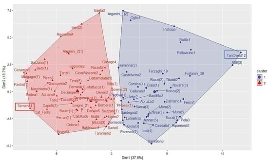
Figure 2.
Bi-dimensional plot of the two clusters obtained by k-means. Dimension 1 and 2 explain 37.8% and 13.7% of the variance, respectively. The rectangular frames highlight the two sites with the greatest distance (dissimilarity) between them in the bi-dimensional plot.
Figure 3 reports, for each cluster, the 24-h pattern of the hourly median values (thick lines) ± the median absolute deviation (MAD, grey area) for both δ and IR, as well as the observed time pattern (thin lines) for each of the sites included in the cluster. The patterns show that, in the night period (22:00–06:00), the IR values are the highest for both clusters because of the presence of noise events clearly emerging above the background noise, which is lower than that observed during the day-time. The hourly IR values for cluster 2 are higher than those for cluster 1 because the traffic flow for the sites belonging to cluster 2 is lower (mainly local roads) than that for the sites belonging to cluster 1. Figure 4 shows the straight comparison between the time patterns for the two clusters. The largest differences between the two clusters are observed during the night-time for δ and between 10:00 and 16:00 for IR. Thus, these periods are the most suitable to discriminate between the two clusters.
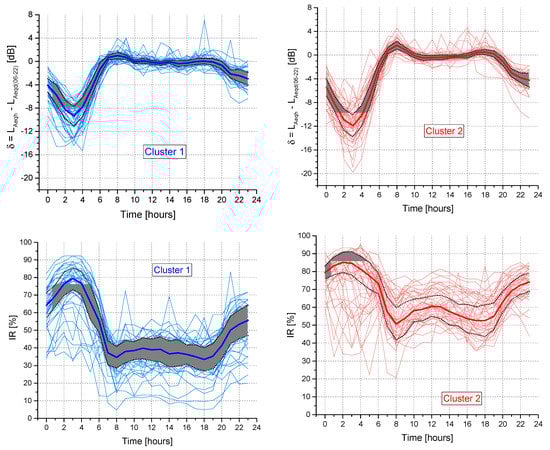
Figure 3.
Time patterns of δ and intermittency ratio (IR) parameters for the two clusters obtained by k-means (median values represented by thick lines and grey areas corresponding to ± median absolute deviation (MAD)) and actual values at each site (thin lines).
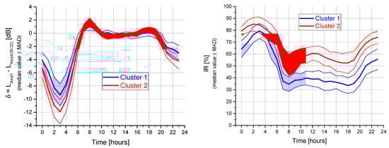
Figure 4.
Comparison of the time patterns of δ and IR parameters for the two clusters obtained by k-means. Thick lines represent hourly median values and shaded areas correspond to ± MAD.
3.2. Principal Component Analysis (PCA) Outcome
As explained in Section 2.2, PCA was performed in order to reduce the number of clustering variables. The scree plot, reported in Figure 5a for the first 12 components, shows that 10 components have eigenvalues ≥1, a value commonly used as a cutoff point at which principal components are retained. The cumulative percentage of variance explained by these 10 principal components is 86.7% (Figure 5b).
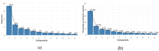
Figure 5.
Eigenvalues (a) and percentage of explained variance (b) for the first 12 principal components.
Thus, a matrix of 90 observations (the sites) and 10 variables, that is, the retained principal components (90/10 = 9), was the input for the k-means cluster analysis, setting the number of clusters to two. The obtained classification was completely in accordance with that already determined by k-means applied to the 48 variables. This result confirms the robustness of the partition obtained by k-means accounting for the 48 variables.
3.3. Comparison between Clustering Patterns of δ and IR Median Hourly Values and Measured Data
The rationale of determining the 24 h patterns of δ and IR for each cluster, shown in Figure 4, is to assign these patterns to the sites according to their cluster membership. This assignment, of course, introduces an uncertainty that should be evaluated (Figure 3). For this purpose, at each ith hour, the difference εi between the pattern cluster value (PCi) and the measured value (Mi) was determined:
εδi = δPCi − δMi [dB],
εIRi = IRPCi − IRMi [%],
This error ε can be expressed in different ways, either as relative error εr,
or as the root mean square of the error ε (RMSE),
where n is the number of observations (sites) in each cluster. Indeed, the patterns have their own uncertainties (grey areas in Figure 3), but, for sake of simplicity, only their median values are considered in the following.
εrIR = (IRPi − IRMi)/IRMi,
For practical application, the RMSE error in dB was considered for the δ parameter because it is more representative (Figure 6a), whereas for IR, measured in %, the relative error εr was chosen and is reported in Figure 6b. For all the sites belonging to the same cluster, the εi absolute values for each ith hour were determined and grouped (in %) in an interval bin width from 0.5 to 3 dB with steps of 0.5 dB. The median values of these percentages for each interval width were determined for the day (06:00–22:00) and night (22:00–06:00) periods and are plotted in Figure 6c,d, together with fitting curves. No large differences between clusters are observed for the error εδ determined for δ; the largest values of RMSE error (Figure 6a) and the lowest values of the percentage of εδ (Figure 6c) are observed for the period 00:00–05:00 (median error εδ > 2.0 dB), which, on the other hand, is the most suitable to discriminate between the two clusters. The relative error εrIR for IR is greater for cluster 1 during the day-time (06:00–22:00) (Figure 6b, median error εrIR = 0.63).
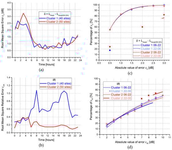
Figure 6.
Differences between the hourly values of the cluster patterns and the measured values in terms of root mean square (RMSE) (a,b) and percentage of error ε of being within an interval width (c,d).
3.4. Application of the δ and IR Cluster Patterns to New Data
To classify new roads according to the already determined clusters, it is necessary to find which cluster centroid is the closest to the new acoustic data. As an alternative, supervised machine-learning algorithms can be used and, among them, the k-nearest neighbors (k-NN) is the most common. Let us consider a road not included in the dataset used for determining the clusters (original data), with known δ and IR hourly values (new data). The k-NN algorithm searches for the k-nearest original data, in Euclidean distance, closer to the new data, and the classification is decided by majority vote. If there are ties for the kth nearest vector, all candidates are included in the vote.
Unfortunately, this procedure most often cannot be applied because the acoustic data for the road are unknown. Thus, it is necessary to look for an alternative classifier, hopefully linked to a specific feature of the road and/or to the corresponding traffic flow.
In noise monitoring surveys, to save time and reduce costs, stratified samplings of urban road traffic noise based on some attributes (i.e., road categorization) are commonly used. Their features and performances have been already analyzed, for instance, in [,]. Traffic flow (q), that is, the number of vehicles passing a point per unit of time (24 h, 1 h, and so on), can be a potential parameter for such a linkage because it represents information (observed or estimated by transport models) usually available for urban roads and used for their categorization in noise studies [].
In a previous paper [], the decimal logarithm of the day-time (06:00–22:00) total traffic flow, hereinafter “x”, has been proposed as a “non-acoustic” parameter to be applied to assign cluster membership. This choice was preferred to the 24-h traffic flow because of the observed large uncertainty of the night flow calculated by the traffic model []. Indeed, further investigations [,] have shown that there are significant differences between the traffic flow data provided by the model and those measured. This points to the need for more accurate data and, on this issue, there is an increasing interest to obtain real traffic flow data, for instance, through methodologies based on video processing and object detection tools [], or on travel time data obtained by Google Application Programming Interface (API) and Big Data treatment [].
Figure 7a shows the histograms of the data (bin width of x = 0.1) according to their cluster membership. It can be seen that, for 12 out of 26 bins (46.2%), there is an overlap between the two distributions. In order to figure out a threshold value to discriminate the cluster membership, the procedure to determine an analytical representation of the distribution functions in each cluster, as described in [,], was applied. The probability distributions for the two clusters P(x) can be obtained from the analytical fit of the cumulative distribution I(x) according to the following relationship:
where f(x) is a 3rd order polynomial, f’(x) is the derivative of f(x), and I(x) is the cumulative distributions of x. The fit functions and for obtained for the two clusters are as follows:
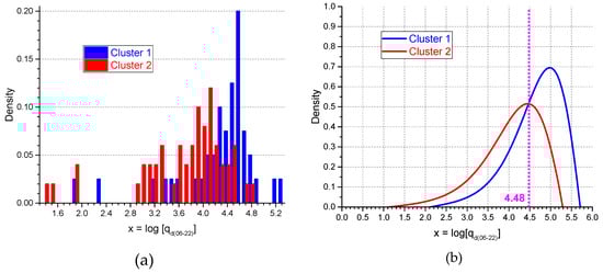
Figure 7.
Distributions of the data (bin width of x = 0.1) according to their cluster membership (a) and corresponding estimated probability distribution functions (b).
They are plotted in Figure 7b for the two distributions and show the “probability” that a road with a given “x” belongs to clusters 1 (blue curve) and 2 (red curve), respectively. It can be seen that, for x < 4.48 (intersection of the two curves), membership to cluster 2 can be roughly assumed, whereas for x ≥ 4.48, membership to cluster 1 seems to be more appropriate. The classification of sites based on this threshold value (roughly corresponding to an average hourly traffic flow of 1900 vehicles/hour) is in accordance with the original cluster memberships for 71.9% of the sites, a satisfactory value for the performance of the binary classifier “x”. In particular, on the basis of this threshold, the number of sites included in cluster 1 (high traffic flow) decreases from 40 (clustering partition) to 23 (classification by “x”) and, conversely, those included in cluster 2 (medium-low traffic flow) increase from 50 (clustering partition) to 67 (classification by “x”).
Table 3 reports the median values of RMSE relative error εr (Equation (7)) for δ and IR determined for the day and night periods and the two classifications based on clustering and the “non-acoustic” parameter x. The values in bold-italics point out the situations (4 out of 16) where the classification based on the binary classifier “x” is more accurate than that based on clustering. For the opposite situations, it has to be addressed that the classification based on “x” makes possible the association of new roads to the clusters also when acoustic data of them are unknown and only the day-time traffic flow is available.
Table 3.
Root mean square error (RMSE) median values of relative error εr for δ and IR determined for the day and night periods and the two classifications based on clustering and the “non-acoustic” parameter x.
4. Discussion
Road categorization is often applied to stratified samplings of urban road traffic noise based on some road attributes. This sampling, aimed to get data variability within each stratum less than that between the strata, can be fruitfully applied not only to optimize the resources and time involved in noise monitoring [], but also to be integrated in the noise mapping process []. Unfortunately, among the possible road attributes to be selected for categorization, the Italian road functional classification appears to not be appropriate because, as clearly shown in Table 2, the partitions determined by k-means cluster analysis include different road types. The k-means cluster analysis was also performed selecting site partitions into four groups to be numerically consistent with the four functional road categories. The comparison reported in Table 4 shows a large mismatch between the two approaches, namely 58.9% of the sites were differently grouped. This is most likely because of the inadequacy of functional road classification to represent the actual use and noise emission of roads.
Table 4.
Distribution of the 90 sites across type of road and four partitions obtained by k-means cluster analysis; percentage values are between ( ).
The data partition obtained by clustering (see Table 2) is satisfactory as the two clusters have similar size (40 and 50 sites) and are fairly separated. Cluster 1 includes sites with medium-high traffic flow, whereas cluster 2 is formed by sites with low-medium traffic flow (median value of the average day-time hourly traffic flow equal to 1760 and 470 vehicles/hour, respectively). As shown in Table 2, the obtained classification taking into account δ and IR is rather similar to that considering hourly IR values only, as they overlap for 93.3%. The misclassifications are observed only for road types “E” (four sites) and “F” (two sites).
It is interesting to point out that the major differences between the two clusters for both δ and IR are observed during the night period (22:00–06:00), as clearly shown in Figure 8. Thus, in the view of reducing the number of variables to be taken into account in the clustering process, those included in the night-time might represent potential candidates (16 variables instead of 48).
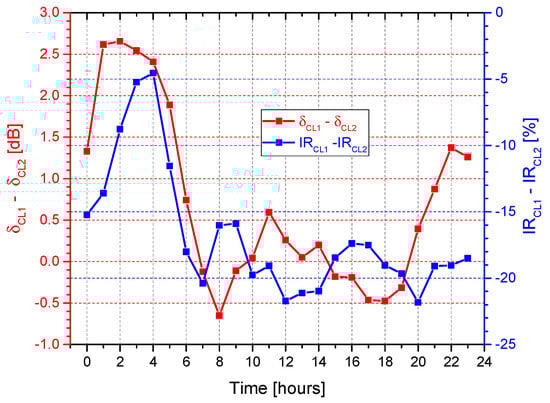
Figure 8.
Differences of the median value patterns of δ and IR between the two clusters (CL1 = cluster 1, CL2 = cluster 2).
To gain deeper insights of the differences between the two clusters, the farthest two sites in the cluster bi-plot in Figure 2 were selected (highlighted by rectangular frames in Figure 2), and each of the parameters reported in Table 5 and Figure 9 were examined. Table 5 reports, for each site, the hourly interval when the maximum value of the parameter was observed, whereas Figure 9 shows the density plots of the hourly values distribution. For the four parameters examined, their maximum values are observed within the period of 00:00–09:00. In particular, for LAeqh, the density distributions have a similar shape, whereas for IR, the maximum values are observed between the interval 02:00–04:00; the local road (cluster 2) shows a slightly higher number of events than the motorway (cluster 1). For the sound exposure level (SEL), the density distributions show similar modes, but that for cluster 1 is right-skewed and that for cluster 2 is left-skewed.
Table 5.
Maximum values of the parameters examined and corresponding hourly interval.
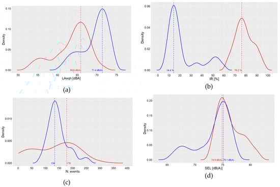
Figure 9.
Density plots of 24 hourly values of acoustic parameters LAeqh (a), IR (b), number of events (c), and sound exposure level (SEL) (d) for two sites belonging to different clusters (blue = cluster 1, red = cluster 2) and far away from each other in the cluster bi-plot (see Figure 2). Dotted lines show the mode of the density distributions.
Regarding the output of PCA, the correlation plot, showing the contributions of the variables in accounting for the variability in the two first principal components, is reported in Figure 10. It can be seen that dimension 1 can be interpreted as describing the eventfulness of the noise as the most contribution comes from the IR metric, whereas dimension 2 is linked to the noise energy, with LAeqh being the most contributing variables.
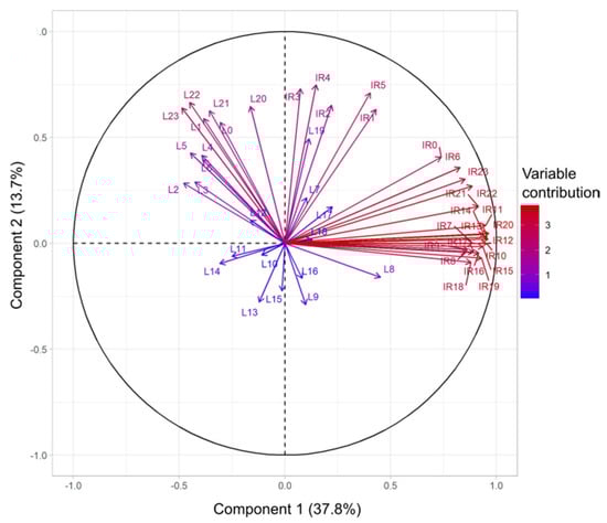
Figure 10.
Correlation plot of the principal component analysis (PCA). Component 1, describing 37.8% of the data variability, can be associated with the eventfulness of the noise (IR), whereas component 2, describing 13.7% of the data variability, can be associated with the noise energy (LAeq). L## stands for LAeqh and IR## for IRh.
To give an example of application of the above data classifications, let us consider three new roads for which the hourly values of δ and IR, dotted lines in Figure 11, as well as the non-acoustic parameter x, are known. According to the categorization based on x, because for all the three roads, the x value is less than 4.48, they should be classified into cluster 2, the centroid of which is also given in Figure 11, together with that of cluster 1. Running the k-NN algorithm with k = 1, all three roads are recognized to belong to cluster 2 as well. Thus, for these data, both classification criteria, based on clustering and the parameter x, agree in the cluster membership assignment.
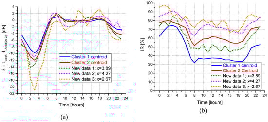
Figure 11.
Comparison of the new data roads, δ (a) and IR (b), with the centroids of the two clusters.
5. Conclusions
Cluster analysis was performed on a data sample of urban road traffic noise monitored in the city of Milan, formed by the hourly values of A-weighted continuous equivalent level LAeqh, describing the sound energy, and the intermittency ratio (IR), quantifying the noise events owing to vehicle pass-by.
The obtained two clusters can be fruitfully applied to stratify road sampling by choosing a representative road sample in each cluster and, therefore, to optimize noise monitoring resources []. The approach of road traffic noise clustering can be integrated in the noise mapping process too, as already applied in the DYNAMAP project [,], where a 24 h pattern representative of each cluster is assigned to non-monitored roads belonging to the cluster itself.
The assignment of new roads to the clusters can be obtained by supervised algorithms, like k-NN, when the acoustic data are known and, much more often, by a classifier linked to the road noise, herewith the logarithm of day-time (06:00–22:00) traffic flow. The two data partitions obtained by k-means clustering and by the threshold x = 4.48, corresponding to an average day-time hourly traffic flow of 1900 vehicles/hour, are in a satisfactory accordance (classification matching 71.9%).
Of course, the results are strongly dependent on the local situation and could not be generalized to other contexts. However, besides the above limitations, the described methodology could be fruitfully applied on road traffic noise data in other cities, allowing to compare different noise contexts.
Author Contributions
Conceptualization, G.B. and R.B.; methodology, G.B. and R.B.; software, G.B.; formal analysis, G.B.; investigation, G.B., R.B., and H.E.R.; data curation, C.C.; writing—original draft preparation, G.B.; writing—review and editing, R.B.; supervision, R.B. and G.Z.; funding acquisition, G.Z. All authors have read and agreed to the published version of the manuscript.
Funding
This research received no external funding.
Conflicts of Interest
The authors declare no conflict of interest.
References
- European Environment Agency. Noise in Europe 2014; EEA Report No 10/2014; Publications Office of the European Union: Luxembourg, 2014. [Google Scholar]
- Fritschi, L.; Brown, A.L.; Kim, R.; Schwela, D.H.; Kephalopoulos, S. (Eds.) Burden of Disease from Environmental Noise; World Health Organization: Bonn, Germany, 2011. [Google Scholar]
- Directive, E.U. Directive 2002/49/EC of the European Parliament and of the Council of 25 June 2002 relating to the assessment and management of environmental noise. Off. J. Eur. Communities L 2002, 189, 12–25. [Google Scholar]
- Can, A.; Aumond, P.; Michel, S.; de Coensel, B.; Ribeiro, C.; Botteldooren, D.; Lavandier, C. Comparison of noise indicators in an urban context. In Proceedings of the InterNoise 2016, Hamburg, Germany, 21–24 August 2016; pp. 5678–5686. [Google Scholar]
- De Coensel, B.; Botteldooren, D.; De Muer, T.; Berglund, B.; Nilsson, M.E.; Lercher, P. A model for the perception of environmental sound based on notice-events. J. Acoust. Soc. Am. 2009, 126, 656–665. [Google Scholar] [CrossRef] [PubMed]
- Bockstael, A.; De Coensel, B.; Lercher, P.; Botteldooren, D. Influence of temporal structure of the sonic environment on annoyance. In Proceedings of the 10th International Congress on Noise as a Public Health Problem (ICBEN), London, UK, 24–28 July 2011; pp. 945–952. [Google Scholar]
- Wunderli, J.M.; Pieren, R.; Habermacher, M.; Vienneau, D.; Cajochen, C.; Probst-Hensch, N.; Röösli, M.; Brink, M. Intermittency ratio: A metric reflecting short-term temporal variations of transportation noise exposure. J. Expo. Sci. Environ. Epidemiol. 2015, 26, 575–585. [Google Scholar] [CrossRef] [PubMed]
- Brambilla, G.; Confalonieri, C.; Benocci, R. Application of the Intermittency Ratio Metric for the Classification of Urban Sites Based on Road Traffic Noise Events. Sensors 2019, 19, 5136. [Google Scholar] [CrossRef]
- Zambon, G.; Angelini, F.; Salvi, D.; Zanaboni, W.; Smiraglia, M. Traffic noise monitoring in the city of Milan: Construction of a representative statistical collection of acoustic trends. In Proceedings of the ICSV22, Florence, Italy, 12–16 July 2015. [Google Scholar]
- R Core Team R: A Language and Environment for Statistical Computing; R Foundation for Statistical Computing: Vienna, Austria, 2018. Available online: https://www.R-project.org/ (accessed on 22 January 2020).
- Zambon, G.; Benocci, R.; Brambilla, G. Statistical Road Classification Applied to Stratified Spatial Sampling of Road Traffic Noise in Urban Areas. Int. J. Environ. Res. 2016, 10, 411–420. [Google Scholar]
- Wunderli, J.M.; Pieren, R.; Vienneau, D.; Cajochen, C.; Probst-Hensch, N.; Röösli, M.; Brink, M. Parameter study on IR, a metric reflecting short-term temporal variations of transportation noise exposure. In Proceedings of the 45th INTERNOISE, Hamburg, Germany, 21–24 August 2016; pp. 5710–5719. [Google Scholar]
- Brock, G.; Pihur, V.; Datta, S.; Datta, S. clValid: An R Package for Cluster Validation. J. Stat. Softw. 2008, 25, 1–22. [Google Scholar] [CrossRef]
- Murtagh, F.; Legendre, P. Ward’s Hierarchical Clustering Method: Clustering Criterion and Agglomerative Algorithm. J. Classif. 2014, 31, 274–295. [Google Scholar] [CrossRef]
- Kaufman, L.; Rousseeuw, P. Finding Groups in Data - An Introduction to Cluster Analysis; Wiley Series in Probability and Mathematical Statistics: New York, NY, USA, 1990. [Google Scholar]
- Hartigan, J.A.; Wong, M.A. A K-means clustering algorithm. Appl. Stat. 1979, 28, 100–108. [Google Scholar] [CrossRef]
- Yin, H. The Self-Organizing Maps: Background, Theories, Extensions and Applications. Stud. Comput. Intell. 2008, 115, 715–762. [Google Scholar]
- Dopazo, J.; Carazo, J.M. Phylogenetic reconstruction using a growing neural network that adopts the topology of a phylogenetic tree. J. Mol. Evol. 1997, 44, 226–233. [Google Scholar] [CrossRef]
- Fraley, C.; Raftery, A.E. Model-based clustering, discriminant analysis, and density estimation. J. Am. Stat. Assoc. 2002, 97, 611–631. [Google Scholar] [CrossRef]
- Dunn, J.C. A Fuzzy Relative of the ISODATA Process and Its Use in Detecting Compact Well-Separated Clusters. J. Cybern. 1973, 3, 32–57. [Google Scholar] [CrossRef]
- Halkidi, M.; Batistakis, Y.; Vazirgiannis, M. On Clustering Validation Techniques. J. Intell. Inf. Syst. 2001, 17, 107–145. [Google Scholar] [CrossRef]
- Liu, Y.; Li, Z.; Xiong, H.; Gao, X.; Wu, J. Understanding of Internal Clustering Validation Measures. In Proceedings of the IEEE International Conference on Data Mining, Sydney, Australia, 13 December 2010; pp. 911–916. [Google Scholar]
- Handl, J.; Knowles, J.; Kell, D.B. Computational Cluster Validation in Post-Genomic Data Analysis. Bioinformatics 2005, 21, 3201–3212. [Google Scholar] [CrossRef]
- Rousseeuw, P.J. Silhouettes: A Graphical Aid to the Interpretation and Validation of Cluster Analysis. J. Comput. Appl. Math. 1987, 20, 53–65. [Google Scholar] [CrossRef]
- Dunn, J.C. Well Separated Clusters and Fuzzy Partitions. J. Cybern. 1974, 4, 95–104. [Google Scholar] [CrossRef]
- Datta, S.; Datta, S. Comparisons and Validation of Statistical Clustering Techniques for Microarray Gene Expression Data. Bioinformatics 2003, 19, 459–466. [Google Scholar] [CrossRef]
- Yeung, K.Y.; Haynor, D.R.; Ruzzo, W.L. Validating Clustering for Gene Expression Data. Bioinformatics 2001, 17, 309–318. [Google Scholar] [CrossRef]
- Pihur, V.; Datta, S.; Datta, S. Weighted rank aggregation of cluster validation measures: A Monte Carlo cross-entropy approach. Bioinformatics 2007, 23, 1607–1615. [Google Scholar] [CrossRef]
- Barrigón Morillas, J.M.; Gomez, V.; Mendez, J.; Vilchez, R.; Trujillo, J. A categorization method applied to the study of urban road traffic noise. J. Acoust. Soc. Am. 2005, 117, 2844–2852. [Google Scholar] [CrossRef]
- Carmona del Río, F.J.; Escobar, V.G.; Carmona, J.T.; Vílchez-Gómez, R.; Méndez Sierra, J.A.; Rey Gozalo, G.; Barrigón Morillas, J.M. A Street Categorization Method to Study Urban Noise: The Valladolid (Spain) Study. Environ. Eng. Sci. 2011, 28, 811–817. [Google Scholar] [CrossRef]
- Escobar, V.G.; Pérez, C.J. An objective method of street classification for noise studies. Appl. Acoust. 2018, 141, 162–168. [Google Scholar] [CrossRef]
- Zambon, G.; Benocci, R.; Bisceglie, R.; Roman, H.E.; Bellucci, P. The LIFE DYNAMAP project: Towards a procedure for dynamic noise mapping in urban areas. Appl. Acoust. 2017, 124, 52–60. [Google Scholar] [CrossRef]
- Benocci, R.; Confalonieri, C.; Roman, H.R.; Angelini, F.; Zambon, G. Accuracy of the Dynamic Acoustic Map in a Large City Generated by Fixed Monitoring Units. Sensors 2020, 20, 412. [Google Scholar] [CrossRef]
- Benocci, R.; Molteni, A.; Cambiaghi, M.; Angelini, F.; Roman, H.E.; Zambon, G. Reliability of DYNAMAP traffic noise prediction. Appl. Acoust. 2019, 156, 142–150. [Google Scholar] [CrossRef]
- Guarnaccia, C. EAgLE: Equivalent Acoustic Level Estimator Proposal. Sensors 2020, 20, 701. [Google Scholar] [CrossRef]
- Licitra, G.; Moro, A.; Teti, L.; Del Pizzo, A.; Bianco, F. A new approach using big data to improve road traffic noise mapping. In Proceedings of the ICA 2019, Aachen, Germany, 9–13 September 2019; pp. 5167–5173. [Google Scholar]
- Zambon, G.; Benocci, R.; Brambilla, G. Cluster categorization of urban roads to optimize their noise monitoring. Environ. Monit. Assess. 2016, 188, 26. [Google Scholar] [CrossRef]
- Benocci, R.; Angelini, F.; Cambiaghi, M.; Bisceglie, A.; Roman, H.E.; Zambon, G.; Alsina-Pagès, R.M.; Socoró, J.C.; Alías, F.; Orga, F. Preliminary results of Dynamap noise mapping operations. In Proceedings of the INTER-NOISE 2018, Chicago, IL, USA, 26–29 August 2018. [Google Scholar]
- Zambon, G.; Roman, H.E.; Smiraglia, M.; Benocci, R. Monitoring and Prediction of Traffic Noise in Large Urban Areas. Appl. Sci. 2018, 8, 251. [Google Scholar] [CrossRef]
- Orga, F.; Socoró, J.C.; Alías, F.; Alsina-Pagès, R.M.; Zambon, G.; Benocci, R.; Bisceglie, A. Anomalous noise events considerations for the computation of road traffic noise levels: The DYNAMAP’s Milan case study. In Proceedings of the ICSV 2017, London, UK, 23–27 July 2017. [Google Scholar]
- Life-Dynamap. Available online: http://www.life-dynamap.eu/ (accessed on 2 April 2020).
© 2020 by the authors. Licensee MDPI, Basel, Switzerland. This article is an open access article distributed under the terms and conditions of the Creative Commons Attribution (CC BY) license (http://creativecommons.org/licenses/by/4.0/).