Experimental Investigation of Linear Encoder’s Subdivisional Errors under Different Scanning Speeds

Featured Application

The methodology described in the manuscript could be useful in a field of industrial automation for subdivisional linear-encoder error estimation and the improvement of final application performance in which the tested encoder is used.

Abstract

Optical encoders are widely used in applications requiring precise displacement measurement and fluent motion control. To reach high positioning accuracy and repeatability, and to create a more stable speed-control loop, essential attention must be directed to the subdivisional error (SDE) of the used encoder. This error influences the interpolation process and restricts the ability to achieve a high resolution. The SDE could be caused by various factors, such as the particular design of the reading head and the optical scanning principle, quality of the measuring scale, any kind of relative orientation changes between the optical components caused by mechanical vibrations or deformations, or scanning speed. If the distorted analog signals are not corrected before interpolation, it is very important to know the limitations of the used encoder. The methodology described in this paper could be used to determine the magnitude of an SDE and its trend. This method is based on a constant-speed test and does not require high-accuracy reference. The performed experimental investigation of the standard optical linear encoder SDE under different scanning speeds revealed the linear relationship between the tested encoder’s traversing velocity and the error value. A more detailed investigation of the obtained results was done on the basis of fast Fourier transformation (FFT) to understand the physical nature of the SDE, and to consider how to improve the performance of the encoder.

1. Introduction

Optical encoders are usually the most reliable devices for precise displacement measurement and motion control. Due to their high accuracy, resolution, and repeatability, as well as their ability to work under different environmental conditions and their relatively low price, they are used in a variety of applications. Some examples are manually controlled machine tools and computer-numerical-control (CNC) machines [1,2,3,4], robotics [5,6,7,8,9,10], servosystems [11,12,13,14], monitoring and fault diagnosis systems [15,16,17,18], tracking systems [19,20], linear and rotary positioning stages [21,22,23,24], and other precision-positioning applications [25].

The overall accuracy and precision of the linear encoder mainly depend on the quality of the measuring scale graduation and nonlinear subdivisional error (SDE) in one signal period [26]. Standard photoelectric linear encoders typically have a measuring scale with a period of 20 or 40 µm [27,28]. In order to increase resolution, two analog electric signals generated by an encoder are converted to digital and interpolated [29,30]. The smallest increment that can be detected may then reach the nanometer level. High accuracy and resolution are very important for applications that require precise positioning and good repeatability. In some applications, a linear encoder is used not only for position estimation, but also to provide feedback for speed control. A higher resolution ensures more stable and accurate position and speed loop.

The SDE (also called the interpolation error) is a cyclic error that repeats with each period of encoder grating. It depends on the quality of a main measuring scale and of the generated electric signals. This error appears during the interpolation process because the encoder’s distorted analog electric signals prevent the formation of a fine quadrature signal. In practice, the SDE does not cause any issues until its magnitude reaches the size of a measuring step. In other words, the magnitude of the SDE is a limit for the highest resolution. The minimal measurable incremental step has no point if the position error is greater. It is particularly important for applications requiring precise positioning and repeatability. In machines of which the feed axes or rotation tables are direct-driven, these nonlinear interpolation errors can cause not only positioning inaccuracies, but also result in loud noise, additional heat generation, and speed ripple [31].

The quality of the electrical signals highly depends on various aspects, like the optical-scanning principle, the design of a reading head and its ability to handle various deformations [32], mechanical vibrations [33,34,35], or temperature variations [36,37]. In order to improve signal quality and to make encoders more robust, manufacturers use advanced optical-scanning methods such as the single-field or interferential scanning principle [38,39], or they implement special-configuration multiple-track analyzer grating to eliminate higher-order harmonic signals [40]. Unfortunately, all such improvements require more complex encoder configurations and expensive optical parts. Another way to minimize SDE is electronic-signal correction. Nonideal signal parameters, such as relative amplitude, DC offset, phase shift, and nonsinusoidal shape, must be corrected before the interpolation process. Many studies dealt with this problem by using digital filtering and look-up tables, or by creating different algorithms for offline and dynamic compensation [41,42,43,44,45]. Because SDE is a short-range error that repeats each period, its compensation is a hard task.

It is very important to know the actual limits of the used displacement-measurement encoder so that the application can work smoothly and be properly tuned. SDE is one of the parameters that should be investigated first, especially if the electrical signals of the encoder are not corrected or compensated before an interpolation process. The methodology presented in this paper allows the estimation of interpolation-error magnitude and its trend across one period. The performed experimental investigation of the particular standard linear encoder interpolation error under different scanning speeds showed that the magnitude of this low-frequency error highly depends on the traversing speed of the encoder’s reading head. Moreover, a detailed harmonic analysis of the SDE could help to understand the physical nature of the error, and improve the performance of the encoder and the whole application.

2. Metrological Process and Subdivisional Errors in Optical Encoders

Optical linear encoders use various types of optical-scanning principles (e.g., Talbot effect [46,47], Lau effect [48,49], Moiré effect [50,51,52], generalized grating imaging [53,54,55,56], interferometric [57,58,59]) to generate electric-output signals that are used to determine a precise position. Depending on subsequently used electronics, optical encoders can have different interfaces to ensure the reliable exchange of information [60]. One of the most widely used interfaces for incremental position measurement is two analog nearly sinusoidal voltage signals (Figure 1). Signals A and B are shifted by 90 electrical degrees and have an amplitude of typically 1 Vpp. One full period (360 electrical degrees) of these signals corresponds to a period of grating on the measuring scale. Using the arctangent algorithm, it is easy to determine the relative position inside the period:

$$Xposition=\frac{p}{2\pi }arctan\left(\frac{S_A}{S_B}\right),$$

(1)

where $Xposition$, relative position between measuring scale and reading head; $p$, the period of the main scale; and $S_A,S_B$, values of output signals A and B in a certain position, respectively.

Such a process is known as interpolation, and it is directly related to the quality of the signals. The 1 Vpp interface is mainly used in applications where such an interpolation and analog-signal digitalization processes are executed by the subsequent electronics of the end-user equipment.

Combining analog encoder signals into the X and Y axes of an oscilloscope, it is comfortable to observe and follow the quality and accuracy of the encoder. The ideal signals give a perfectly centered circular shape with a diameter corresponding to signal amplitude. Unfortunately, in real applications, encoder output signals are distorted due to imperfections in manufacturing, and assembly and optical-scanning operations, as well as negatively affected by variations of environmental conditions. Distortion of the signals causes SDE, which repeats in each period of the encoder grating. Variations of the signal background level (U_{A_off}, U_{B_off}) are usually caused by imperfections or contaminants of the encoder measuring scale. Different signal offsets could also be related to the improper adjustment of electronic parts. Such a distortion leads to a decentered Lissajous curve, as shown in Figure 2a. Different peak-to-peak amplitudes (U_A, U_B) of the A and B signals could appear due to uneven or inconsistent illumination of the photodetectors. This error leads to an elliptical Lissajous curve, as shown in Figure 2b. A phase shift from 90 electrical degrees made the curve oval, as shown in Figure 2c. The main reason for this type of error is the tilt between the gratings of the scanning reticle and the main measuring scale. All higher harmonics caused by optical effects and electronics make signals that are not perfectly sinusoidal. This type of error forms a noncircular Lissajous curve, as shown in Figure 2d.

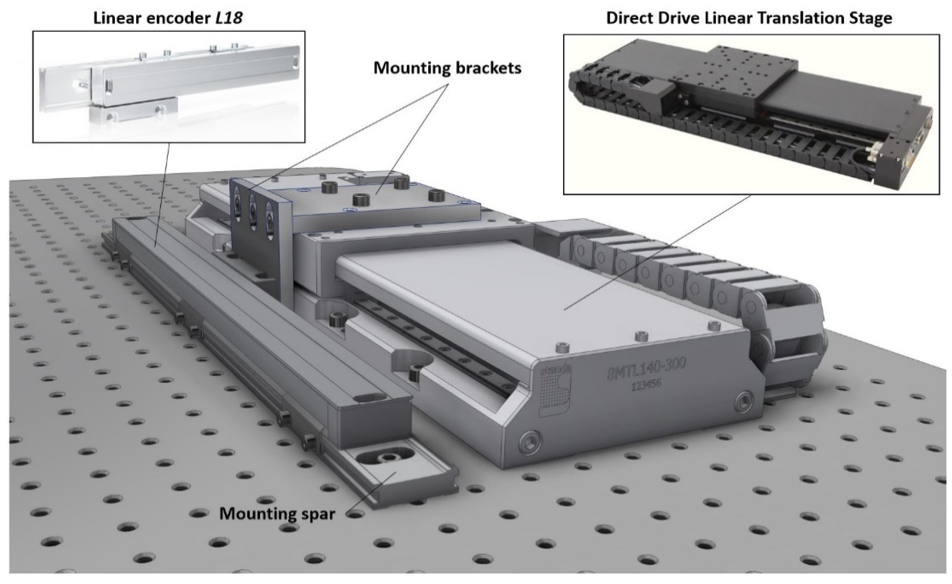
3. Investigation Methodology and Experiment Setup

The magnitude of an SDE is usually determined by using a reference encoder or a laser interferometer. Independent position information from a reference device is compared with a tested linear encoder reading, and the difference between these measures is accepted as the error. In order to perform such a test, a high-accuracy reference is needed.

Another method that was realized in this paper is based on a constant-speed test. The tested encoder reading head was driven at constant speed, and its electric-output signals were recorded using a digital oscilloscope. Because of high sampling frequency, analog encoder signals were represented as a group of discrete points. The relative position values inside one grating period could be calculated by putting these discrete points of A and B signals into Equation (1). Claiming that scanning speed is constant, and knowing the used sampling rate that must be selected by taking into account the Nyquist–Shannon sampling theorem and the acceptable size of the sample, it is easy to compose the theoretically true position values at these points. For example, if the scanning speed is 100 mm/s, the grating period of the tested encoder is 20 µm, and the sampling frequency is 250 MHz, there are 50,000 sampling points per one period. The first point corresponds to a zero position value, and the last one (50,000) corresponds to 20 µm. All other points increase with a step of 0.0004 µm. Then, the calculated values according to the arctangent algorithm could be compared with theoretically determined “true” position values. The differences are accepted as metrological linear encoder errors inside one grating period. In order to obtain statistically reliable results, this procedure must be repeated for several periods or several separate measurements, and the average value must be used. The accuracy of this methodology highly depends on the instability of the scanning speed and the precision of the used equipment. However, this method is completely suitable to determine the magnitude level of the error and to notice its trend.

A standard optical (4-field scanning) linear encoder was selected for this experimental investigation. The special technological setup was designed to determine its metrological errors under different scanning speeds. A motorized translation stage based on direct-drive technology was used to drive-test the encoder’s reading head at various constant speeds with high accuracy and low friction. The designed setup is shown in Figure 3.

The 3-phase ironless linear brushless servo motor of the translation stage was controlled by an ACS servo motion controller with a built-in driver. In the translation stage, an integrated noncontact linear optical encoder was used as a feedback system for high-resolution positioning and fluent motion control. Electric signals were sampled and recorded by using a digital oscilloscope. Schematic representation of the experiment setup is shown in Figure 4.

Experiment setup consisted of:

• Motion controller: servo motion controller with a built-in driver ACS Motion Control SPiiPlusCMnt.
• Linear-translation stage: motorized direct drive linear translation stage “STANDA” 8MTL1401-300.
• Tested linear encoder: optical (4-field scanning) linear encoder Precizika Metrology L18 (measuring length = 300 mm, grating period = 20 µm).
• Data acquisition and processing equipment. digital oscilloscope PicoScope 3000 and notebook with appropriate software.

Collected data were processed with computer software MATLAB. Determined SDE dependency on different scanning speeds was statistically evaluated by using a linear-regression approach. In order to analyze the nature of these errors at each speed, a fast Fourier transformation (FFT) algorithm was used. Because these errors are cyclic, their harmonic analysis helps to define what kind of signal imperfections cause them. The first harmonic of the SDE is a result of a nonzero background level of the A and B signals. The second harmonic could be caused by unequal amplitudes or a phase shift. Third and higher harmonics are the result of high-order distortions of the electric signals. Usually, they are caused by diffractive effects in optical-light modulation processes. Thus, an error decomposed into harmonics can be mathematically expressed by the following formula:

$$\delta \left(x\right)={{\displaystyle \sum }}_{i=1}^n{\displaystyle (}{A}_{i}cos(\frac{2\pi }{p}ix+{\phi }_i){\displaystyle )}+{\epsilon }_{n}for0\le x\le p,$$

(2)

where $\delta \left(x\right)$ denotes the SDE inside one period of the encoder grating, $A_i$ and ${\phi }_i$ indicate the amplitude and the phase of the harmonic, and $x$ denotes the relative position inside a period $p$. The number of the harmonic is marked as $n$, and $\epsilon$ indicates the random error.

4. Results and Discussion

First, performance of the tested linear encoder was checked under different scanning speeds. The maximal traversing velocity specified by a vendor of the encoder was 1 m/s. The Lissajous curves of several signal periods at 100, 500, and 1000 mm/s are shown in Figure 5.

From these graphs, it is clear that encoder performance started to differ when scanning speed was increased. The Lissajous curve changed its size and shape. Higher SDE was introduced. Moreover, several tested signal periods slightly varied from one another. This added additional uncertainty that had to be evaluated. For a more detailed investigation, the reading head of the tested encoder was driven at traversing velocities from 100 to 1100 mm/s with a step of 100 mm/s. The output electric signals were recorded by using a sampling frequency of 250 MHz, and the SDE was determined according to the methodology described in a previous section. Six different signal periods were randomly chosen to calculate the average value of the SDE at each speed level. As an example, the graphical representation of the electric signals and their combination in the X–Y plot when the reading head was driven at 300 mm/s is shown in Figure 6.

Calculated average SDE at this speed is shown in Figure 7. FFT analysis showed that the first, second, and third harmonics had the greatest influence on the error amplitude. Therefore, all three first harmonics are shown in the same graph to present the impact of each. The total magnitude of the error was ±0.185 µm. The second harmonic, which was repeated twice per period, created the biggest error value.

Similar data processing was made for all tested speeds. Calculated total error values were plotted into one graph, as shown in Figure 8. Results showed a strong linear relationship between scanning speed and total SDE. More than 85% of the experimentally determined error values could be mathematically associated with the increasing traversing speed of the encoder (R-squared = 0.8581). The low p-value confirmed that the applied linear-regression model was statistically significant (p-value = 0.00004 < 0.05). The biggest error was ±0.52 µm at 1100 mm/s. Two magnitudes at 900 and 1000 mm/s were quite distinct and distinguished from the linear relation.

To understand the physical meaning of the error that occurs during the scanning process, the magnitude and behavior of the first three error harmonics were analyzed. Their dependency on the tested encoder’s scanning speed is shown in Figure 9.

The biggest part of the SDE at each speed was caused by the second harmonic. This harmonic demonstrates a strong linear relationship (R-square = 0.96) to traversing velocity. Its size proportionally increased with increasing speed. This kind of error behavior is a result of signal-amplitude variation, phase shift, or their combination.

The first harmonic of the error demonstrates a nonlinear relationship. Amplitude values started to increase when the encoder reached a speed above 500 mm/s. An extreme jump of values was noticed in the range of 900–1000 mm/s. In this region, magnitude relatively dropped from 0.26 to 0.01 µm. This harmonic is a result of the emerged electric signals offset from a zero level.

The variation of the third harmonic meaning was not large in comparison with others. Its amplitude reached the highest value of 0.06 µm. This magnitude was noticed at a scanning speed of 900 mm/s, as with the first harmonic. Usually, this third harmonic is a result of variation in the optical-scanning process.

The following conclusions could be drawn from the obtained results:

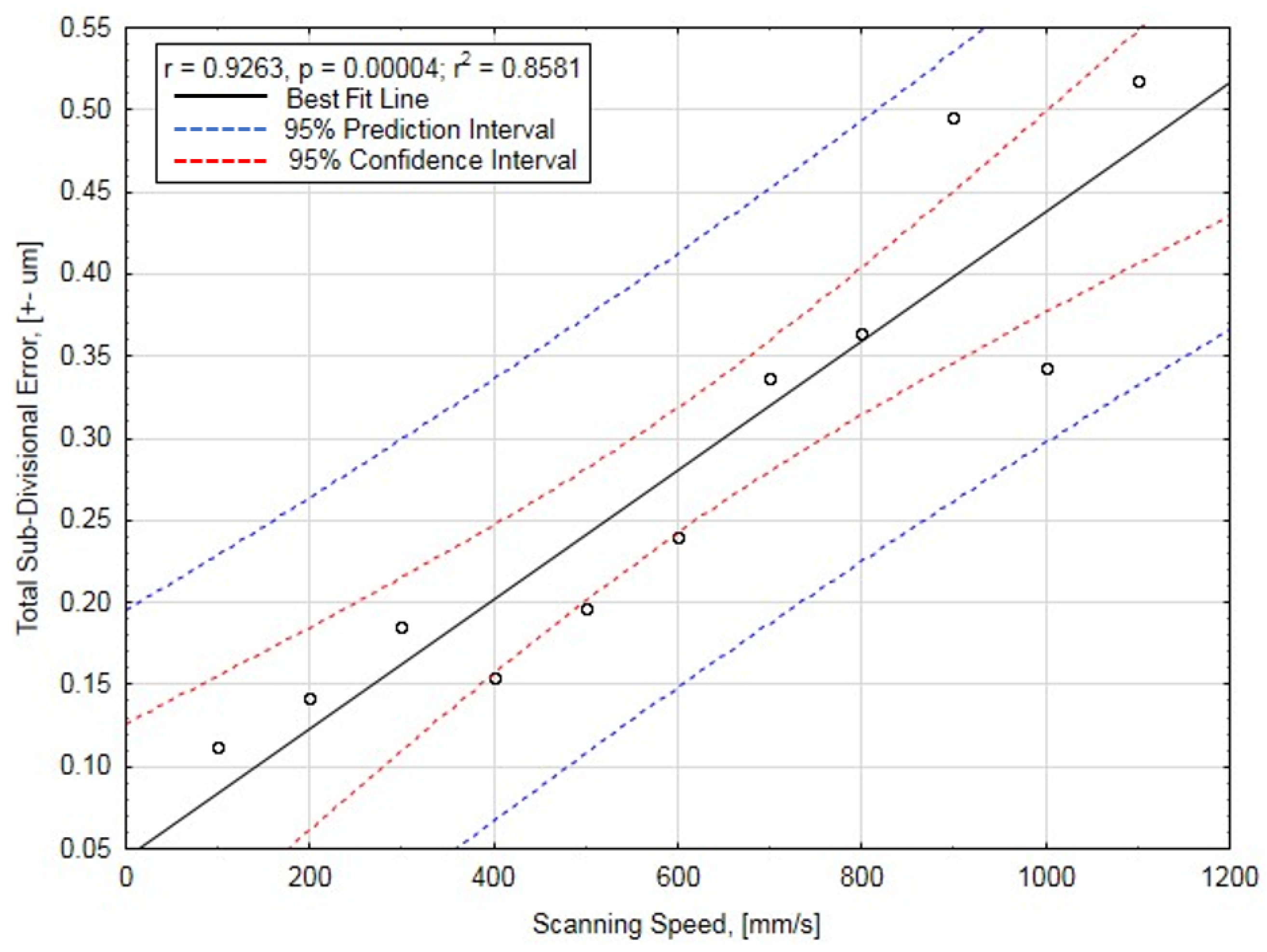
• The initial overview of the Lissajous curves showed that the SDE of the tested encoder depended on the scanning speed. More detailed analysis at different velocities is necessary to figure out the dependency.
• Statistical investigation showed a strong linear relationship between SDE and scanning speed. In this case, it is important to know the maximal traversing velocity at which the encoder runs in a specific application. Different maximal speed gives a different maximal SDE value and sets a distinct limitation for the highest resolution. In another case, when the SDE retains the same meaning in the whole speed range, or its relationship is nonlinear, the maximal SDE value should be determined.
• The maximal recommended traversing velocity of the encoder was 1 m/s. Working in this range, maximal SDE was ±0.49 µm, reached at 900 mm/s. After interpolation of these encoder signals, the resolution should be more than 0.5 µm. Otherwise, the interpolation error is bigger than the measuring step.
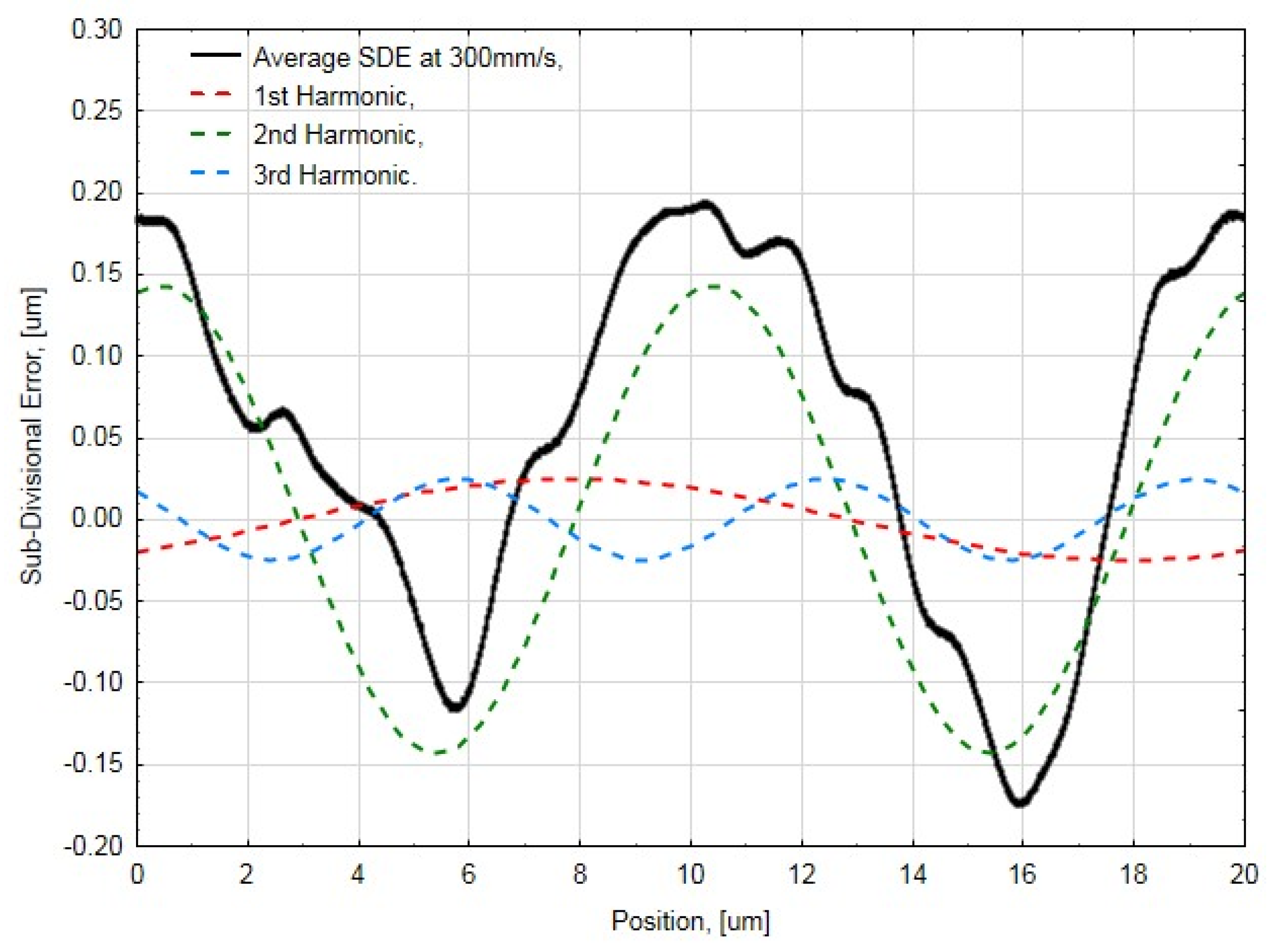
• At each speed, the biggest part of the SDE budget formed the second harmonic. This directly correlates to increasing velocity. This means that the difference of the signal amplitudes or the phase shift increased with speed. Amplitude, offset, or phase errors could be caused by the physics of the optical-scanning principle, and the dynamical behavior and improper adjustment of the electric components (like photodiodes, used processing chips, or analog amplifiers), or the quality of the used cable and other effects. It is necessary to pay attention to these aspects not only during the design process, but also while choosing a suitable encoder for a specific application. For example, the tested encoder’s working principle was based on the four-field scanning method. If the application requires more stability to scanning speed, or if there is an increased possibility of measuring scale contamination, the optical encoder based on the single-field scanning principle must be selected.
• The calculated total SDE values at 900 and 1000 mm/s velocities were distinct from the determined linear relationship. The magnitudes of the first and third harmonics reached their maximum values at 900 mm/s. When analyzing the first harmonic graph, in speeds above 500 mm/s the offset error of the encoder signals started to greatly vary. It is very likely that the dynamic behavior of the encoder was affected in this range of speed. The reading head is a complex mechanical part containing optical and electronic components, and flexible spring-based suspension, so even the smallest translation, distance variation, tilt, or other change in a relative position between scanning reticle and measuring scale could be generated by resonant frequency, friction, or other forces. For more detailed analysis, the generated frequencies at these speeds should be determined and compared with the natural frequencies of the encoder.
• FFT analysis showed that the major part of the SDE was made up of only a few first harmonics. That means that the trend of the SDE could be quite accurately approximated by using a simple equation that contains information of only the three first harmonics (n = 3).

  $$\delta \left(x\right)={\displaystyle \sum }_{i=1}^{n=3}{\displaystyle (}{A}_{i}cos(\frac{2\pi }{p}ix+{\phi }_i){\displaystyle )}for0\le x\le p$$

  (3)

After some extra processing of the experimental-investigation data, the multivariable function of the SDE value could be derived. This function could tell the approximated SDE value at a relative position inside the period at any scanning speed.

$$\delta \left(x,v\right)=f\left(x,v\right)+\epsilon ,for\{\begin{array}{c}0\le x\le p\\ 0<v\le v_{Max}\end{array};x,v\in Z,$$

(4)

where $f\left(x\right)$ is a multivariable approximation function of the SDE value, of which the arguments are relative position $x$ and scanning speed $v.$ $\epsilon$ indicates the random error, and $v_{Max}$ denotes the maximal traversing velocity of the encoder. This kind of equation could be used for real-time SDE compensation.

5. Conclusions

Linear encoders are often used in applications for the precise displacement measurement of a moving unit to control positioning and speed. In order to properly accomplish these tasks, encoder parameters such as accuracy and resolution are critical. In practice, a SDE in an optical encoder is unavoidable. The magnitude of this error is a major factor that limits maximal resolution and causes a speed ripple. When analog encoder signals are interpolated without any error correction or compensation approach, it is very important to know the limitations of the used encoder. The method described in this paper presents a way to determine the magnitude and trend of the linear encoder SDE.

Experimental investigation of the standard optical linear encoder SDE under different scanning speeds was accomplished according to the presented methodology. Deeper analysis of the determined errors helped to reveal their physical nature and the limits of the encoder. On the basis of the obtained results, it is possible to specify the weak points of the tested device to help to improve its performance. Mapped and approximated SDE at different speeds could be used as a multivariable function for positioning-error compensation. This is our future research direction.

References

1. Zhao, L.; Cheng, K.; Chen, S.; Ding, H.; Zhao, L. An approach to investigate moiré patterns of a reflective linear encoder with application to accuracy improvement of a machine tool. Proc. Inst. Mech. Eng. Part B J. Eng. Manuf. 2018, 233, 927–936. [Google Scholar] [CrossRef]
2. Bai, Q.; Liang, Y.; Cheng, K.; Long, F. Design and analysis of a novel large-aperture grating device and its experimental validation. Proc. Inst. Mech. Eng. Part B J. Eng. Manuf. 2013, 227, 1349–1359. [Google Scholar] [CrossRef]
3. Liu, C.; Jywe, W.; Hsu, T. The application of the double-readheads planar encoder system for error calibration of computer numerical control machine tools. Proc. Inst. Mech. Eng. Part B J. Eng. Manuf. 2004, 218, 1077–1089. [Google Scholar] [CrossRef]
4. Du, Z.; Zhang, S.; Hong, M. Development of a multi-step measuring method for motion accuracy of NC machine tools based on cross grid encoder. Int. J. Mach. Tools Manuf. 2010, 50, 270–280. [Google Scholar] [CrossRef]
5. Ishii, N.; Taniguchi, K.; Yamazaki, K.; Aoyama, H. Performance improvement of machine tool by high accuracy calibration of built-in rotary encoders. In Proceedings of the 9th International Conference on Leading Edge Manufacturing in 21st Century, Japan Society of Mechanical Engineers, Hiroshima, Japan, 13–17 November 2017. [Google Scholar]
6. Algburi, R.N.A.; Gao, H. Health assessment and fault detection system for an industrial robot using the rotary encoder signal. Energies 2019, 12, 2816. [Google Scholar] [CrossRef] [Green Version]
7. Han, Z.; Jianjun, Y.; Gao, L. External force estimation method for robotic manipulator based on double encoders of joints. In Proceedings of the IEEE International Conference on Robotics and Biomimetics (ROBIO), Kuala Lumpur, Malaysia, 12–15 December 2018. [Google Scholar]
8. Peng, L.; Xiangpeng, L. Common sensors in industrial robots: A review. J. Phys. Conf. Ser. 2019, 1267, 012036. [Google Scholar]
9. Mikhel, S.; Popov, D.; Mamedov, S.; Klimchik, A. Advancement of robots with double encoders for industrial and collaborative applications. In Proceedings of the 23th Conference of Open Innovations Association (FRUCT), Bologna, Italy, 13–16 November 2018. [Google Scholar]
10. Rodriguez-Donate, C.; Osornio-Rios, R.A.; Rivera-Guillen, J.R.; Romero-Troncoso, R.J. Fused smart sensor network for multi-axis forward kinematics estimation in industrial robots. Sensors 2011, 11, 4335–4357. [Google Scholar] [CrossRef] [Green Version]
11. Vazquez-Gutierrez, Y.; O’Sullivan, L.; Kavanagh, R.C. Study of the impact of the incremental optical encoder sensor on the dynamic performance of velocity servosystems. J. Eng. 2019, 2019, 3807–3811. [Google Scholar] [CrossRef]
12. Vazquez-Gutierrez, Y.; O’Sullivan, L.; Kavanagh, R.C. Small-signal modeling of the incremental optical encoder for motor control. IEEE Trans. Ind. Electron. 2019. [Google Scholar] [CrossRef]
13. Vazquez-Gutierrez, Y.; O’Sullivan, L.; Kavanagh, R.C. Evaluation of three optical-encoder-based speed estimation methods for motion control. J. Eng. 2019, 2019, 4069–4073. [Google Scholar] [CrossRef]
14. Zhang, Z.; Olgac, N. Zero magnitude tracking control for servo system with extremely low-resolution digital encoder. Int. J. Mechatron. Manuf. Syst. 2018, 10. [Google Scholar] [CrossRef]
15. Zhao, M.; Jia, X.; Lin, J.; Lei, Y.; Lee, J. Instantaneous speed jitter detection via encoder signal and its application for the of planetary gearbox. Mech. Syst. Signal Process. 2018, 98, 16–31. [Google Scholar] [CrossRef]
16. Li, B.; Zhang, X.; Wu, J. New procedure for gear fault detection and diagnosis instantaneous angular speed. Mech. Syst. Signal Process. 2017, 85, 415–428. [Google Scholar] [CrossRef]
17. Ariznavarreta-Fernandez, F.; Gonzalez-Palacio, C.; Menendez-Diaz, A.; Ordonez, C. Measurement system with angular encoders for continuous monitoring of tunnel convergence. Tunn. Undergr. Space Technol. 2016, 56, 176–185. [Google Scholar] [CrossRef]
18. Zhao, M.; Lin, J. Health assessment of rotating machinery using a rotary encoder. IEEE Trans. Ind. Electron. 2018, 65, 2548–2556. [Google Scholar] [CrossRef]
19. Tang, T.; Chen, S.; Huang, X.; Yang, T.; Qi, B. Combining load and motor encoders to compensate nonlinear disturbances for high precision tracking control of gear-driven Gimbal. Sensors 2018, 18, 754. [Google Scholar] [CrossRef] [PubMed] [Green Version]
20. Chong, K.K.; Wong, C.-W.; Siaw, F.-L.; Yew, T.-K.; Ng, S.-S.; Liang, M.-S.; Lim, Y.-S.; Lau, S.-L. Integration of an on-axis general sun-tracking formula in the algorithm of an open-loop sun-tracking system. Sensors 2009, 9, 7849–7865. [Google Scholar] [CrossRef] [PubMed] [Green Version]
21. Kimura, A.; Gao, W.; Kim, W.; Hosono, K.; Shimizu, Y.; Shi, L.; Zeng, L. A sub-nanometric three-axis surface encoder with short-period planar gratings for stage motion measurement. Precis. Eng. 2012, 36, 576–585. [Google Scholar] [CrossRef]
22. Lee, C.B.; Kim, G.H.; Lee, S.K. Design and construction of a single unit multi-function optical encoder for a six-degree-of-freedom motion error measurement in an ultraprecision linear stage. Meas. Sci. Technol. 2011, 22. [Google Scholar] [CrossRef]
23. Li, Y.T.; Fan, K.C. A novel method of angular positioning error analysis of rotary stages based on the Abbe principle. Proc. Inst. Mech. Eng. Part B J. Eng. Manuf. 2018, 232, 1885–1892. [Google Scholar] [CrossRef]
24. Lou, Z.F.; Hao, X.P.; Cai, Y.D.; Lu, T.F.; Wang, X.D.; Fan, K.C. An embedded sensors system for real-time detecting 5-DOF error motions of rotary stages. Sensors 2019, 19, 2855. [Google Scholar] [CrossRef] [PubMed] [Green Version]
25. Gao, W.; Kim, S.W.; Bosse, H.; Haitjema, H.; Chen, Y.L.; Lu, X.D.; Knapp, W.; Weckenmann, A.; Estler, W.T.; Kunzmann, H. Measurement technologies for precision positioning. CIRP Ann. Manuf. Technol. 2015, 64, 773–796. [Google Scholar] [CrossRef]
26. Smith, G.T. Machine Tool Metrology. An Industrial Handbook; Springer: Berlin, Germany, 2016; pp. 159–177. [Google Scholar]
27. Heidenhain. Linear Encoders for Numerically Controlled Machine Tools. Available online: https://www.heidenhain.com/fileadmin/pdb/media/img/571470-2C_Linear_Encoders_For_Numerically_Controlled_Machine_Tools.pdf (accessed on 22 January 2020).
28. Fagor Automation. Feedback Systems. Available online: https://www.fagorautomation.com/en/p/feedback-systems/ (accessed on 22 January 2020).
29. Ye, G.; Wu, Z.; Xu, Z.; Wang, Y.; Shi, Y.; Liu, H. Development of a digital interpolation module for high-resolution sinusoidal encoders. Sens. Actuators A Phys. 2019, 285, 501–510. [Google Scholar] [CrossRef]
30. Ye, G.; Liu, H.; Wang, Y.; Lei, B.; Shi, Y.; Yin, L.; Lu, B. Ratiometric-linearization -based high-precision electronic interpolator for sinusoidal optical encoders. IEEE Trans. Ind. Electron. 2018, 65, 8224–8231. [Google Scholar] [CrossRef]
31. Ye, G.; Xing, H.; Liu, H.; Li, Y.; Lei, B.; Niu, D.; Li, X.; Lu, B.; Liu, H. Total error compensation of non-ideal signal parameters for Moire encoders. Sens. Actuators 2019, 298. [Google Scholar] [CrossRef]
32. Alejandre, I.; Artes, M. Machine tool errors caused by optical linear encoders. J. Eng. Manuf. 2004, 218, 113–122. [Google Scholar] [CrossRef]
33. Lopez, J.; Artes, M.; Alejandre, I. Analysis of optical linear encoders errors under vibration at different mounting conditions. Measurement 2011, 44, 1367–1380. [Google Scholar] [CrossRef]
34. Lopez, J.; Artes, M.; Alejandre, I. Analysis under vibrations of optical linear encoders based on different scanning methods using an improved experimental approach. Exp. Tech. 2012, 36, 35–47. [Google Scholar] [CrossRef]
35. Lopez, J.; Artes, M. A new methodology for vibration error compensation of optical encoders. Sensors 2012, 12, 4918–4933. [Google Scholar] [CrossRef] [Green Version]
36. Alejandre, I.; Artes, M. Real thermal coefficient in optical linear encoders. Exp. Tech. 2004, 28, 18–22. [Google Scholar] [CrossRef]
37. Alejandre, I.; Artes, M. Thermal non-linear behaviour in optical linear encoders. Int. J. Mach. Tools Manuf. 2005, 46, 1319–1325. [Google Scholar] [CrossRef]
38. Rozman, J.; Pletersek, A. Linear optical encoder system with sinusoidal signal distortion below −60 dB. IEEE Trans. Instrum. Meas. 2010, 59, 1544–1549. [Google Scholar] [CrossRef]
39. Li, M.; Liang, Z.; Zhang, R.; Wu, Q.; Xin, C.; Jin, L.; Xie, K.; Zhao, H. Large-scale range diffraction grating displacement sensor based on polarization phase-shifting. Appl. Opt. 2020, 59, 469–473. [Google Scholar] [CrossRef]
40. Ye, G.; Liu, H.; Jiang, W.; Li, X.; Jiang, W.; Yu, H.; Shi, Y.; Yin, L.; Lu, B. Design and development of an optical encoder with sub-micron accuracy using a multiple-tracks analyser grating. Rev. Sci. Instrum. 2017, 88. [Google Scholar] [CrossRef]
41. Albrecht, C.; Klock, J.; Martens, O.; Schumacher, W. Online estimation and correction of systematic encoder line errors. Machines 2017, 5, 1. [Google Scholar] [CrossRef] [Green Version]
42. Mendenhall, M.H.; Windover, D.; Henins, A.; Cline, J.P. An algorithm for the compensation of short-period errors in optical encoders. Metrologia 2015, 52, 685. [Google Scholar] [CrossRef]
43. Ye, G.; Fan, S.; Liu, H.; Li, X.; Yu, H.; Shi, Y.; Yin, L.; Lu, B. Design of a precise and robust linearized converter for optical encoders using a ratiometric technique. Meas. Sci. Technol. 2014, 25. [Google Scholar] [CrossRef]
44. Yandayan, T.; Geckeler, R.D.; Just, A.; Krause, M.; Akgoz, S.A.; Aksulu, M.; Grubert, B.; Watanabe, T. Investigation of interpolation errors of angle encoders for high precision angle metrology. Meas. Sci. Technol. 2018, 29. [Google Scholar] [CrossRef]
45. Wang, Y.; Liu, Y.; Yan, X.; Chen, X.; Lv, H. Compensation of Moire fringe sinusoidal deviation in photoelectric encoder based on tunable filter. In Proceedings of the 2011 Symposium on Photonics and Optoelectronics (SOPO), Wuhan, China, 16–18 May 2011. [Google Scholar] [CrossRef]
46. Kao, C.F.; Huang, H.L.; Lu, H. Optical encoder based on Fractional-Talbot effect using two-dimensional phase grating. Opt. Commun. 2010, 283, 1950–1955. [Google Scholar] [CrossRef]
47. Kao, C.F.; Lu, H. Optical encoder based on the fractional Talbot effect. Opt. Commun. 2005, 250, 16–23. [Google Scholar] [CrossRef]
48. Crespo, D.; Alonso, J.; Tomas, M.; Eusebio, B. Optical encoder based on the Lau effect. Opt. Eng. 2000, 39, 817–822. [Google Scholar] [CrossRef]
49. Sudol, R.; Thompson, B.J. Lau effect: Theory and experiment. Appl. Opt. 1981, 20, 1107–1116. [Google Scholar] [CrossRef] [PubMed]
50. Li, X. Displacement measurement based on the Moire fringes. Int. Soc. Opt. Eng. 2011. [Google Scholar] [CrossRef]
51. Wu, J.; Zhou, T.T.; Yuan, B.; Wang, L.-Q. A digital Moire fringe method for displacement sensors. Front. Inform. Technol. Electron. Eng. 2016, 17, 946–953. [Google Scholar] [CrossRef]
52. Zhao, B.; Miao, J.; Xie, H.; Asundi, A. Modeling of grating/Moire based micro sensor. Microsyst. Technol. 2001, 7, 107–116. [Google Scholar] [CrossRef]
53. Ye, G.; Liu, H.; Xie, H.; Asundi, A. Optimizing design of an optical encoder based on generalized grating imaging. Meas. Sci. Technol. 2016, 27. [Google Scholar] [CrossRef]
54. Ye, G.; Liu, H.; Fan, S.; Li, X.; Yu, H.; Lei, B.; Shi, Y.; Yin, L.; Lu, B. A theoretical investigation of generalized grating imaging and its application to optical encoders. Opt. Commun. 2015, 354, 21–27. [Google Scholar] [CrossRef]
55. Liu, H.; Ye, G.; Shi, Y.; Yin, L.; Chen, B.; Lu, B. Multiple harmonics suppression for optical encoders based on generalized grating imaging. J. Mod. Opt. 2016, 63, 1564–1572. [Google Scholar] [CrossRef]
56. Iwata, K. Interpretation of generalized grating imaging. J. Opt. Soc. Am. 2008, 25, 2244–2250. [Google Scholar] [CrossRef]
57. Lee, C.-K.; Wu, C.-C.; Chen, S.-J.; Yu, L.-B.; Chang, Y.-C.; Wang, Y.-F.; Chen, J.-Y.; Wu, J.W.-J. Design and construction of linear laser encoders that possess high tolerance of mechanical run out. Appl. Opt. 2004, 43, 5754–5762. [Google Scholar] [CrossRef]
58. Liu, C.-H.; Jywe, W.-Y.; Wang, M.-S.; Huang, H.-L. Development of a three-degrees-of-freedom laser linear encoder for error measurement of a high precision range. Rev. Sci. Instrum. 2007, 78. [Google Scholar] [CrossRef]
59. Liu, C.H.; Cheng, C.H. Development of a multi-degree-of-freedom laser encoder using +- 1 order and +- 2 order diffraction rays. In Proceedings of the 10th International Symposium of Measurement Technology and Intelligent Instruments, Daejeon, Korea, 29 June–2 July 2011. [Google Scholar]
60. Heidenhain. Interfaces. Available online: https://www.heidenhain.com/en_US/documentation/fundamentals/interfaces/ (accessed on 22 February 2020).
Figure 1. Definition of differential optical encoder signals. 1 Vpp interface.
Applsci 10 01766 g001
Figure 2. Lissajous curves of optical-encoder signals with relative subdivisional error (SDE): (a) offset error; (b) amplitude error; (c) phase-shift error; (d) signal-shape error.
Applsci 10 01766 g002
Figure 3. Designed experiment setup. Tested linear encoder was connected to direct-drive linear translation stage through mounting bracket.
Applsci 10 01766 g003
Figure 4. Schematic view of experiment setup.
Applsci 10 01766 g004
Figure 5. Lissajous curves of several signal periods at different scanning speeds: 100, 500, and 1000 mm/s.
Applsci 10 01766 g005
Figure 6. Electric signals A and B and their representation in the X–Y plot. Encoder was working at 300 mm/s traversing velocity.
Applsci 10 01766 g006
Figure 7. Average SDE and its decomposition into three first harmonics when scanning speed is 300 mm/s.
Applsci 10 01766 g007
Figure 8. Total SDE dependency on scanning speed. Data points and their statistical parameters.
Applsci 10 01766 g008
Figure 9. Three first harmonics of determined SDEs at different scanning speeds.
Applsci 10 01766 g009