Investigation and Enhancement of the Detectability of Flaws with a Coarse Measuring Grid and Air Coupled Ultrasound for NDT of Panel Materials Using the Re-Radiation Method

Abstract

Non-destructive ultrasonic testing is utilized widely by industries for quality assurance. For sensitive materials or surfaces, non-contact, non-destructive testing methods are in demand. The air-coupled ultrasound (ACU) is one possible solution. This can be used to investigate large, panel-like objects for delaminations and other flaws. For a high detectability, fine measurement grids are required (typically <$\lambda$ is used), which results in extremely long data acquisition times that are only practicable for laboratory applications. This paper aimed at reducing the required measurement grid points for obtaining high detectability evaluations. The novel method presented in this paper allows a measurement grid that is much coarser than the resulting grid. The method combines a software refinement of the measured data with the Rayleigh–Sommerfeld diffraction integral for the calculation of the pressure distribution on the object’s surface. This result allows the precise prediction of delaminations and flaws in the tested object. The presented method shows a decrease in the total investigation time by up to 98%.

1. Introduction

Piezoelectric ultrasonic transducers have become indispensable in the field of non-destructive material testing, since Sokolov used continuous ultrasonic waves to identify material defects [1]. Those are usually used in a liquid medium due to the impedance matching of the transducer and the ambient medium. However, there are some materials that must not be immersed in a liquid, not even for testing. These include composite materials, like wood-based materials, that absorb the liquid and thus change its properties. Due to the acoustic impedance of an air/wood interface, only 0.1% of the initial energy can be transmitted [2]. However, powerful ultrasonic transducer and sensitive receiver were developed in recent years to address this [3]. Piezoelectric ultrasonic transducers can also be designed more easily if they do not require extra protection against liquids. So, for such kind of materials, air-coupled ultrasound (ACU) has established itself in many areas of non-destructive testing (NDT) after the high impedance difference between solid and gas could be overcome with new developments (e.g., application of a matching layer for impedance matching of piezoceramics to air) [4]. Wood products, in particular, are of great interest today and those cannot be tested in a liquid medium. The large, well-known furniture manufacturers want to be able to offer their furniture at ever lower prices. One step towards this is to make the particleboards used thinner and thinner. This saves material and money. However, they have to make sure that these pieces of furniture still withstand the loads. This is only possible if the suppliers can ensure that the particleboards are free of defects. Now, during the production process of a particleboard after gluing, pressing, and out gassing, air inclusions and imperfectly glued regions in the particleboard can strongly influence the load capacity [5]. Suppliers and/or manufacturers must, therefore, test their wood products non-destructively to meet the high demands of the furniture industry.

The use of NDT with ultrasound can be sorted into three groups: the pulse-echo technique, where flaws can be detected by the echo of a transmitted pulse wave and, with the known of the time of flight and the speed of sound in the test object, the depth of the flaw can be determined [6,7]; the surface-wave technique, where the surface near flaws can be detected, like the pulse-echo method, which is a one-side method, where the transmitter and the receiver is only at one side of the test object [8]; and the through-transmission technique, which is also used in this publication. In the through-transmission technique, the transmitter is at one side of the test object, and the receiver is at the opposite side [9,10]. This has the advantage compared to the pulse-echo technique in that the sound wave must transmit the test object only once; therefore, thicker material can be tested [3]. If the transmitter is stationary, and the receiver is moved in steps, tomographic measurements can be made. The transmitter emits a pulse-like sound wave via the coupling medium to the test object, where it is largely reflected and, to a small extent, transmitted. In the test object, the sound wave propagates until it reaches the next boundary of the test object to the ambient medium, where it is reflected and transmitted once more. The transmitted signal is recorded by receivers. Flaws in the material could change the impedance, consequently resulting in a decreased measurable pressure amplitude. The smaller acoustic pressure presents as a shadow in the pressure field and so can be detected.

These measurements can be transferred to different forms of visualization. The three best known are according to Döring [11]: an A-scan, which is only measured and evaluated at one point, where the time curve of the pressure or the sound amplitude at this position is evaluated; a B-scan, in which a line of measuring points is measured with an A-scan and with a defined distance, thus obtaining 2D information that can then be displayed either at a fixed time as a line graph or for a defined period of time as an area plot [12]; and a C-scan, which needs the highest effort because a surface that is discretized by a grid is measured one after the other, point by point, with single A-scans [13]. If the scanning plane is far away from the panel surface, then a volume scan can be done. At defined distances, planes are measured with a C-scan, and then those are combined to volumetric data to evaluate. This technique is very time-consuming [14]. Receiver arrays [15] can be used to shorten the measurement time, but such arrays have a great influence on the sound field. A detailed description of the common procedures of air-coupled ultrasound for the examination of wood materials can be found in Fang and Stößel [7,9].

However, in order to obtain the information of a volume sound field and to shorten the measuring time, one possibility is to measure only one plane in a C-scan and to calculate the volume sound field or the sound field of the air layer directly above the panel surface via post-processing methods. This can be done by the re-radiation method [16,17,18,19,20,21,22]. In this way, very well interpretable amplitude images of the air layer directly above the panel surface are generated. These allow the identification and localization of flaws or the heterogeneities in the materials [17,18,22]. To create a C-scan image with a high detectability of flaws by using a typical measurement grid with a grid point distance of $\le \frac{\lambda }{3}$ [16,17,18,22], many measurements have to be made, and this is comparatively time-consuming. Nevertheless, with the re-radiation method of Marhenke2019 [22] we were able to identify flaws which are smaller than $\lambda$. Therefore, there is a need for techniques that can be applied with the re-radiation method that provide high detectability of flaws in a C-scan image, while requiring less measurement time due to a coarser measurement grid $(>\frac{\lambda }{3})$.

In this publication, we propose a novel way of data post-processing before the use of the re-radiation method. This makes it possible to obtain images with a high detectability of flaws from a very coarse measuring grid (>$\lambda$) of a C-scan and to identify flaws which are smaller than $\lambda$. For this, the novel idea of virtual measuring grid points is used, which are filled with time data via different interpolation methods. This opens up the possibility of reducing the number of measuring grid points significantly, thus reducing the experiment time of up to 98%.

2. Materials and Methods

Section 2.1 describes the experimental setup, and Section 2.2 explains the mathematical theories that were used.

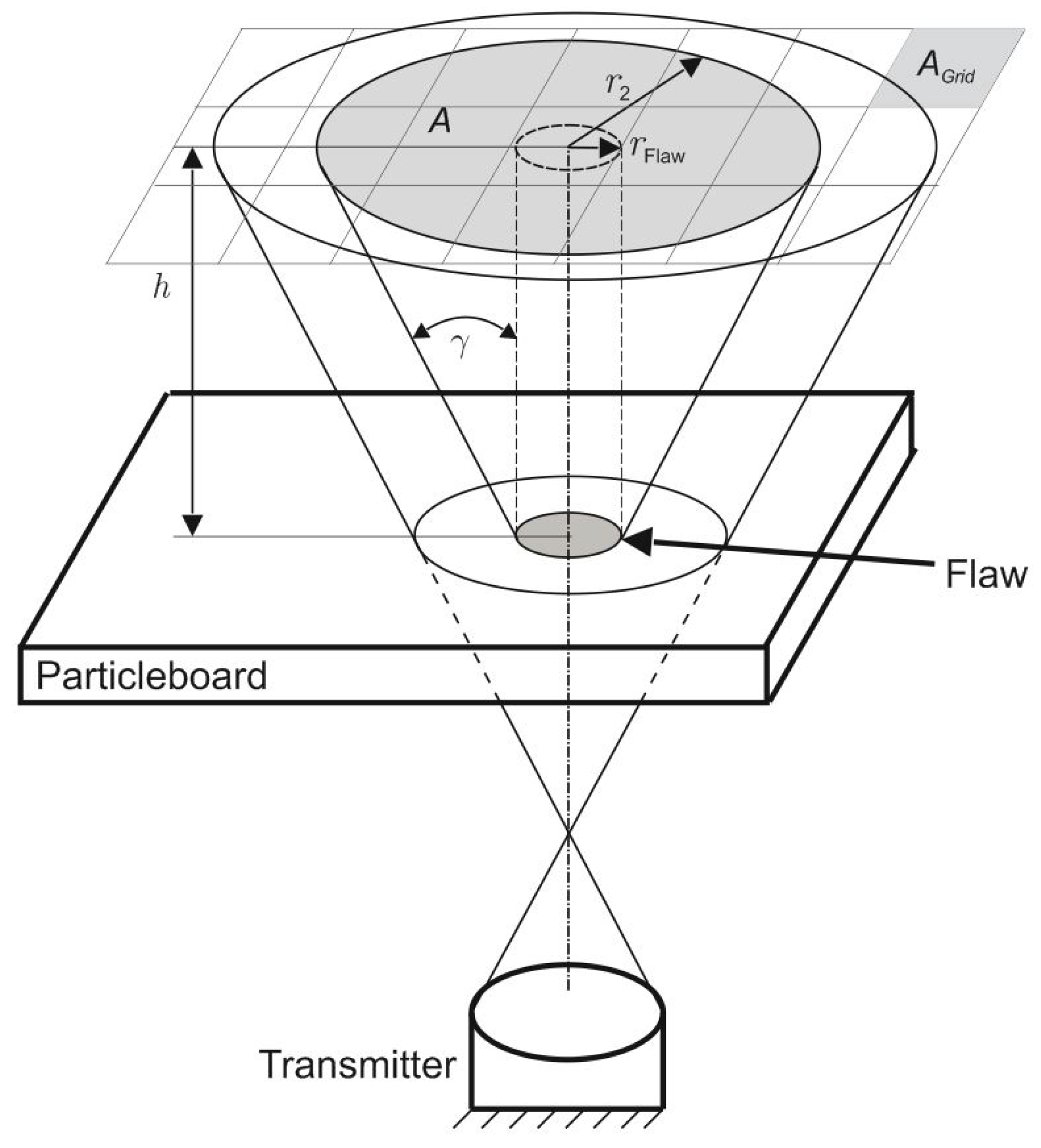
2.1. Experimental Setup

The test material was a commercially available wooden medium-density fiberboard (MDF) particleboard measuring hight = 800 mm, wide = 800 mm and thick = 20 mm. Pieces of paper were used as imitations of flaws, which is typically done for particleboards [17,22], instead of teflon tape, which is historically used for the inspection of CFRP or GFRP. These were circular with a diameter of 2, 4, 5, 10, and 20 mm (Figure 1). Paper was chosen because it is assumed to possess similar material properties to the wooden particleboard. When placing the pieces of paper on the particleboard, there is always a thin air film between the piece of paper and the particleboard. This air film serves as flaw imitation and causes a similar impedance change in the material properties as a real flaw in the wooden particleboard.

A standard Airmar pulse ultrasonic transducer was used as the transmitter. The used model AT50 has an operating frequency of approximately 50 kHz and an active diameter of approximately 45 mm. This transmitter was operated with 10 cycles of sinusoidal oscillations with an amplitude of 80 V at a repeating frequency of 1 Hz. The distance between the transmitter and the particleboard was 280 mm. The distance was therefore greater than the near field length (≈72 mm) of the transmitter in air at this frequency. The transmitter was fixed and did not move during the whole measurement. As a receiver, a Knowles microphone, SPU0410LR5H-QB, was used, which was selected as optimal for this experiment due to its very small construction and its recording frequency of up to 80 kHz. The wooden particleboard was also immovable. Air was used as a coupling medium between the transmitter and the particleboard and between the particleboard and the receiver. Accordingly, the microphone has to move for a C-scan. For this, it was attached to an XYZ traversing unit from RoboCylinder, which has a traverse path of x = 0–400 mm, y = 0–200 mm and z = 0–200 mm. The entire measuring setup was controlled by a standard computer. The XYZ traversing unit was connected via USB-connection to the PC and controlled via LabView program. The control of the transmitter and the signal recording of the microphone were carried out with an NI system. PXIe-1085 was used as chassis, and, for the communication between the NI system and the PC, the PXIe-8398 card was used. The PXIe-5171R card was used to record the measurement data with a maximum sampling frequency of 250 MHz on 8 channels. The frequency generator card PXIe-5423 was used to control the transmitter. To amplify the signal of the frequency generator, the power amplifier 1040L of the company E&I was used to generate the required 80 V amplitude. Various measuring grid point distances were investigated, but dx = dy was always used. Figure 2 depicts a schematic representation of the measurement setup, and Figure 3 depicts a representation of the experimental setup.

2.2. Mathematical Methods

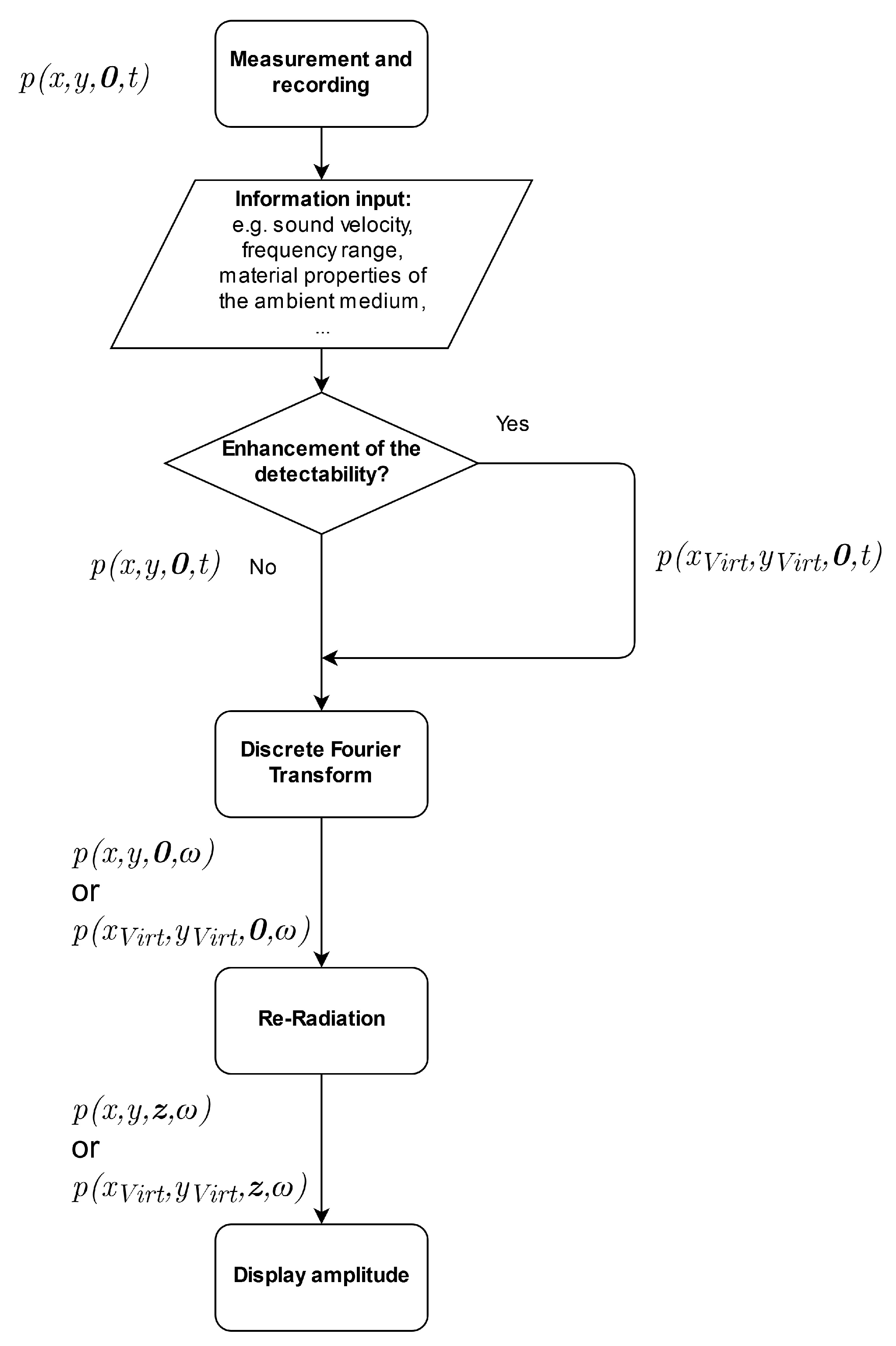
2.2.1. Re-Radiation

The re-radiation method is based on the Rayleigh–Sommerfeld diffraction integral. This is based on the wave equation:

$${▽}^{2}p-{\displaystyle \frac{1}{c^2}}{\displaystyle \frac{{\partial }^{2}p}{\partial t^2}}=0.$$

(1)

where p is the acoustic pressure, c the speed of sound, t the time, and ▽ is the nabla-operator. Sommerfeld has already shown [23] how the diffraction integral is obtained by applying Green’s theorem from the wave equation. This correlation from optics can also be applied to the acoustics of gaseous media and has already been used in in previous works [16,17,18,19,20,22], as well as in NDT, and is only briefly presented and explained here. The pressure value in the propagation plane (Figure 4) is the integral of the pressure value in the measuring plane multiplied by the derivative of the Green’s function. It can be understood as the sum of the respective parts of the measuring plane for the wave propagation to the propagation plane. The Rayleigh–Sommerfeld diffraction integral in the frequency domain in its unrestricted form is:

$$p(x,y,z,\omega )=2{\int }_{S}p(x^{\prime },y^{\prime },0,\omega ){\displaystyle \frac{\partial G}{\partial z}}\mathrm{d}{x}^{\prime }\mathrm{d}{y}^{\prime }.$$

(2)

It describes the integral of the acoustic pressure over an entire known area S multiplied by the derivative of the free space Green’s function. x, y, z are Cartesian coordinates. G is the free space Green’s function [23]:

$$G=-{\displaystyle \frac{{\mathrm{e}}^{(V\mathrm{i}k\sqrt{{(x-x^{\prime })}^2+{(y-y^{\prime })}^2+z^2})}}{4\pi \sqrt{{(x-x^{\prime })}^2+{(y-y^{\prime })}^2+z^2}}}=-{\displaystyle \frac{{\mathrm{e}}^{V\mathrm{i}kR}}{4\pi R}}.$$

(3)

In this equation, i is the complex unit, k is the wave number, and V is the propagation parameter and for the back propagation −1. R is the direct distance of one point in the known plane to one point in the propagation plane. The derivative of the free space Green’s function for the backward propagation is:

$${\displaystyle \frac{\partial G}{\partial z}}={\displaystyle \frac{z{\mathrm{e}}^{-\mathrm{i}kR}}{4\pi R^2}}\left({\displaystyle \frac{1}{R}}+\mathrm{i}k\right).$$

(4)

In order to solve the Rayleigh–Sommerfeld diffraction integral for practical applications, Delen [24] has suggested to performing the convolution in the wave number space because this is a very time efficient way to compute the integral numerically. Thus, the equation used here for the re-radiation method results in

$$p(x,y,z,\omega )\cong 2h^{2}p(x^{\prime },y^{\prime },0,\omega )\ast {\displaystyle \frac{z{\mathrm{e}}^{-\mathrm{i}kR}}{4\pi R^2}}\left({\displaystyle \frac{1}{R}}+\mathrm{i}k\right).$$

(5)

The asterisk is the convolution operator, and $h^2$ is the area around each point in the plane, as depicted in Figure 4.

Figure 5a depicts an airborne sound field that was calculated utilizing the re-radiation method. On the right side is the measuring plane, and the left side shows the surface of a particleboard that was excited with the transmitter; at the surface of the particleboard, there is a 20 mm flaw. The propagation plain is always the air layer directly above of the particleboard, like that shown in Figure 5b. All results of the re-radiation method are further depicted for a frequency range from 48 to 52 kHz.

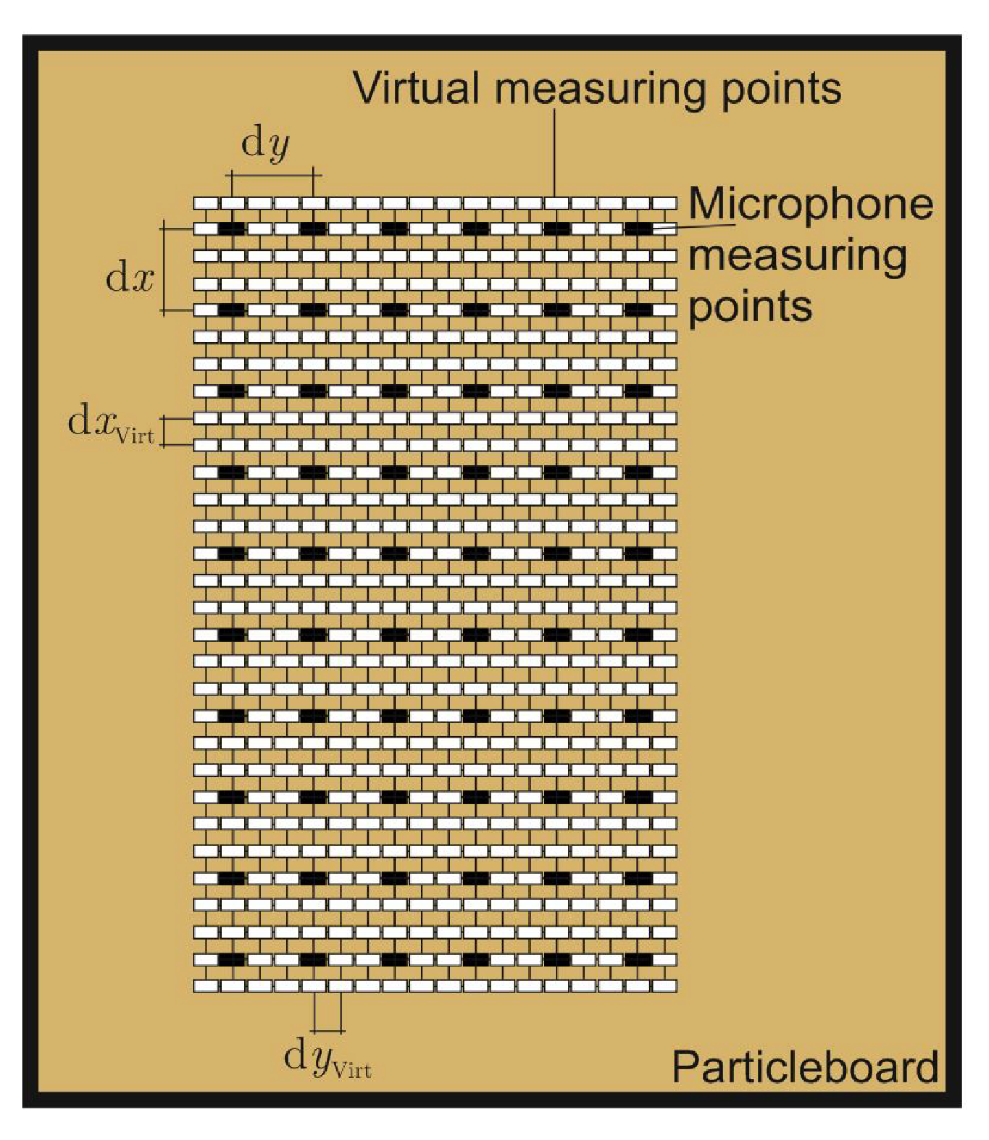
2.2.2. Virtual Refinement

The greatest potential for reducing the required measuring time is a reduction in the number of measuring grid points. We briefly explain what happens to the results of the C-scan by the re-radiation method when the measuring grid is coarsened. Figure 6 depicts the calculated surfaces of the particleboard, with and without different flaw sizes. The measuring grid point distance was always dx = dy = 2 mm, which is less than $\lambda /3$ ($\lambda \approx 6.8$ mm) for the C-scan. The circular shape of the main lobe of the transmitter is depicted as the red area in each diagram. The flaws were placed with its center at the position $x\approx 90$ mm and $y\approx 70$ mm. At a size of 4 mm, the flaws are visible and can be identified at the yellow, green, and blue area at the flaw position. An amplitude decrease caused by the larger flaws measuring 10 and 20 mm is depicted within the blue area. The flaw in the size of 2 mm cannot be recognized because it is smaller than the detectability limit, which means that the maximum detectability of flaws of the Rayleigh–Sommerfeld diffraction integral is in a size of $\lambda /2$ when $\lambda$ is the wavelength of the propagation medium [25,26]. Since the transmitter was operated with 50 kHz and the sound velocity of air is about 343 m/s, the wavelength is about 6.8 mm, and the 2 mm flaw is smaller than the maximum detectability.

With the measuring grid point distance of 2 mm, 10,201 measuring grid points had to be measured for such a large measuring window of 200 × 200 mm. Since each measurement needs 5 s, this is an enormous expenditure of time. Our proposed method to mitigate this large time expenditure is coarsening the measuring grid. Figure 7 depicts the results for no flaw and for the 20 mm flaw when the measuring grid get coarsened. Figure 7a,d are the “default” images. The top row is without a flaw, and below is with a 20 mm flaw. Figure 7b,e have a 10 mm measuring grid point distance, and Figure 7c,f a 14 mm grid point distance. The results in Figure 7b,e are influenced by much more noise. With some knowledge of the used transmitter, the circular form can be recognized.

The 20 mm flaw is identifiable. However, a red area at $y\approx 20$ mm can be seen due to a failure influenced back propagation due to less measuring grid points. The grid point distance is insufficient, and the images are not clear enough for a sufficient interpretation. When the measuring grid is coarsened down to the 14 mm grid, nothing can be detected. With this measuring grid point distance, only 196 measuring grid points need to be measured, reducing the experiment time by up to 98%.

The idea is to take these coarse grids and refine it in the measuring plane, as depicted in Figure 8. The black points refer to the measuring positions with the grid point distance of dx and dy. The white points are the virtual grid points; with them, the grid has the new virtual grid point distance of d$x_{Virt}$ and d$y_{Virt}$. The idea is to fill these virtual measuring grid points with transient interpolated data and then apply the re-radiation method. This is due to the flaws having different geometrical forms in reality and finding a uniform function which covers all imaginable forms is not target-oriented. Shown here are the different interpolation methods employed. The computation took place in MATLAB (MathWorks, Natick, MA, US) and the interpolation with the command interp3. In this work, the five interpolation methods (“linear”, “nearest”, “cubic”, “spline”, and “makima”) that this command already offers in MATLAB are used and compared.

Figure 9 (top row) depicts snapshots of the time data in the measuring plane. Figure 9a is the very time-consuming measurement with a measurement grid point distance of 2 mm without flaw. Figure 9b the measurement with a grid point distance of 14 mm. This measurement needs only a fraction of time as the one with the 2 mm grid point distance but with decreased detectability. The virtual measuring grid points are depicted in Figure 9c. Figure 9c is a refined image of Figure 9b using the interpolation method “nearest” to a 2 mm grid point distance. It can be seen that these are the same data, and the grid is refined by copying the data to the virtual measuring grid points. Figure 9 (bottom row) depicts the back propagated amplitude distribution on the top of the particleboard from the upper row data. Figure 9c is the “default” and Figure 9e with the coarse measuring grid point distance of 14 mm. Figure 9f is the result of the refined measuring grid of Figure 9c. The circular shape of the main lobe of the transmitter can be clearly identified.

Figure 10 shows a sequence of steps from the measurement of the pressure values to the final display of the pressure amplitude images. First, the measurement must be performed and the time data from each measurement point from the C-scan must be stored. This data can be stored as a 3D matrix, where two dimensions represent the space and one, the time. After that, various material constants must be specified for the procedure, such as the speed of sound of the air, which can be calculated according to Cramer [27] after measuring humidity, air pressure, and temperature. In the experiments we carried out, the speed of sound of the air was 343 m/s. After entering the important parameters, the decision follows whether the detectability should be increased or not. If the detectability is to be increased, because a rough measuring grid was used, the existing 3D matrix must be enlarged in the two dimensions representing the space and filled with the interpolation results. This is followed by a discrete Fourier transformation and the application of re-radiation method. As a result, the pressure amplitudes at the previously defined distance to the measuring plane are displayed. The aforementioned method is used in the following section for the identification of flaws.

3. Results

In the first subsection, the results of our refinement method are presented using the example of the 20 mm flaw. The four interpolation methods are compared with each other and with the reference. It is investigated in this study how large the error of the reconstruction is and how much time can be saved. In the second subsection, the sensitivity of the measurement grid point distance in respect to the identification of the flaw size with a refined grid is investigated.

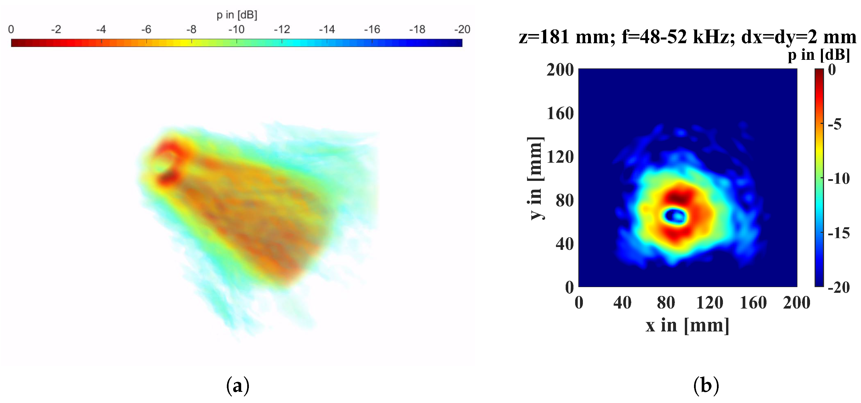
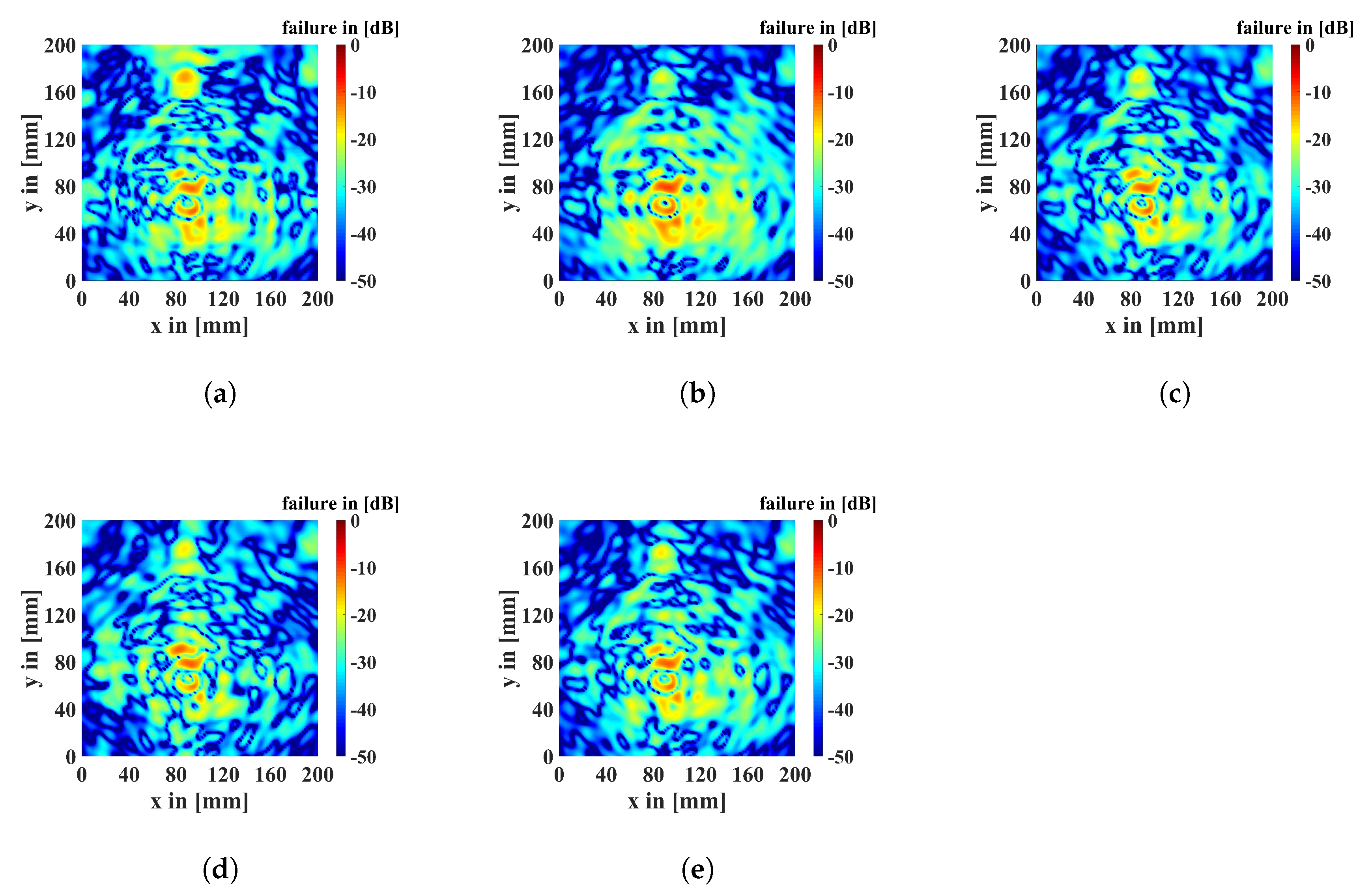
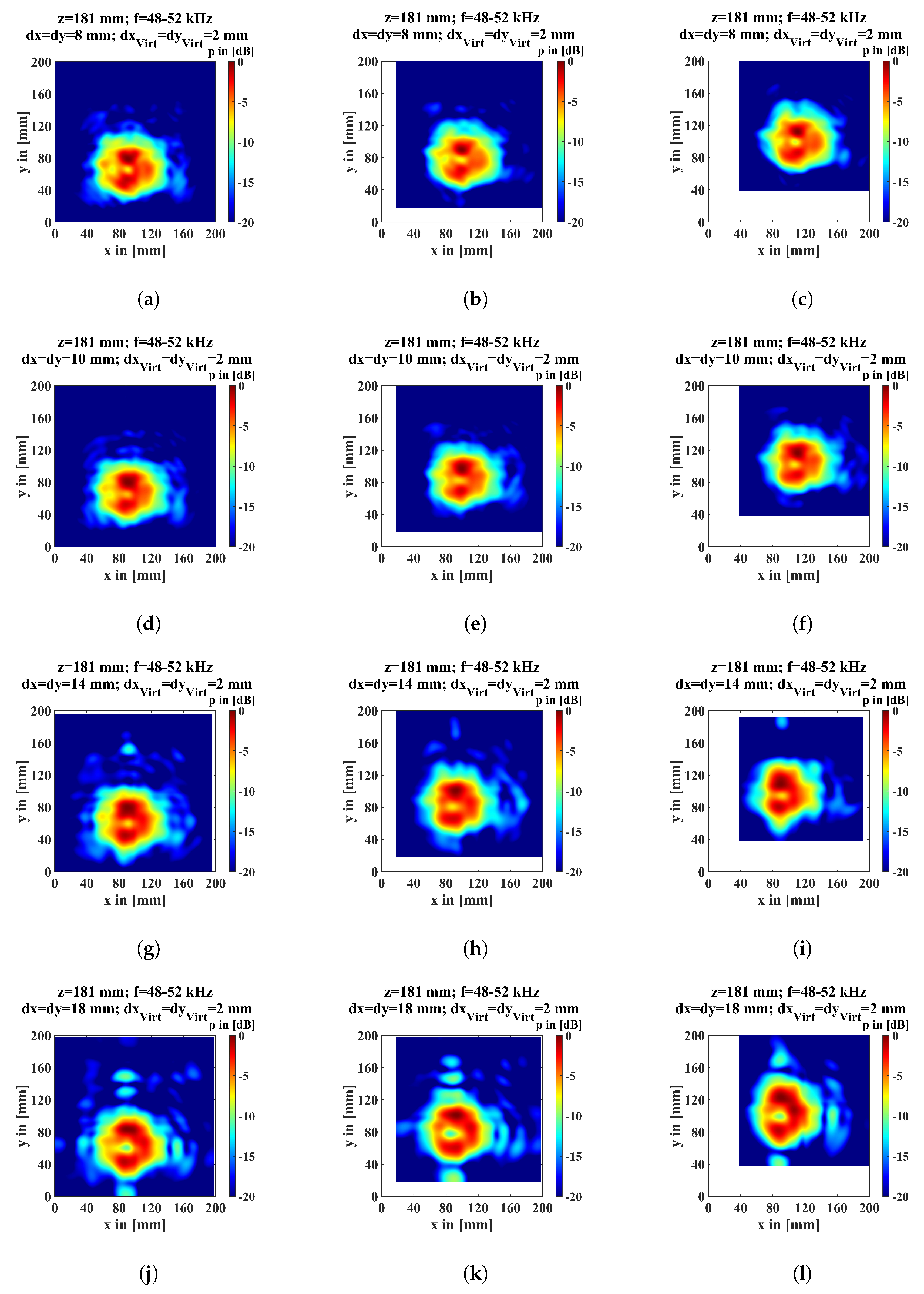
3.1. Detectability Enhancement with Coarse Measurement Grid

Without refining the coarse measuring grid point distance of 14 mm, the time data, a section of which is shown in Figure 9b, becomes a non-interpretable image (see Figure 7). However, to save time during the experiment, we take this data and interpolate it to a finer grid. For this, we use different interpolation methods. In order to enable an optical direct comparison of the individual methods with a result that is not refined but finely measured, Figure 11 shows the 6 images of the back propagated sound fields on the surface of the particleboard. Figure 11a shows the result if the measuring grid point distance is 2 mm. For Figure 11b–f, a measuring grid point distance of 14 mm was measured and the time data interpolated to a gird point distance of 2 mm. The round shape of the transmitter can be seen in every image. The 20 mm flaw can also be clearly identified in each image. Figure 11c, interpolated linearly, shows the lowest visible noise. In contrast, Figure 11b shows the highest noise when interpolated with the “nearest” method. Compared to other interpolation methods, the amplitude drop in Figure 11c is not as stark. This is shown through the colored areas of yellow through green in the area of the flaw. Moreover, a dark blue color is not present as compared to the other images. Figure 11 clearly shows that this procedure is promising.

Since the visual differences are difficult to compare directly, the following error image is calculated in each case:

$$ErrorImage=20{\log }_{10}\left({\displaystyle \frac{\left|InterpolatedImage-DefaultImage\right|}{DefaultImage}}\right).$$

(6)

These images are depicted in Figure 12. The difference is so small that it is not recognizable on the −20 dB scale (that was used in all other figures) a −50 dB scale was used instead.

These images depict that there are significant differences. With the interpolation method “nearest” a large error at around y = 170, x = 90. Using the interpolation method “linear”, the largest error is seen in the area of the 20 mm flaw. Figure 12c–e depict similarity in errors. All images present a large part of their errors in the area of the flaw, but previous images (see Figure 11) show that these are not decisive in the flaw identification.

To decide which of the images in Figure 11 are the best reproduction of the “default” image, the sum of all pixel values in Figure 12 are calculated, and the largest absolute value is determined to be the best reproduction. In this case, the “spline” interpolation is the best reproduction (see Figure 11e and Figure 12d). In Figure 13, these values depicted are related to the best reproduction. It can be seen that all methods have similar accuracy values. It is shown that the interpolation method “linear” is the worst reproduction.

Since time efficiency is a main objective, the computation time for the interpolation is given in Figure 14. Figure 14 depicts the needed time for the evaluation of the measurement results related to the “default” time. It can be seen in Figure 14 that each interpolation method needs approximately 500% evaluation time related to the “default” time. Only the “makima” interpolation method needs 1200% extra time for the evaluation; in comparison to Figure 13, this is not the best reproduction. The presented example has a measurement time reduction of 98%, equivalent to up to 10 hours of time saved. An extra evaluation time of 1200% is approximately 1 min.

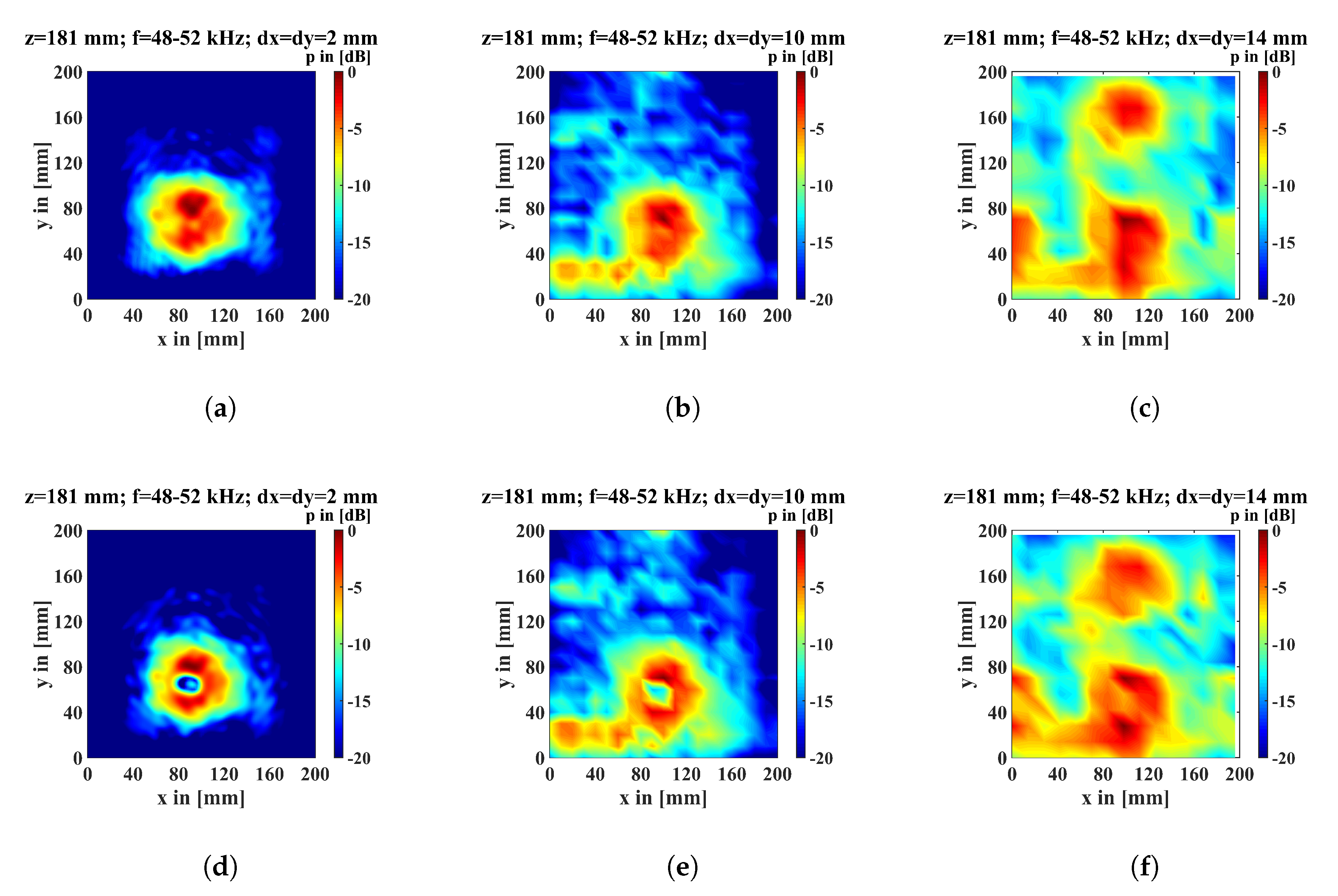
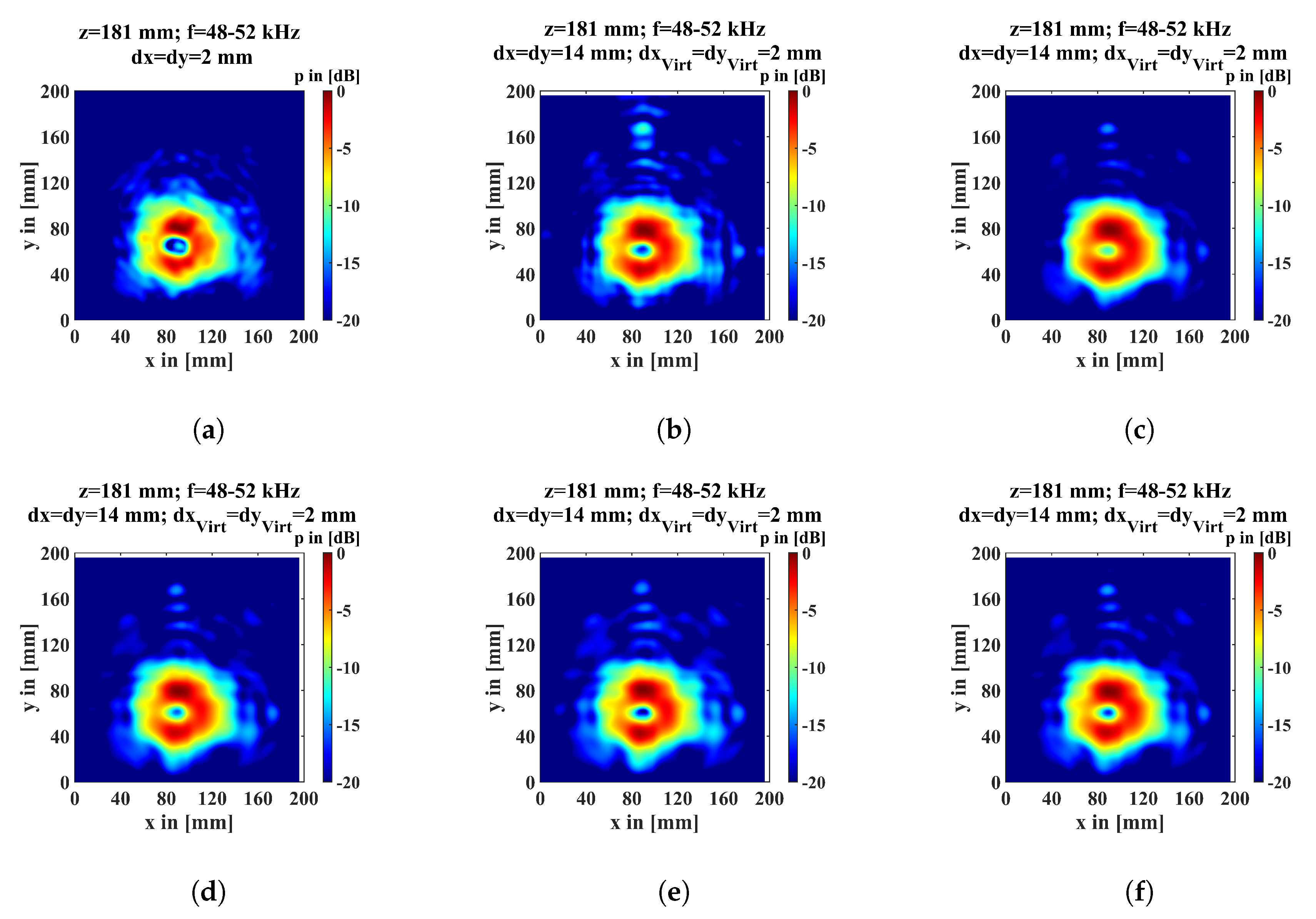
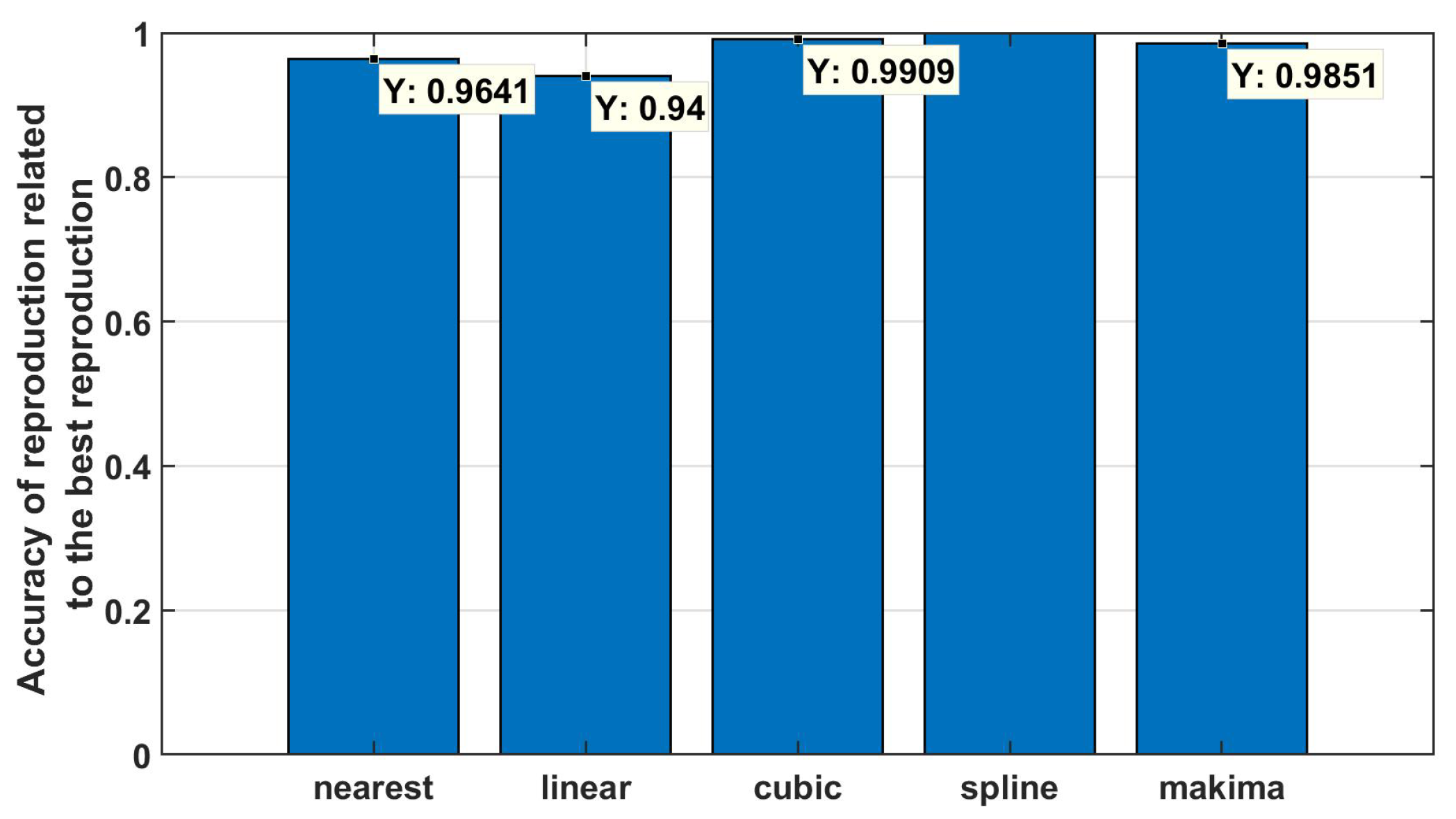
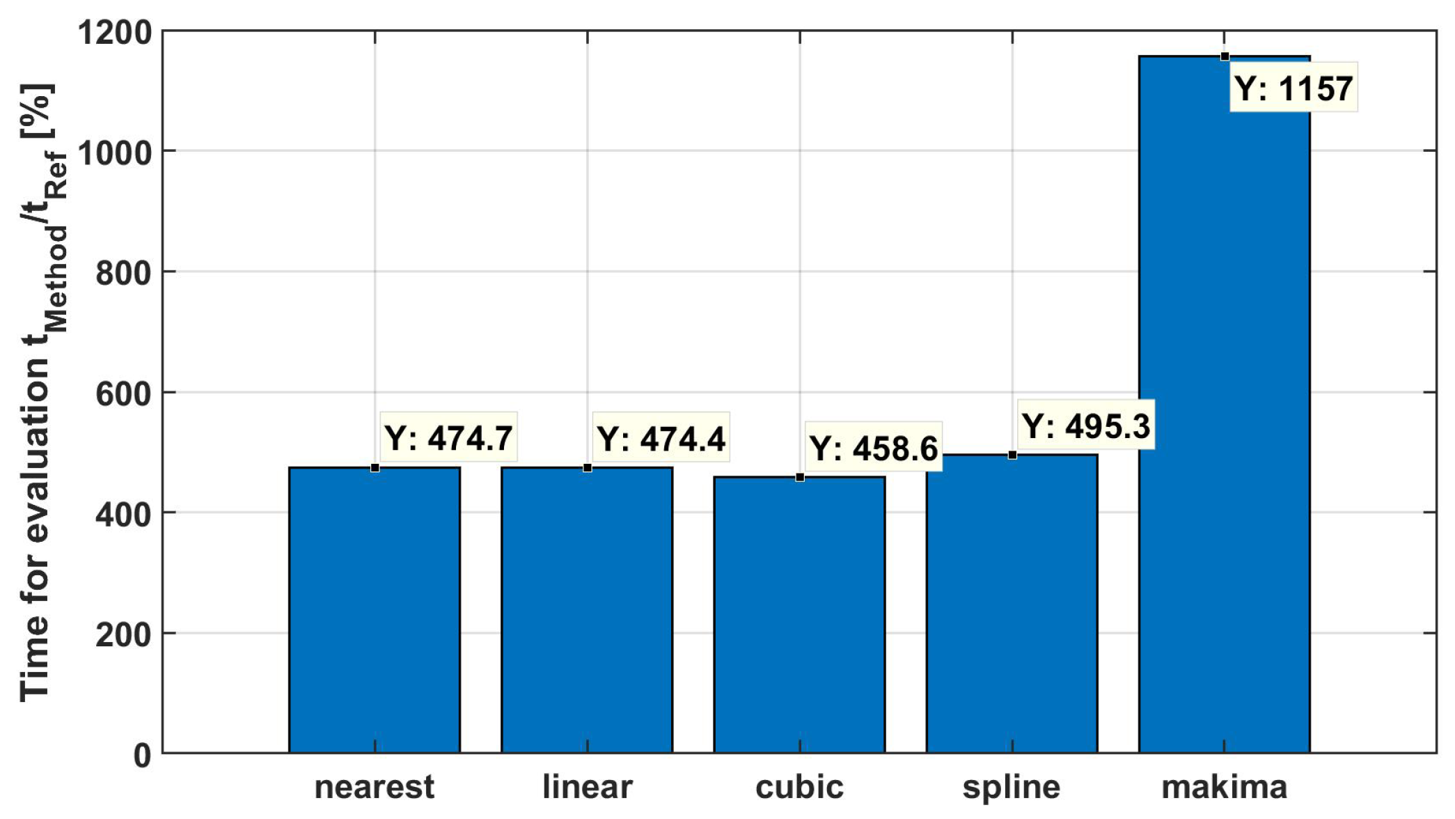
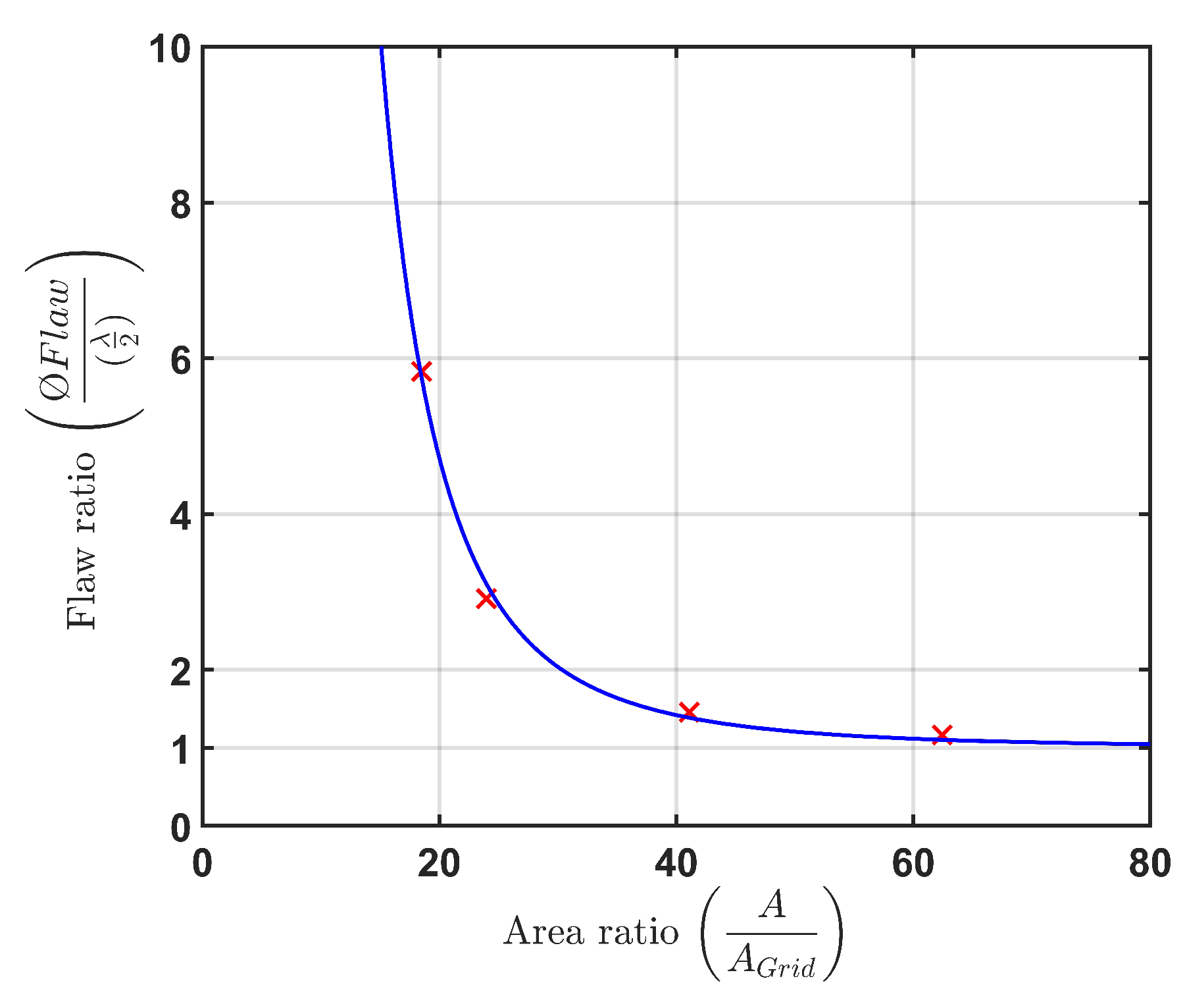
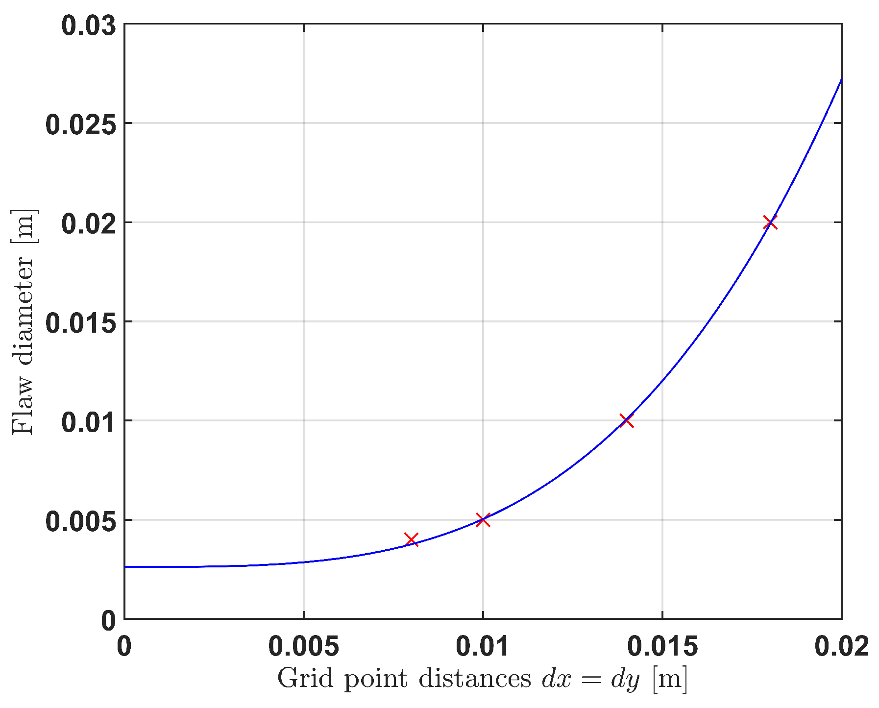
3.2. Sensitivity of the Measurement Grid Point Distance in Respect to the Identification of the Flaw with a Refined Grid

Starting from the previously determined interpolation method “spline” for the best reproduction, we will now examine how coarse the measuring grid may be in order to obtain a well-interpretable detectability. It is assumed here that a certain number of real measured points must be present in the measuring surface which are in the sound field within the sphere of influence of the flaw. Therefore, it is indispensable to know the influence area of the flaw in the measured plane. To determine it, the following points are assumed:

• The opening angle of the sound field of the main lobe does not change.
• The flaw located behind the sound field shows its influence only in the sound field considering the opening angle of the main lobe.

The area of the sound field within the area of influence of the flaw is given in Figure 15. The area of the used circular flaws can be calculated from the truncated cone using the assumptions made. For this purpose, the opening angle of the transmitter is determined according to Krautkrämer [28], and the area is calculated:

$$A=\pi r_2^2=\pi {(\tan (\gamma )h+r_{\mathrm{Flaw}})}^2=\pi {(\tan (\arcsin (1.22{\displaystyle \frac{\lambda }{D_{\mathrm{Trans}}}}))h+r_{\mathrm{Flaw}})}^2,$$

(7)

where $\gamma$ is the opening angle, $r_2$ is the radius of the flaw influenced sound area in the measuring plane, h the distance between the particleboard and the measuring plane, $r_{\mathrm{Flaw}}$ the radius of the circular flaw, and $D_{\mathrm{Trans}}$ the diameter of the transmitter.

With knowledge of the area of influence of the flaw, it is now possible to check how coarse the measuring grid can be in order to identify a corresponding flaw. It is clear that, above a certain size, not only does the grid point distance of the measuring grid play a role, but also the position of the measuring grid points in relation to the position of the flaw. With this method, we ensure that the desired flaw size can also be identified with the desired coarse measuring grid. Therefore, we have shifted the measuring grid in relation to the position of the flaw in 2 mm steps by up to 40 mm in x- and y-direction. In the process, we have continuously coarsened the measuring grid and checked at which measurement grid point distance the flaw can still be identified at each position of the measuring grid. Due to the coarsened grid and the interpolation, the position of the flaw in the result image can lightly shift. Shown in Figure 16 are the results of the coarsest identified measuring grid of the different flaws with different measuring grid positions. Each line shows that the flaw can be roughly identified. At one grid position better than at another, it is always possible to identify the flaw. It has been shown that, for the 4 mm flaw (Figure 16, first row), an 8 mm grid is sufficient to identify it; for the 5 mm flaw (Figure 16, second row), a 10 mm grid is sufficient; for the 10 mm flaw (Figure 16, third row), a 14 mm grid; and for the 20 mm flaw (Figure 16, fourth row), an 18 mm grid is sufficient. As expected, there is increased noise with a coarser grid because, if there is only one measuring point which is strongly afflicted with noise, this affects the results more and more the less real measuring points are present for the interpolation.

On the basis of this data, we determined a function that represents the limit of the detectable flaw size relative to the detectability limit with the flaw influenced area in the measuring plane relative to the measuring grid point distance. This is shown in Figure 17. The function is the following equation:

$$Fla{w}_{ratio}\left({\displaystyle \frac{A}{A_{Grid}}}\right)=45390{\left({\displaystyle \frac{A}{A_{Grid}}}\right)}^{-\pi }+1.$$

(8)

It was created as an interpolation function of the specific maximum detectability. This is depicted in Figure 17 as the blue curve. The red crosses are the maximum measuring grid point distance associated with the flaw sizes. The maximum detectability with the re-radiation method of $\frac{\lambda }{2}$ is there at 1. This function asymptotically drops to the detectability limit but never reaches it. The values above the curve can thus be used for good identification of flaws with this method. To know if the desired measuring grid is sufficient to determine flaws up to a certain diameter, one could calculate the range of influence of the smallest expected flaw size with Equation (7) and divide it by the area of one square of the measuring grid. For values/data points above the blue line in Figure 17, this method is able to reliably identify flaws, regardless of the position of the measuring grid relative to the flaw.

For the special case presented here, Figure 18 depicts the flaw size with the measuring grid size. The whole area above the blue curve can be easily evaluated with this method. The red crosses are the measurement data used for this purpose. It can be clearly recognized that, for flaws that are $<\lambda$, measuring grid point distances of $>\frac{\lambda }{3}$ can be used.

4. Discussion

We have shown that, even with a very coarse measuring grid, it is possible to detect flaws. By using the interpolation on the 3D data set of the C-scan, it is possible to refine a coarse measuring grid to a fine measuring grid. Thus, more terms can be considered in the numerical evaluation of the Rayleigh–Sommerfeld diffraction integral. Because the local affiliation of the terms remains considered by the derivation of the Green’s function, a result image is generated which has a higher detectability of flaws than if the same measurement window would work without interpolated measurement points. We have shown that up to 98% of the experiment time can be saved in this way. With the different interpolation methods, it has been shown that, in the example presented here, the “spline” method can be used for the lowest error in the reproduction. The “nearest” interpolation method with its reproduction of the image is only about 4% worse than the “spline” method and takes less time to evaluate. If you think of the arithmetic operations behind it, we suggest the interpolation method “nearest”. This method only describes the copying of the data to surrounding points. If one wanted to automate these methods, then “nearest” is certainly the most favorable method. In relation to “spline” interpolation, we have shown the dependence of the measuring grid position on the position of the flaw, thereby determining the coarsest measuring grids for which a clear identification of the flaws is still possible. We have shown that, for flaws with sub wavelength sizes, a measuring grid point distance of $>\frac{\lambda }{3}$ can be used. On the basis of this, Equations (7) and (8) and Figure 17 give the possibility of adjusting the measuring grid to the desired flaw size prior to the actual measurement. We are convinced that, on further developments of the proposed method in future investigations, it will be possible for residual stresses/locational effects of the identified flaw areas to be quantified into strength, lifetime predictions. The proposed method is not only time efficient but reduces resources and energy expenditure, as well.

References

1. Sokolov, S.Y. On the problem of the propagation of ultrasonic oscillations in various bodies. Elek. Nachr. Tech. 1929, 6, 454–460. [Google Scholar]
2. Fleming, M.R.; Bhardwaj, M.C.; Janowiak, J.J.; Shield, E.J.; Roy, R.; Agrawal, D.K.; Bauer, L.S.; Miller, D.L.; Hoover, K. Noncontact ultrasound detection of exotic insects in wood packing materials. For. Prod. J. 2005, 55, 33–37. [Google Scholar]
3. Chimenti, D.E. Review of air-coupled ultrasonic materials characterization. Ultrasonics 2014, 54, 1804–1816. [Google Scholar] [CrossRef] [PubMed]
4. Hillger, W.; Bühling, L.; Ilse, D. Review 0f 30 years ultrasonic systems and developments for the future. In Proceedings of the 11th European Conference on Non-Destructive Testing (ECNDT 2014), Prague, Czech Republic, 6–10 October 2014. [Google Scholar]
5. Dunky, D.; Niemz, P. Theorie und Grundlagen der Verleimung und der Prüfung von Holzwerkstoffen. In Holzwerkstoffe und Leime; Springer: Berlin/Heidelberg, Germany, 2002; pp. 615–644. ISBN 978-3-642-62754-5. [Google Scholar]
6. Schiebold, K. Zerstörungsfreie Werkstoffprüfung—Ultraschallprüfung; Springer: Berlin/Heidelberg, Germany, 2015; ISBN 978-3-662-44699-7. [Google Scholar]
7. Stößel, R. Air-Coupled Ultrasound Inspection as a New Non-Destructive Testing Tool for Quality Assurance. Ph.D. Thesis, Universität Stuttgart, Stuttgart, Germany, 2003. [Google Scholar]
8. Dahmen, S.; Ketata, H.; Ghozlen, M.H.B.; Hosten, B. Elastic constants measurement of anisotropic Olivier wood plates using air-coupled transducers generated Lamb wave and ultrasonic bulk waves. Ultrasonics 2010, 50, 502–507. [Google Scholar] [CrossRef] [PubMed]
9. Fang, Y.; Lin, L.; Feng, H.; Lu, Z.; Emms, G.W. Review of the use of air-coupled ultrasonic technologies for nondestructive testing of wood and wood products. Comput. Electron. Agric. 2017, 137, 79–87. [Google Scholar] [CrossRef]
10. Bucur, V. Delamination detection in wood—Based composites, a methodological review. In Proceedings of the 20th International Congress on Acoustics (ICA 2010), Cape Town, South Africa, 7–12 March 2010; pp. 835–843, ISBN 978-1-61782-745-7. [Google Scholar]
11. Döring, D. Luftgekoppelter Ultraschall und Geführte Wellen für die Anwendung in der Zerstörungsfreien Werkstoffprüfung. Ph.D. Thesis, Universität Stuttgart, Stuttgart, Germany, 2011. [Google Scholar]
12. Matthies, K.; Gohlke, D. Der Ultraschall-Volumenscan als Werkzeug zur Prüfung komplizierter Geometrien und komplexer Gefüge. In Proceedings of the DGZfP—Jahrestagung, Fürth, Germany, 14–16 May 2007; Volume 57, ISBN 978-3-931381-98-1. [Google Scholar]
13. Krautkrämer, J.; Krautkrämer, H. Bild und rekonstruktionsverfahren. In Werkstoffprüfungen mit ultraschall; Springer: Berlin/Heidelberg, Germany, 1986; Volume 5, pp. 262–288. [Google Scholar]
14. Hoffmann, M.; Unger, A.; Ho, M.-C.; Park, K.K.; Khuri-Yakub, B.T.; Kupnik, M. Volumetric characterization of ultrasonic transducers for gas flow metering. In Proceedings of the 2013 IEEE International Ultrasonics Symposium (IUS), Prague, Czech Republic, 21–25 July 2013; pp. 1315–1318. [Google Scholar] [CrossRef]
15. Neild, A.; Hutchins, D.A.; Robertson, T.J.; Davis, L.A.J.; Billson, D.R. The radiated fields of focussing air-coupled ultrasonic phased arrays. Ultrasonics 2005, 43, 183–195. [Google Scholar] [CrossRef] [PubMed]
16. Marhenke, T.; Sanabria, S.J.; Chintada, B.R.; Furrer, R.; Neuenschwander, J.; Goksel, O. Acoustic field characterization of medical array transducers based on unfocused transmits and single-plane hydrophone measurements. Sensors 2019, 19, 863. [Google Scholar] [CrossRef] [PubMed] [Green Version]
17. Marhenke, T.; Sanabria, S.J.; Twiefel, J.; Furrer, R.; Neuenschwander, J.; Wallaschek, J. Three dimensional sound field computation and optimization of the delamination detection based on the re-radiation. In Proceedings of the 12th European Conference on Non-destructive Testing (12th ECNDT), Gothenburg, Sweden, 11–15 June 2018; ISBN 978-91-639-6217-2. [Google Scholar]
18. Sanabria, S.J.; Marhenke, T.; Furrer, R.; Neuenschwander, J. Calculation of volumetric sound field of pulsed air-coupled ultrasound transducers based on single-plane measurements. IEEE Trans. Ultrason. Ferroelectr. Freq. Control. 2018, 65, 72–84. [Google Scholar] [CrossRef] [PubMed]
19. Schmelt, A.S.; Marhenke, T.; Twiefel, J. Identifying objects in a 2D-space utilizing a novel combination of a re-radiation based method and of a difference-image-method. In Proceedings of the 23rd International Congress on Acoustics (ICA 2019), Aachen, Germany, 9–13 September 2019; ISBN 978-3-939296-15-7. [Google Scholar]
20. Tsysar, S.A.; Sapozhnikov, O.A. Ultrasonic holography of 3D objects. In Proceedings of the IEEE International Ultrasonics Symposium (2009 IEEE IUS), Roma, Italy, 20–23 September 2009; pp. 737–740. [Google Scholar]
21. Schmerr, L.W.; Song, S.-J. A Rayleigh–Sommerfeld Integral Transducer Model. In Ultrasonic Nondestructive Evaluation Systems—Models and Measurements; Springer: New York, NY, USA, 2007; pp. 134–137. [Google Scholar]
22. Marhenke, T.; Neuenschwander, J.; Furrer, R.; Zolliker, P.; Twiefel, J.; Hasener, J.; Wallaschek, J.; Sanabria, S. Air-coupled ultrasound time reversal (ACU-TR) for subwavelength non-destructive imaging. IEEE Trans. Ultrason. Ferroelectr. Freq. Contr. 2019. [Google Scholar] [CrossRef] [PubMed]
23. Sommerfeld, A. Optics: Lectures on Theoretical Physics. In Optics: Lectures on Theoretical Physics; Academic: New York, NY, USA, 1964; p. 197. [Google Scholar]
24. Delen, N.; Hooker, B. Free-space beam propagation between arbitrarily oriented planes based on full diffraction theory: A fast Fourier transform approach. J. Opt. Soc. Am. A 1998, 15, 857–867. [Google Scholar] [CrossRef]
25. Simonetti, F. Multiple scattering: The key to unravel the subwavelength world from the far-field pattern of a scattered wave. Phys. Rev. 2006, 73, 036619-1–036619-13. [Google Scholar] [CrossRef] [PubMed]
26. Wolf, E. Three-dimensional structure determination of semi-transparent objects from holographic data. Opt. Commun. 1969, 1, 153–156. [Google Scholar] [CrossRef]
27. Cramer, O. The variation of the specific heat ratio and the speed of sound in air with temperature, pressure, humidity, and CO2 concentration. J. Acoust. Soc. Am. 1993, 93, 2510–2516. [Google Scholar] [CrossRef]
28. Krautkrämer, J.; Krautkrämer, H. Schallfeld des ebenen, kreisförmigen Kolbenschwingers. In Werkstoffprüfungen mit ultraschall; Springer: Berlin/Heidelberg, Germany, 1986; Volume 5, pp. 73–80. [Google Scholar]
Figure 1. Flaw imitations with a diameter of 20, 10, 5, 4, and 2 mm, from left to right, with a thickness of 0.6 mm.
Applsci 10 01155 g001
Figure 2. Schematic experimental setup with a flaw imitation at the top of the wooden particleboard.
Applsci 10 01155 g002
Figure 3. Experimental setup with a flaw imitation at the top of the wooden particleboard. NI = National Instruments.
Applsci 10 01155 g003
Figure 4. Schematic representation of the re-radiation method.
Applsci 10 01155 g004
Figure 5. (a) Back propagated amplitude pressure field of several planes in a distance of 1 mm. At the rigth side is the measuring plane, and depicted at the left side is the air layer directly above the top surface of the particleboard with a 20 mm flaw. (b) Back propagated amplitude pressure field at the top of the particleboard with a 20 mm flaw.
Applsci 10 01155 g005
Figure 6. Back propagated amplitudes at the top of the particleboard. (a) Without a flaw, (b) with a 2 mm flaw, (c) with a 4 mm flaw, (d) with a 5 mm flaw, (e) with a 10 mm flaw, and (f) with a 20 mm flaw.
Applsci 10 01155 g006
Figure 7. Back propagated amplitude with different measuring grid point distances. (Top row) With no flaw on the particleboard; (lower row) with a 20 mm flaw. (a,d) with a 2 mm measuring grid, (b,e) with a 10 mm measuring grid, and (c,f) with a 14 mm measuring grid.
Applsci 10 01155 g007
Figure 8. The idea of virtual measuring grid points.
Applsci 10 01155 g008
Figure 9. The upper row depicts snapshots of the time data in the measuring plane with different measuring grid point distances. (a) “Default” measuring grid with dx = dy = 2 mm. (b) The coarse measuring grid with a grid point distance of dx = dy = 14 mm; (c) the data from (b) refined with the interpolation method “nearest” to a measuring grid d x V i r t = d y V i r t = 2 mm. The lower row depicts the back propagated amplitude distribution at the top of the particleboard. (d) “default” measuring grid with dx = dy = 2 mm. (e) The coarse measuring grid with a grid point distance of dx = dy = 14 mm and (f) refined with the interpolation method “nearest” to a measuring grid d x V i r t = d y V i r t = 2 mm.
Applsci 10 01155 g009
Figure 10. Practical realization and implementation of the re-radiation method with the increase of the detectability.
Applsci 10 01155 g010
Figure 11. Back propagated amplitude at the top of the particleboard. (a) The “default” image measured with a 2 mm grid; the rest were measured with a 14 mm grid and refined to a 2 mm grid. (b) Interpolation method “nearest”. (c) Interpolation method “linear”. (d) Interpolation method “cubic”. (e) Interpolation method “spline”. (f) Interpolation method “makima”.
Applsci 10 01155 g011
Figure 12. Error images of the different interpolation methods for the refining of the measurement values related to the “default” image. Interpolation method (a) “nearest”; (b) “linear”; (c) “cubic”; (d) “spline” and (e) “makima”.
Applsci 10 01155 g012
Figure 13. Accuracy of the reproduction related to the best reproduction of the individual interpolation methods.
Applsci 10 01155 g013
Figure 14. Time for the evaluation of the different refinement methods related to the “default” evaluation time.
Applsci 10 01155 g014
Figure 15. Schematic representation of the sound fields and the measuring grid.
Applsci 10 01155 g015
Figure 16. Results of the coarsest identified measuring grid of the different flaws with different measuring grid position. (ac) The 4 mm flaw with 8 mm grid point distance, (df) the 5 mm flaw with 10 mm grid point distance, (gi) the 10 mm flaw with 14 mm grid point distance, and (jl) the 20 mm flaw with 18 mm grid point distance. In the first column, with the default measuring grid position. In the second column, with a 20 mm shifted measuring grid and in the third column with a 40 mm shifted measuring grid.
Applsci 10 01155 g016
Figure 17. Determinable flaw ratio in relation to the area ratio.
Applsci 10 01155 g017
Figure 18. Determinable flaw size in relation to the grid point distance.
Applsci 10 01155 g018