Influence of Vertical Fastener Stiffness on Rail Sound Power Characteristics: Numerical Study and Field Measurement

Abstract

The aim of this paper is to investigate the influence of vertical fastener stiffness on the sound power characteristics of rail rolling noise. The rail mobility is obtained by using the Timoshenko-beam track model and the spectral element method. The decay rate is obtained by using the periodic track model and the spectral transfer matrix method. Then, the simulation results of the rail mobility and the decay rate are used to calculate the sound power level of the rail subjected to a harmonic point excitation. Furthermore, the influence of vertical fastener stiffness on the rail sound power level is investigated. Finally, field measurements of the rail accelerance and the decay rate are performed to verify the accuracy of models and calculation methods. The results show that the sound power level of the rail subjected to a harmonic point excitation increases with the increase of the frequency and peaks at the center frequency of 800 Hz. When the vertical fastener stiffness decreases from 50 kN/mm, the rail sound power level below the center frequency of 200 Hz gets increased. The increase of the sound power level is most significant at the center frequency which is close to the decreased vertical rail resonance frequency, because in the corresponding one-third octave band the rail mobility amplitude increases significantly while the decay rate decreases considerably. The simulations of the rail accelerance and the decay rate both coincide well with the measurements.

1. Introduction

Ground-borne vibrations induced by subway trains can have terrible effects on buildings, residents and instruments [1]. As comfortable urban living environments have become great concerns, track vibration–mitigation techniques attract a lot of attention. In order to mitigate ground-borne vibrations, fasteners of low vertical stiffness have been used to weaken the coupling between the rail and the sleeper, which can prevent vibrations transmitted from the rail to the infrastructure. Nevertheless, low stiffness reduces the decay of vibration with distance along the rail and leads to an increase of rolling noise radiated by the rail, causing severe noise problems. Rail sound power reflects total sound energy radiated by the rail per unit time, which does not depend on a receiver location. Therefore, investigating the influence of vertical fastener stiffness on the sound power characteristics of rail rolling noise is of great help to solve the problems of subway vibrations and noises.

The rail sound power is determined by the vibration velocity amplitude, the decay rate (DR) and other factors [2]. There have been many studies on the rail vibration characteristics which are essential to the insight into the rail sound power. Knothe and Wu [3] utilized a frequency-domain analysis to explain the receptance behaviors of a railway track. Kaewunruen and Remennikov [4] used the impact excitation technique to carry out the field investigations for the dynamic properties of the railway track. Oregui et al. [5] built whole- and half-track finite element models to investigate the vertical dynamic behaviors of railway tracks with monoblock sleepers. Arlaud et al. [6] used a new frequency-domain numerical method to study the frequency response of a railway ballast track and performed low-frequency receptance measurements.

The DR reflects the attenuation characteristics of rail vibrations in the longitudinal direction and controls the effective radiating length of the rail. Jones et al. [7] used simulations and measurements of frequency response functions to investigate DRs of different track structures. Squicciarini et al. [8] built a Timoshenko beam model to obtain the DR of an infinite beam on the continuous two-layer foundation. Betgen et al. [9] established a finite element model of the ballast track to consider the influences of section deformation and discrete supports on the DR. Li et al. [10] used the semi-analytical finite element method to obtain the DRs of a continuously supported rail.

The rail sound power has also been investigated by the previous works. Vincent et al. [11] used TWINS (Track-Wheel Interaction Noise Software) to calculate the total A-weighted sound power level of rail rolling noise in different calculation cases, and analyzed the influence of vertical fastener stiffness on the total A-weighted sound power level. However, the influence of vertical fastener stiffness on the rail sound power level at different frequencies is not investigated in that literature. Zhang et al. [12] predicted the sound radiation of a railway rail in close proximity to a ground by the boundary element method in two dimensions, paying no attention to the influence of vertical fastener stiffness. Thus, the influence of vertical fastener stiffness on the frequency-domain characteristics of rail sound power requires further studies.

The spectral element method (SEM) is a wave-based frequency-domain analysis method with high precision. The procedures of the SEM and the conventional finite element method (FEM) are similar. The SEM firstly divides a whole structure into a series of spectral elements and then assembles the spectral stiffness matrix of the whole structure with the spectral element stiffness matrixes [13]. It is noteworthy that the spectral element stiffness matrix is determined by substituting the exact wave solution into the governing differential equations. Both the element stiffness matrix and shape functions in the SEM are frequency-dependent while those in the FEM are only functions of the coordinates. In addition, the size of the spectral element has no influence on the calculation precision. A long and uniform member can be modeled with only one spectral element [14]. Therefore, the computation time and the number of degrees of freedom are both reduced.

The spectral transfer matrix method (STMM) [15] is the combination of the SEM and the transfer matrix method. The advantages of two methods can bring the superiority to the STMM in solving the vibration problems for a one-dimensional periodic structure. However, not all the nodes of a complicated periodic structure are located at two sides of the model, i.e., some nodes may be in the middle of the model. To build the transfer relation between two ends, the STMM should be improved by removing unnecessary degrees of freedom in the middle of the model. Recently, the SEM and the STMM have been adopted to study the transmission characteristics of vertical rail vibrations in the ballast track [16].

In this paper, the SEM and the STMM are adopted to investigate the rail sound power characteristics. The rail mobility is obtained by using the Timoshenko-beam track model and the SEM. The decay rate is obtained by using the periodic track model and the STMM. Then, the simulation results of the rail mobility and the decay rate are used to calculate the sound power level of the rail subjected to a harmonic point excitation. Furthermore, the influence of vertical fastener stiffness on the rail sound power level is investigated. Finally, field measurements of the rail accelerance and the decay rate are performed to verify the accuracy of models and calculation methods.

2. Model and Method

2.1. Model and Method for the Rail Mobility/Receptance

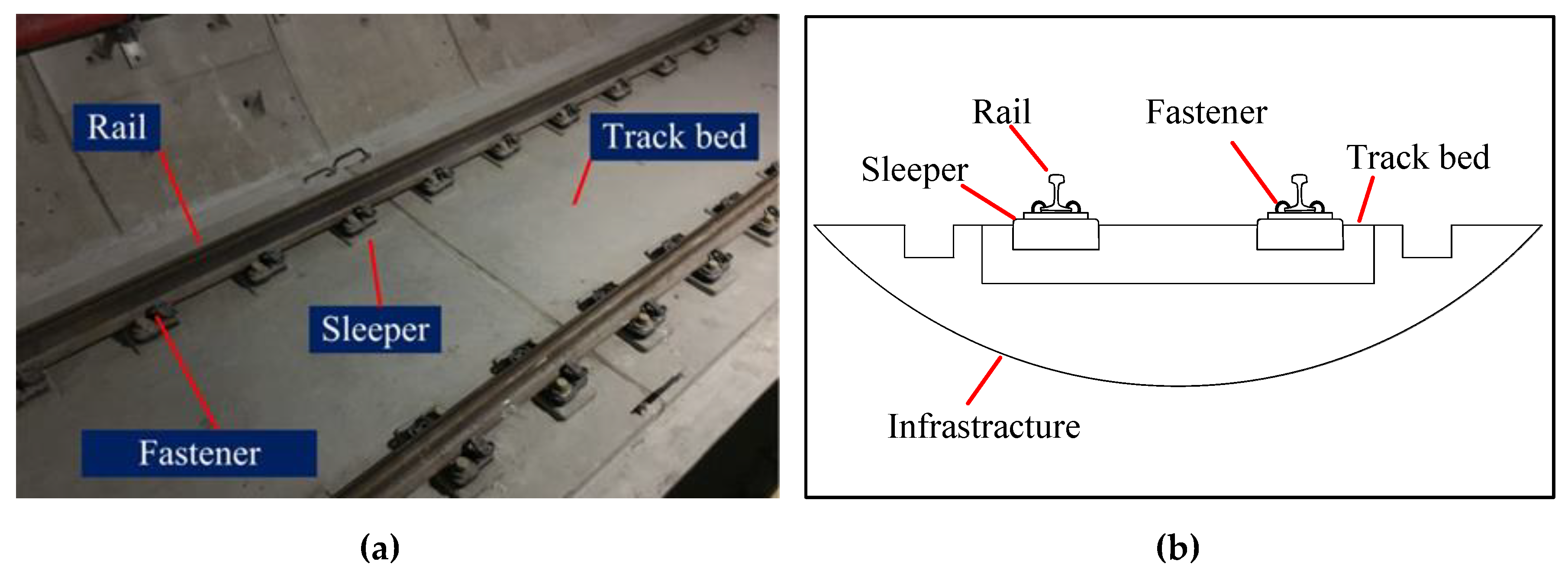
2.1.1. Monolithic Track Bed Structure

The monolithic track bed is the most common track structure of subways in China, which is investigated in this paper. It is comprised of CHN60 rails, fasteners, sleepers, the track bed and the infrastructure, as shown in Figure 1. The rail is mounted on sleepers by fasteners. Because the track bed connects the sleepers and the infrastructure rigidly, the sleepers, the track bed and the infrastructure can be considered as a whole. The vertical fastener stiffness of subway lines in China is generally less than 50 kN/mm [17].

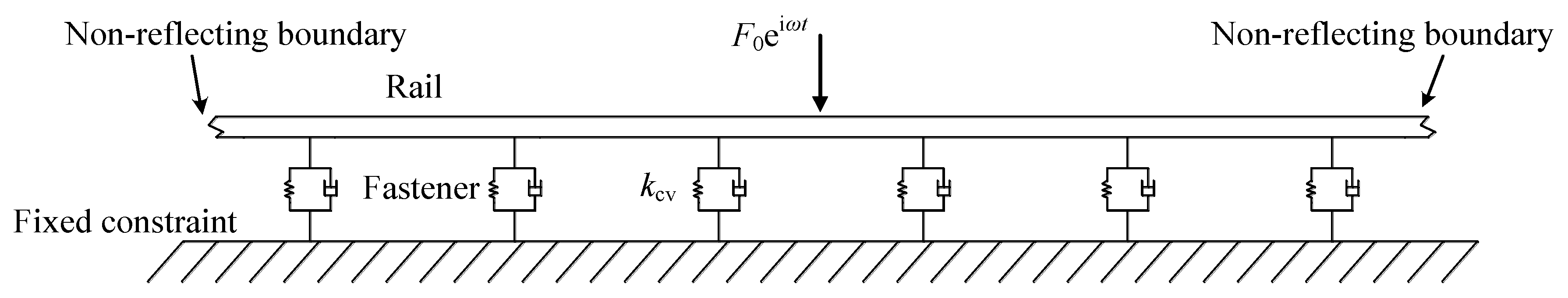
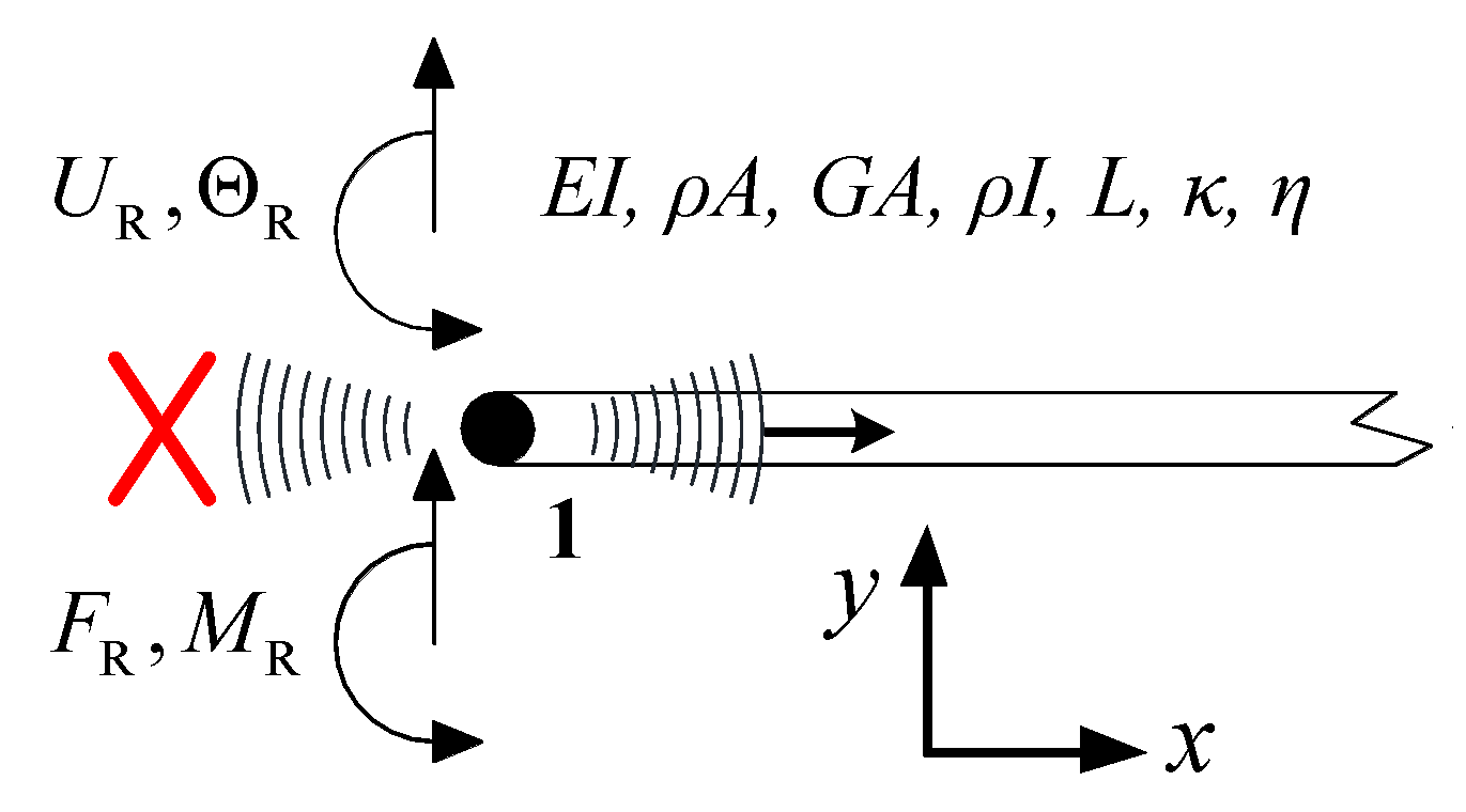
2.1.2. Timoshenko-Beam Track Model

To investigate the rail mobility/receptance, a Timoshenko-beam track model is established based on the structural properties of the monolithic track bed, as shown in Figure 2.

The model includes a long straight rail and fasteners. The sleepers, the track bed and the infrastructure are all considered as the fixed constraint. The rail is considered as a Timoshenko beam. As the cross-sectional deformation of the rail cannot be considered, the model is limited to frequencies of 1500 Hz [18]. To reduce the influence of the wave reflections, the non-reflecting boundary conditions are applied at both ends of the rail. In this way, the length of the model can also be shortened. The fastener is considered as a vertical extension spring whose upper end is connected to the rail beam and lower end is fixed. The fastener spacing (denoted by a) is obtained from the field measurement. To consider the damping of the fasteners, the complex vertical fastener stiffness k_cv is adopted for the vertical extension spring:

$$k_{\mathrm{cv}}=k_{\mathrm{v}}(1+i{\eta }_{\mathrm{f}})$$

(1)

where k_v is the vertical fastener stiffness and η_f is the damping loss factor of the fastener. A vertical harmonic point excitation F_v=F₀e^iωt is applied on the rail at the middle of the model, where F₀ is the amplitude, ω is the angular frequency, and t is the time.

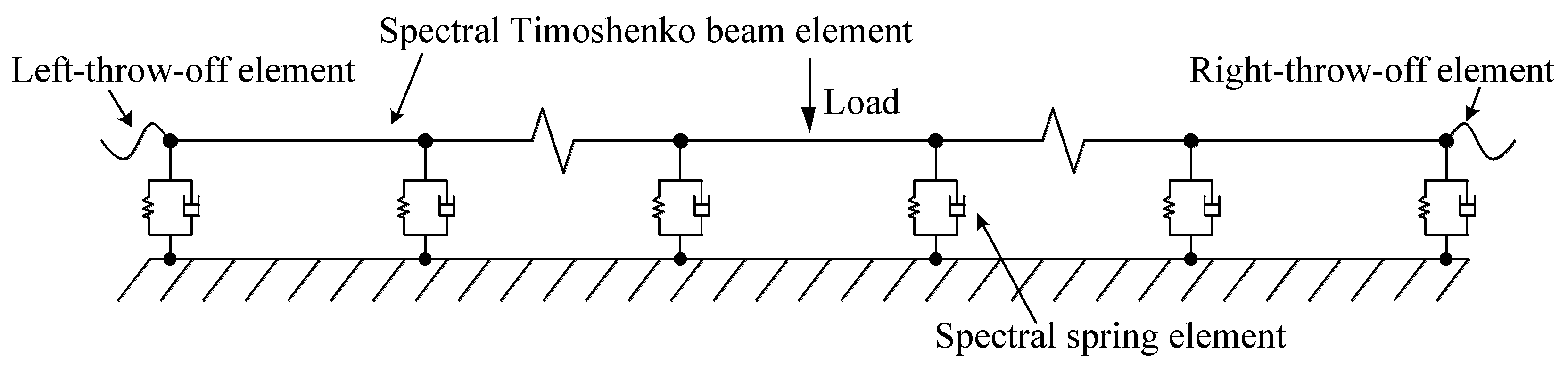
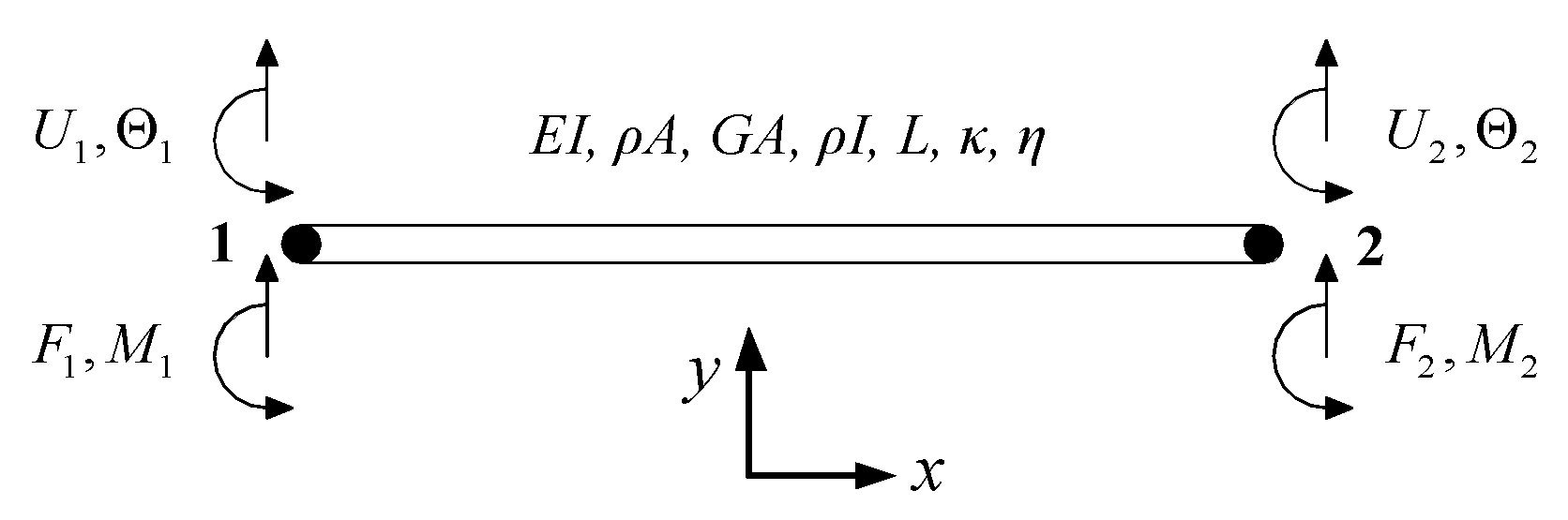
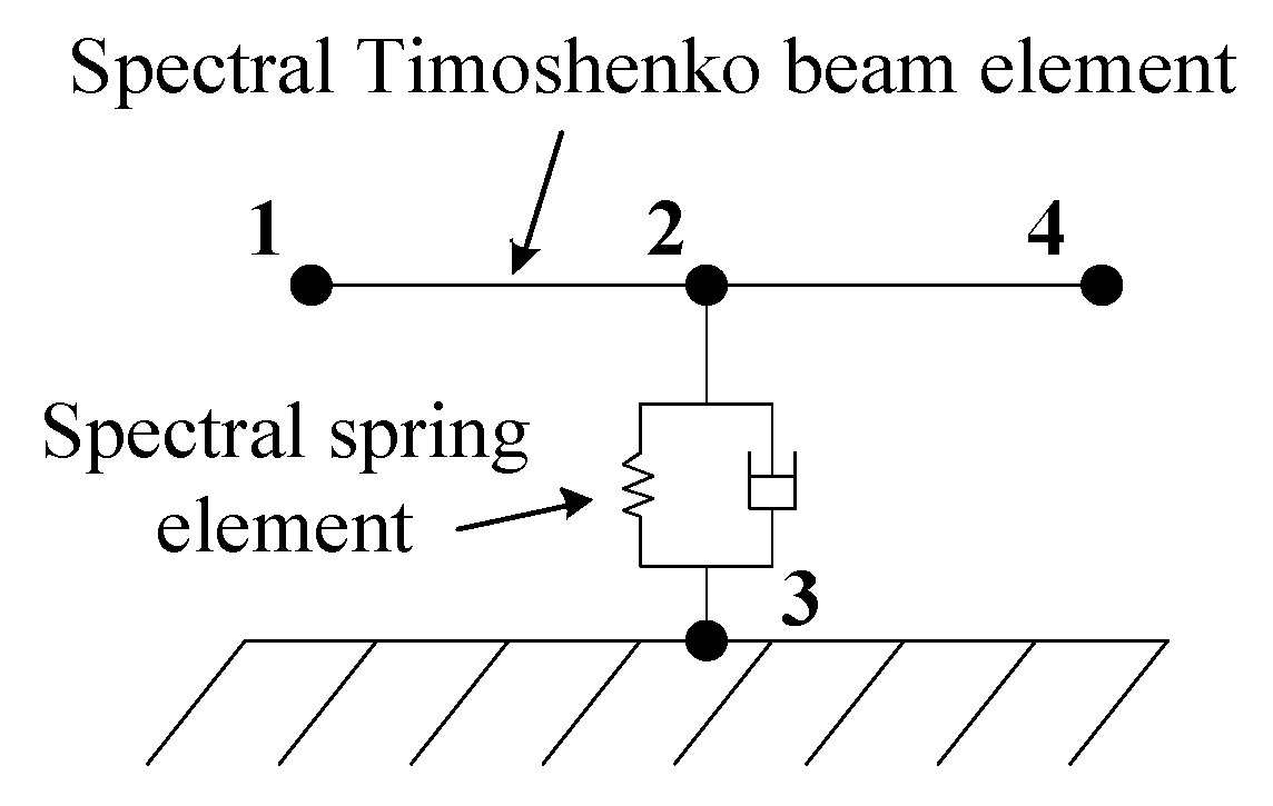
2.1.3. Spectral Element Method

The SEM is used to solve the Timoshenko-beam track model. As the spectral element size has no influence on the calculation precision of the SEM, the rail between two adjacent fasteners can be modeled as only one spectral Timoshenko beam element. To simulate the non-reflecting boundary conditions, two Timoshenko beam throw-off elements are modeled at two ends of the long rail. The vertical extension spring is modeled with a two-node spectral spring element. The element division is shown in Figure 3 where the black dots represent the nodes.

The two-node spectral Timoshenko beam element is shown in Figure 4.

E is the Young’s modulus, I is the area moment of inertia, ρ is the mass density, A is the cross-sectional area, G is the shear modulus, L is the length of the spectral element, κ is the shear correction factor and η is the damping loss factor. U₁, Θ₁, F₁ and M₁ are the spectral vertical displacement, spectral bending rotation, spectral vertical force and spectral bending moment at the left node, respectively, while U₂, Θ₂, F₂ and M₂ are the corresponding items at the right node. The relation between the spectral nodal displacements and the spectral nodal forces in a spectral Timoshenko beam element can be expressed as:

$${\mathbf{F}}_{\mathbf{t}}={\mathbf{S}}_{\mathbf{t}}(\omega ){\mathbf{U}}_{\mathbf{t}}$$

(2)

where F_t = (F₁, M₁, F₂, M₂)^T is the spectral nodal force vector, U_t = (U₁, Θ₁, U₂, Θ₂)^T is the spectral nodal displacement vector, S_t(ω) is the frequency-dependent spectral element stiffness matrix, and ω is the angular frequency. The derivation of Equation (2) is based on the free vibration of a uniform Timoshenko beam and the spectral analysis. The spectral element stiffness matrix S_t(ω) is obtained by substituting the wave solution into the governing differential equations. The expression of S_t(ω) can be given by:

$${\mathbf{S}}_{\mathbf{t}}(\omega )=\left(\begin{array}{c}EI{\mathbf{N}}^{″}(0,\omega )+\rho I{\omega }^2\mathbf{N}(0,\omega )\\ -EI{\widehat{\mathbf{N}}}^{\prime }(0,\omega )\\ -EI{\mathbf{N}}^{″}(L,\omega )-\rho I{\omega }^2\mathbf{N}(L,\omega )\\ EI{\mathbf{N}}^{\prime }(L,\omega )\end{array}\right)\left(\begin{array}{cccc}(r_1+r_2{e}_2)& -R_2(r_1-r_2{e}_2)& -(r_1{e}_2+r_2)& R_2(r_1{e}_2-r_2)\\ -(r_1+r_2{e}_1)& R_1(r_1-r_2{e}_1)& (r_1{e}_1+r_2)& -R_1(r_1{e}_1-r_2)\\ (r_1{e}_2+r_2)& R_2(r_1{e}_2-r_2)& -(r_1+r_2{e}_2)& -R_2(r_1-r_2{e}_2)\\ -(r_1{e}_1+r_2)& -R_1(r_1{e}_1-r_2)& (r_1+r_2{e}_1)& R_1(r_1-r_2{e}_1)\end{array}\right)\frac{1}{\mathsf{\Delta }}$$

(3)

$$\mathbf{N}(x,\omega )=(\begin{array}{cccc}{\mathrm{e}}^{-\mathrm{i}{k}_{1}x}& {\mathrm{e}}^{-\mathrm{i}{k}_{2}x}& {\mathrm{e}}^{-\mathrm{i}{k}_1(L-x)}& {\mathrm{e}}^{-\mathrm{i}{k}_2(L-x)}\end{array})$$

(4)

$$k_1=\sqrt{\frac{a_1}{2}+\sqrt{\frac{a_1^2}{4}-a_2}},\hspace{1em}{k}_2=\sqrt{\frac{a_1}{2}-\sqrt{\frac{a_1^2}{4}-a_2}}$$

(5)

$$a_1=\frac{GA\kappa \rho I{\omega }^2+EI\rho A{\omega }^2}{GA\kappa EI},\hspace{1em}{a}_2=\frac{\rho A{\omega }^2(\rho I{\omega }^2-GA\kappa )}{GA\kappa EI}$$

(6)

$$R_m=\frac{\mathrm{i}GA\kappa k_m}{GA\kappa k_m^2-\rho A{\omega }^2}\hspace{1em}(m=1,2)$$

(7)

$$r_1=(R_1-R_2)(1-e_1{e}_2),\hspace{1em}{r}_2=(R_1+R_2)(e_1-e_2),\hspace{1em}{e}_1={\mathrm{e}}^{-\mathrm{i}{k}_{1}L},\hspace{1em}{e}_2={\mathrm{e}}^{-\mathrm{i}{k}_{2}L},\hspace{1em}\mathsf{\Delta }=r_1^2-r_2^2$$

(8)

where k₁ and k₂ are the wavenumbers. The derivation of S_t(ω) has been demonstrated in the previous work [16], which is omitted in this paper. F_t is the input determined by the external loads.

In order to simulate the non-reflecting boundary conditions, the Timoshenko beam throw-off elements are modeled at both ends of the rail. The reflected waves can be prohibited by removing the reflection items in the wave solutions of the Timoshenko beam. The one-node Timoshenko beam right-throw-off element which prevents the reflecting waves from travelling to the left is shown in Figure 5.

U_R, Θ_R, F_R and M_R are the spectral vertical displacement, spectral bending rotation, spectral vertical force and spectral bending moment at the node, respectively. Similarly, the relation between the spectral nodal displacements and the spectral nodal forces in a Timoshenko beam right-throw-off element can be expressed as:

$${\mathbf{F}}_{\mathbf{R}}={\mathbf{S}}_{\mathbf{R}}(\omega ){\mathbf{U}}_{\mathbf{R}}$$

(9)

where F_R = (F_R, M_R)^T is the spectral nodal force vector, U_R = (U_R, Θ_R)^T is the spectral nodal displacement vector, and S_R(ω) is the frequency-dependent spectral element stiffness matrix. The expression of S_R(ω) can be given by:

$${\mathbf{S}}_{\mathbf{R}}=\left(\begin{array}{cc}EI\frac{k_2^2-k_1^2}{R_1-R_2}& EI\frac{R_2{k}_1^2-R_1{k}_2^2}{R_1-R_2}+{\omega }^2\rho I\\ EI\frac{\mathrm{i}(k_1-k_2)}{R_1-R_2}& EI\frac{\mathrm{i}(R_1{k}_2-R_2{k}_1)}{R_1-R_2}\end{array}\right)$$

(10)

The derivation of S_R (ω) is omitted as in the case of Equation (2). Because the derivations of the spectral element stiffness matrixes of the spectral spring element and the Timoshenko beam left-throw-off element follow the same pattern, these spectral elements are not represented for the purpose of conciseness.

Using the coordinate transformation approach, the spectral element stiffness matrix in the local coordinate system can be transformed for the global coordinate system. The spectral stiffness matrix of the whole model can be obtained by assembling the spectral element stiffness matrixes and processing the constraint conditions, which is same as the conventional finite element method. The relation between the spectral nodal displacements and the spectral nodal forces for the whole model can be expressed as:

$$\mathbf{F}=\mathbf{S}(\omega )\mathbf{U}$$

(11)

where F is spectral nodal force vector of the whole model, U is the spectral nodal displacement vector, and S(ω) is the spectral stiffness matrix. By solving Equation (11), we can obtain the frequency-domain dynamic characteristics of rail vibrations in the Timoshenko-beam track model. For a static and linear system, the amplitude of the mobility is 2πf times that of the receptance at the frequency f, while the amplitude of the accelerance is 2πf times that of the mobility. Based on this knowledge, the rail mobility/accelerance can be obtained by the simple post processing.

2.2. Model and Method for the Decay Rate

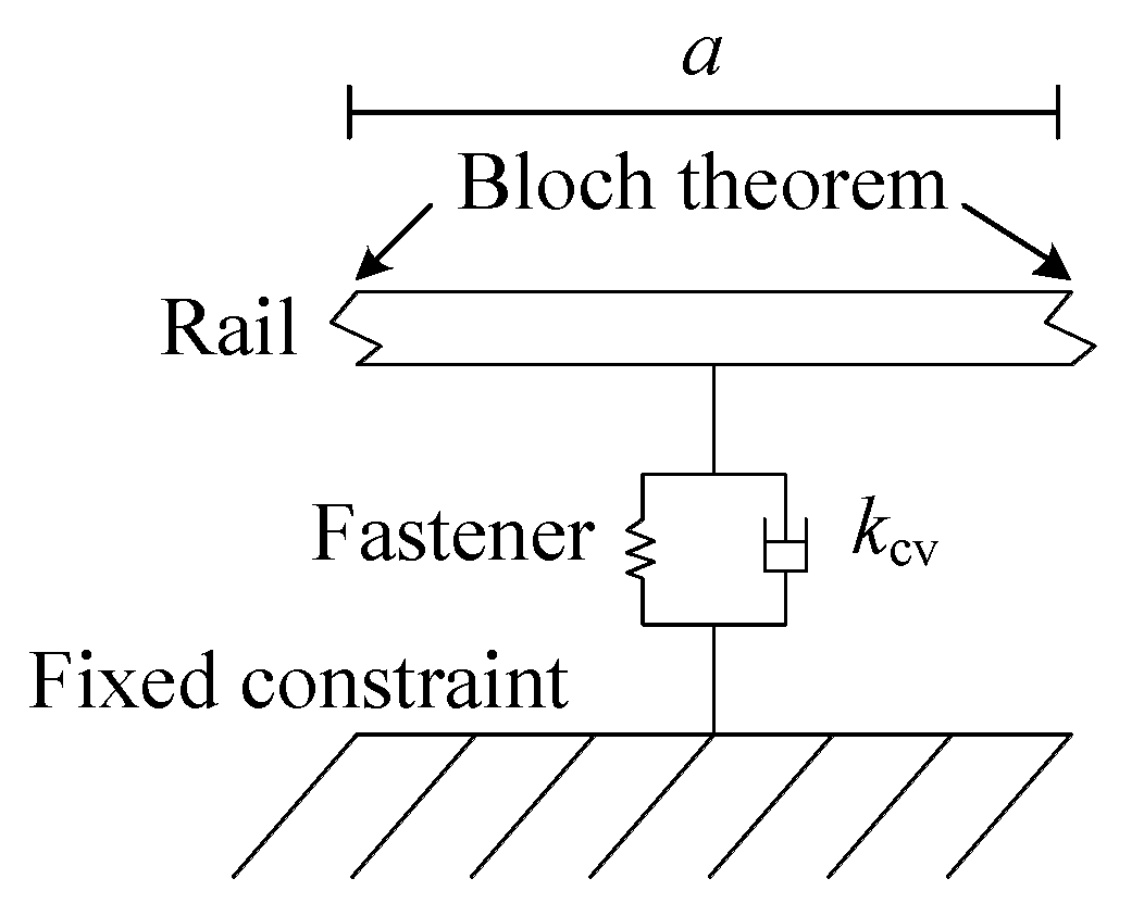
2.2.1. Periodic Track Model

To investigate the DR, a periodic track model is established, as shown in Figure 6. The length of the model equals to the fastener spacing a. The modeling ways of track components are the same as those in the Timoshenko-beam track model. As the monolithic track bed can be considered as the one-dimensional periodic structure, the Bloch theorem for the periodic structure is applied at both ends of the rail.

2.2.2. Spectral Transfer Matrix Method

The STMM is used to solve the periodic track model. The short rail is divided into two spectral Timoshenko beam elements. The vertical extension spring representing the fastener is modeled with a two-node spectral spring elements. The model has 4 nodes and 3 spectral elements in total. The element division is shown in Figure 7.

The spectral stiffness matrix of the periodic track model can be obtained by using the SEM. Thus, the relation between the spectral nodal forces and displacements of the periodic track model can be expressed as:

$$\left[\begin{array}{cccc}{\mathbf{S}}_{\mathbf{11}}& {\mathbf{S}}_{\mathbf{12}}& {\mathbf{S}}_{\mathbf{13}}& {\mathbf{S}}_{\mathbf{14}}\\ {\mathbf{S}}_{\mathbf{21}}& {\mathbf{S}}_{\mathbf{22}}& {\mathbf{S}}_{\mathbf{23}}& {\mathbf{S}}_{\mathbf{24}}\\ {\mathbf{S}}_{\mathbf{31}}& {\mathbf{S}}_{\mathbf{32}}& {\mathbf{S}}_{\mathbf{33}}& {\mathbf{S}}_{\mathbf{34}}\\ {\mathbf{S}}_{\mathbf{41}}& {\mathbf{S}}_{\mathbf{42}}& {\mathbf{S}}_{\mathbf{43}}& {\mathbf{S}}_{\mathbf{44}}\end{array}\right]\left(\begin{array}{c}{\mathbf{U}}_{\mathbf{1}}\\ {\mathbf{U}}_{\mathbf{2}}\\ {\mathbf{U}}_{\mathbf{3}}\\ {\mathbf{U}}_{\mathbf{4}}\end{array}\right)=\left(\begin{array}{c}{\mathbf{F}}_{\mathbf{1}}\\ {\mathbf{F}}_{\mathbf{2}}\\ {\mathbf{F}}_{\mathbf{3}}\\ {\mathbf{F}}_{\mathbf{4}}\end{array}\right)$$

(12)

where U_i is the spectral nodal displacement vector of node i (i = 1–4), and F_j is the spectral nodal force vector of node j (j = 1–4). The spectral stiffness matrix of the model is divided into a 4 × 4 partitioned matrix according to the node number, while the submatrix is denoted by S_ij. To build the transfer relation between the left and right ends, the matrix in Equation (12) is partitioned again, as shown in the following:

$$\left(\begin{array}{ccc}{\mathbf{S}}_{1L}& {\mathbf{S}}_{1M}& {\mathbf{S}}_{1R}\\ {\mathbf{S}}_{2L}& {\mathbf{S}}_{2M}& {\mathbf{S}}_{2R}\\ {\mathbf{S}}_{3L}& {\mathbf{S}}_{3M}& {\mathbf{S}}_{3R}\end{array}\right)\left(\begin{array}{c}{\mathbf{U}}_{\mathbf{L}}\\ {\mathbf{U}}_{\mathbf{M}}\\ {\mathbf{U}}_{\mathbf{R}}\end{array}\right)=\left(\begin{array}{c}{\mathbf{F}}_{\mathbf{L}}\\ {\mathbf{F}}_{\mathbf{M}}\\ {\mathbf{F}}_{\mathbf{R}}\end{array}\right)$$

(13)

where

$$\begin{array}{l}{S}_{1L}=S_{11}, S_{1M}=\left(\begin{array}{cc}{S}_{12}& S_{13}\end{array}\right), S_{1R}=S_{14},\\ S_{2L}={\left(\begin{array}{cc}{S}_{21}& S_{31}\end{array}\right)}^T, S_{2M}=\left(\begin{array}{cc}{S}_{22}& S_{23}\\ S_{32}& S_{33}\end{array}\right), S_{2R}={\left(\begin{array}{cc}{S}_{24}& S_{34}\end{array}\right)}^T,\\ S_{3L}=S_{41}, S_{3M}=\left(\begin{array}{cc}{S}_{42}& S_{43}\end{array}\right), S_{3R}=S_{44},\\ U_L=U_1, U_M={\left(\begin{array}{cc}{U}_2& U_3\end{array}\right)}^T, U_R=U_4,\\ F_L=F_1, F_M={\left(\begin{array}{cc}{F}_2& F_3\end{array}\right)}^T, F_R=F_4,\end{array}$$

(14)

As nodes 2 and 3 are not subjected to any external loads in the transfer relation, i.e., F_M = 0, the following can be obtained from Equation (13):

$$T\left(\begin{array}{c}{U}_L\\ U_R\end{array}\right)=\left(\begin{array}{c}-F_L\\ F_R\end{array}\right)$$

(15)

where

$$T=\left[\begin{array}{cc}{T}_{11}& T_{12}\\ T_{21}& T_{22}\end{array}\right]=\left[\begin{array}{cc}-S_{1L}+S_{1M}{S}_{2M}^{-1}{S}_{2L}& -S_{1R}+S_{1M}{S}_{2M}^{-1}{S}_{2R}\\ S_{3L}-S_{3M}{S}_{2M}^{-1}{S}_{2L}& S_{3R}-S_{3M}{S}_{2M}^{-1}{S}_{2R}\end{array}\right]$$

(16)

Equation (15) may be expressed in the form of the transfer relation between two ends:

$$\left(\begin{array}{c}{U}_R\\ F_R\end{array}\right)=t(\omega )\left(\begin{array}{c}{U}_L\\ -F_L\end{array}\right)$$

(17)

where t(ω) is the spectral transfer matrix:

$$t(\omega )=\left[\begin{array}{cc}-T_{12}^{-1}{T}_{11}& T_{12}^{-1}\\ T_{21}-T_{22}{T}_{12}^{-1}{T}_{11}& T_{22}{T}_{12}^{-1}\end{array}\right]$$

(18)

The following can be obtained using the Bloch theorem [19]:

$$\left(\begin{array}{c}{U}_R\\ F_R\end{array}\right)={\mathrm{e}}^{-\mathrm{i}{k}_{\mathrm{x}}a}\left(\begin{array}{c}{U}_L\\ -F_L\end{array}\right)$$

(19)

where k_x is the one-dimensional Bloch wave vector, i.e., the wavenumber. A standard eigenvalue problem of the 4 × 4 matrix can be obtained by combining Equations (17) and (19):

$$\left|t-{\mathrm{e}}^{-\mathrm{i}{k}_{\mathrm{x}}a}I\right|=0$$

(20)

The dispersion relation between the wavenumber k_x and the angular frequency ω can be obtained by solving the eigenvalue problem. For the bending motion of the Timoshenko beam, the solutions of the wavenumbers appear in pairs of opposite sign (±k_x), describing two waves propagating in opposite directions. As the eigenvalue problem is represented by a 4 × 4 matrix, the solution contains two pairs of Bloch waves for the periodic track model. Furthermore, the DR can be obtained according to [20]:

$$DR=-8.686\mathrm{Im}(k_x)$$

(21)

where Im(k_x) is the imaginary part of k_x. The parameters of the Timoshenko-beam track model and the periodic track model are listed in

Table 1. Parameters of models.

Track component	Parameter	Symbol	Value
CHN60 rail	Elastic modulus (GPa)	E	210
	Cross-section area (m2)	A	7.745 × 10−3
	Mass density (kg/m3)	ρ	7850
	Shear correction factor	κ	0.5329
	Area moment of inertia (m4)	I	3.217 × 10−5
	Damping loss factor	ηr	0.05
	Shear elastic modulus (GPa)	G	80.77
Fastener	Vertical stiffness (kN/mm)	kv	37
	Damping loss factor	ηf	0.25
	Spacing (m)	a	0.625

. The vertical fastener stiffness k_v is obtained by fitting simulations to field measurements.

2.3. Calculation of Rail Sound Power Level

The sound power level L_w of an infinite rail can be expressed as [2]:

$$L_{\mathrm{w}}\approx 101\mathrm{g}(\frac{4.343{\rho }_0{c}_0\sigma P}{2W_0})+201\mathrm{g}\left|v(0)\right|-101\mathrm{g}DR$$

(22)

where W₀=10⁻¹² W is the reference of the sound power, v(0) is the velocity amplitude of the rail at x = 0, ρ₀ = 1.225 kg/m³ is the air density, c₀ = 340 m/s is the propagation velocity of sound waves in air, σ is the radiation ratio, and P is the length that the cross-section perimeter projected onto a plane perpendicular to the motion (P = 0.413 m for vertical rail vibrations). The radiation ratio σ is given from the reference [2], which is calculated by using a rail above a rigid ground surface.

Equation (22) indicates that the increase of the velocity amplitude at x = 0 and the decrease of the DR will both lead to the increase of the rail sound power level. By substituting the calculation results of the rail mobility amplitude and the DR into Equation (22), the sound power level of the rail subjected to a harmonic point excitation can be obtained.

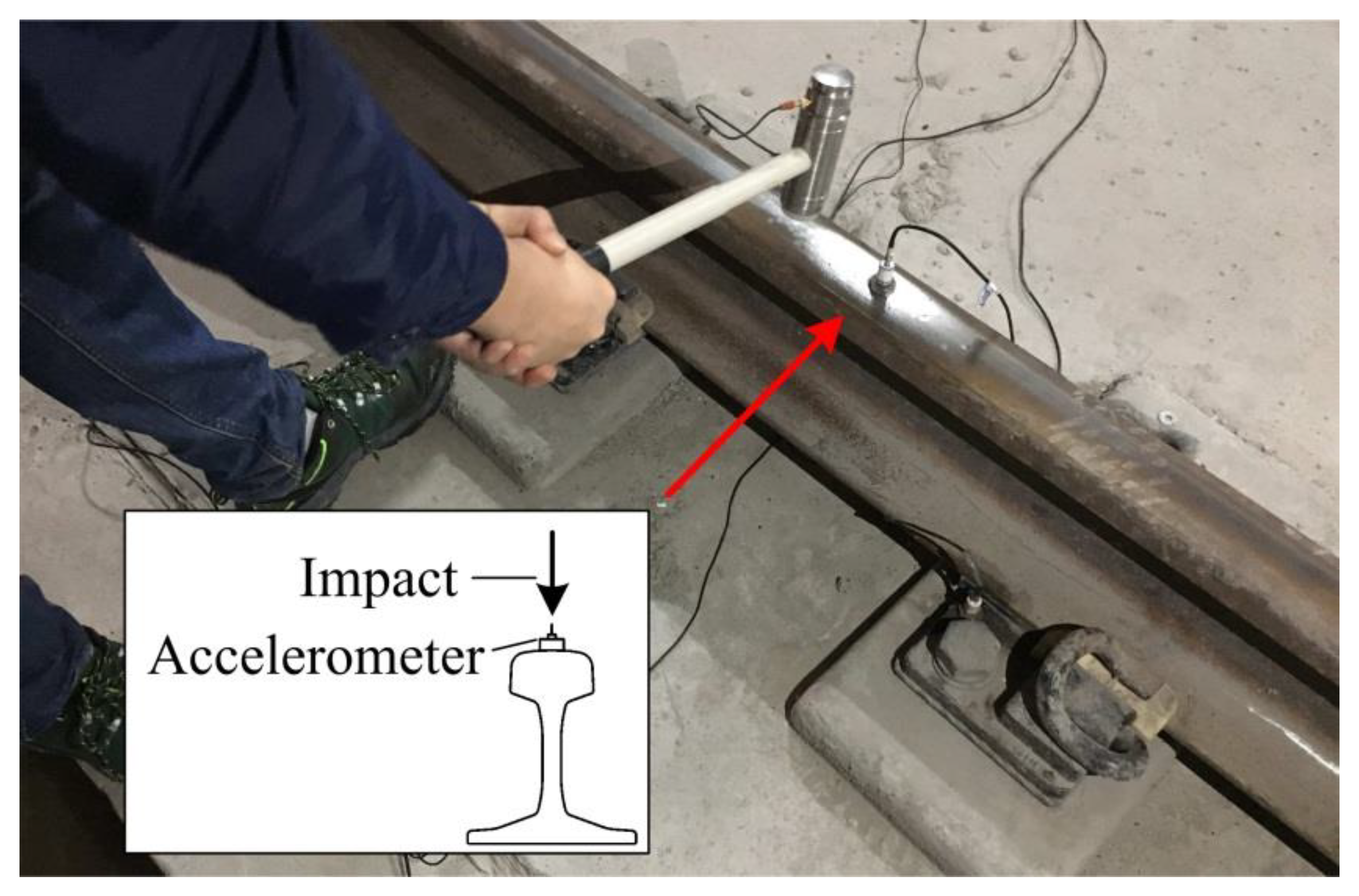
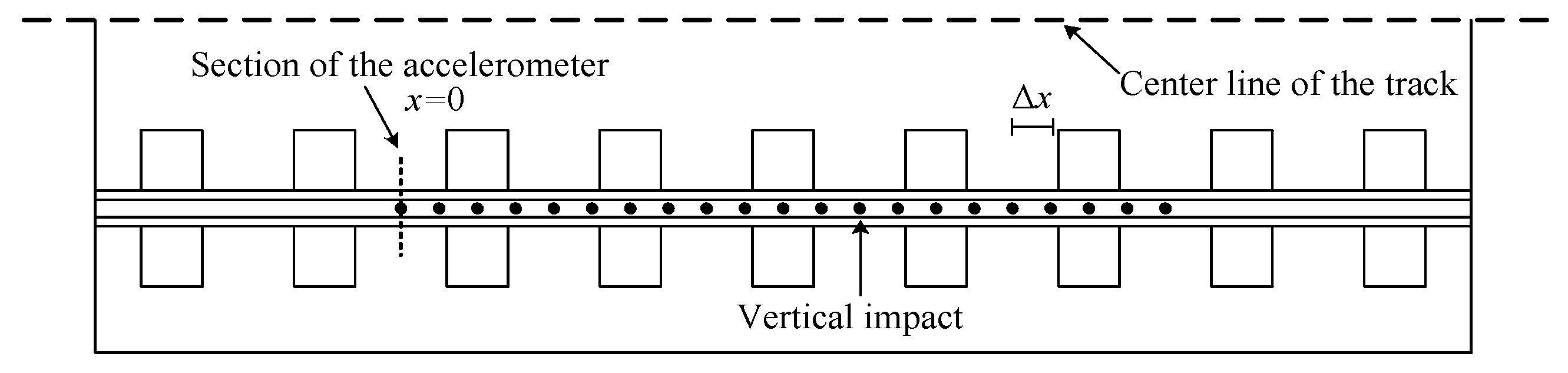
3. Field Measurement

Field measurements were carried out to verify the accuracy of models and methods in this paper. The measurements were conducted in an existing subway line in China, where the track structure type is the straight monolithic track bed. It consists of CHN60 rails, GJ-III fasteners, sleepers, the track bed and the infrastructure. The measurement section was far from the turnout and the rail joints. The track was in good condition, and the fastener spacing was 0.625 m.

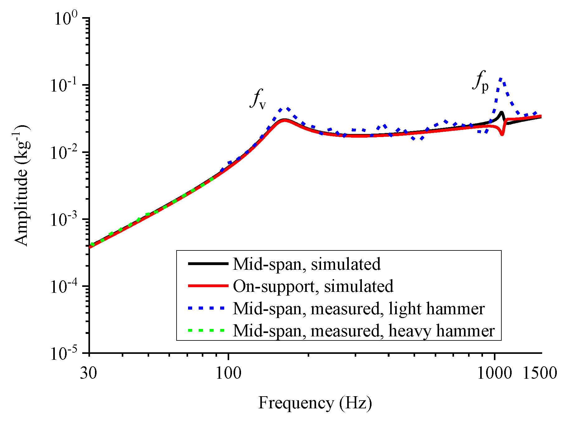
3.1. Rail Accelerance

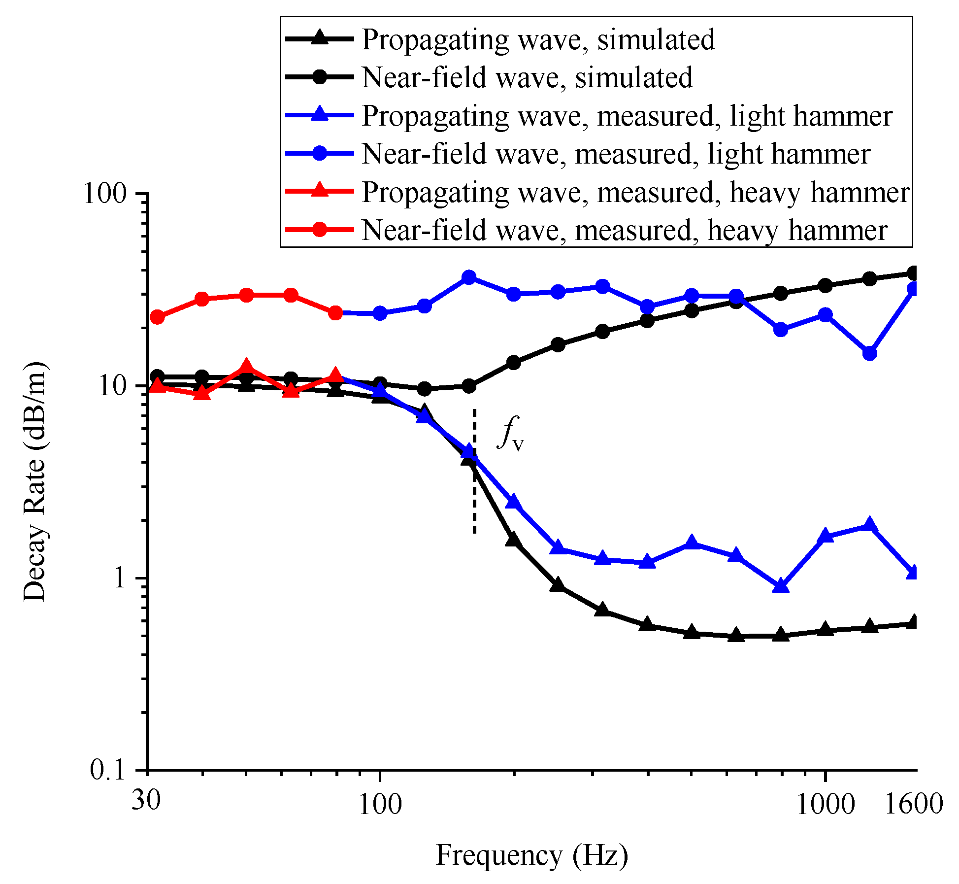
The rail accelerance was measured for the purpose of verifying the accuracy of the Timoshenko-beam track model and the SEM. An accelerometer was placed on the mid-span railhead, and then a hammer was used to impact the same position. The direct vertical accelerance of the mid-span rail was obtained by processing the signals of the accelerometer and the hammer. The field measurement is shown in Figure 8.

The operating frequency range, the nominal sensitivity, and the measurement range of the accelerometer were 1–15,000 Hz, 5 mV/g, and 1000 g, respectively. As distinct hammers have different applicable frequency ranges, a heavy hammer with a nylon head was used to acquire the low-frequency measurement result, while a light hammer with an aluminum head was used to acquire the middle- and high-frequency measurement result. The lower boundary of the applicable frequency range depends on the coherent coefficient of the rail accelerance. It should exceed 0.8 within the applicable frequency range [21]. The upper boundary of the applicable frequency range should meet the requirement that the decrease of the amplitude spectrum of the impact force is less than 10 dB when the amplitude at low frequencies is taken as the reference [22]. Based on these rules, the applicable frequency ranges of the heavy and light hammers were 25–600 Hz and 90–3900 Hz, respectively. The sampling frequency of the acquisition instrument was 3200 Hz when the heavy hammer was used, and it was changed to 25,600 Hz when the light hammer was used. Besides, the measurement ranges of the heavy and light hammers were 125 kN and 50 kN, respectively.

To eliminate the measurement errors induced by the noises, five effective impacts were required in the measurement, and the average of the results was taken as the final result. The final measurement result of the rail accelerance is comprised of two parts: the result obtained by the heavy hammer for the frequency range of 30–90 Hz and the result obtained by the light hammer for the frequency range of 90–2000 Hz.

3.2. Decay Rate

The standard EN15461: 2008+A1: 2010 [23] presents a general measurement method of the DR. However, this method does not perform the experimental wavenumber decomposition, as a result of which only one DR curve encompassing the attenuation behaviors of all waves is obtained. In order to obtain the separate DR of each wave, the experimental analysis method of wave propagation in the reference [24] was adopted for the DR measurement. After placing an accelerometer on the mid-span railhead, a number of hammer impacts were applied on the railhead in the longitudinal direction at equal intervals of Δx = 0.625/4 m = 0.15625 m. The number of impact points was Q = 21. The positions of the accelerometer and hammer impacts are shown in Figure 9.

The rail accelerance h(x) at the position x= (q-1)Δx, where q = 1, 2, …, Q, was obtained by processing the signals of the accelerometer and the hammer. At each frequency, the rail accelerance h(x) can be approximated as a sum of N waves:

$$h(x)=h((q-1)\mathsf{\Delta }x)\approx {\displaystyle \sum _{n=1}^N{A}_n{\mathrm{e}}^{s_n(q-1)\mathsf{\Delta }x}}$$

(23)

where s_n = -β_n-ik_n is the complex propagation coefficient, β_n is the decay coefficient, k_n is the wavenumber, and A_n is the complex amplitude. The Prony method [25] was used to solve the Equation (23). After obtaining the unknown s_n, we calculated the DR of each wave according to:

$$D{R}_n=-201\mathrm{g}\left|{\mathrm{e}}^{s_n}\right|=8.686{\beta }_n$$

(24)

In order to make a better comparison between the measurement and the simulation, let N be given by 2. Therefore, the results of the simulation and measurement each include two DR curves corresponding to two different waves. As same with the measurement of the rail accelerance, the result of the DR is comprised of two parts: the result obtained by the heavy hammer for the frequency range of 30–90 Hz and the result obtained by the light hammer for the frequency range of 90–2000 Hz.

4. Results

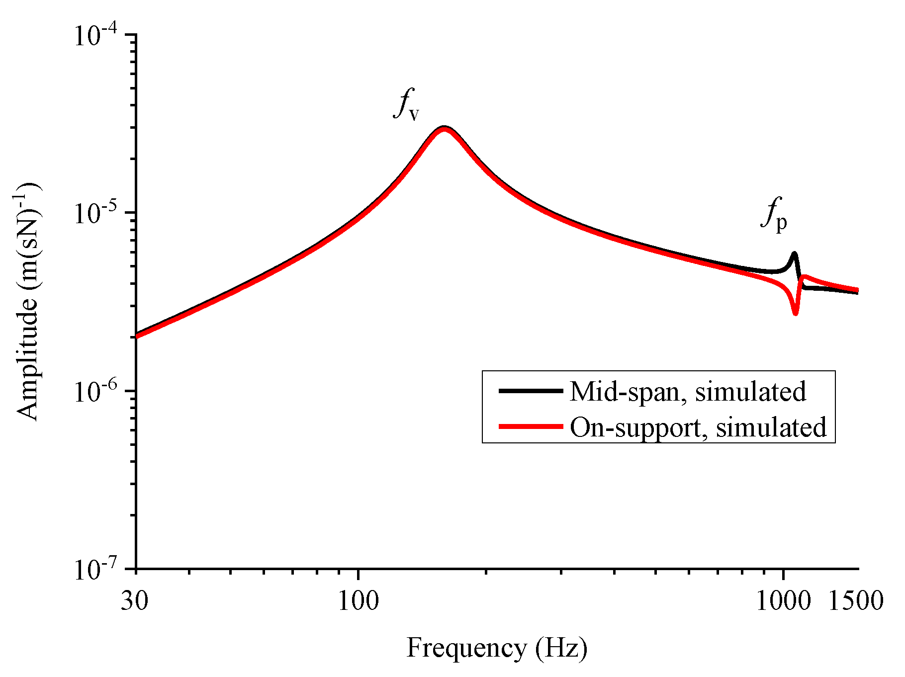
4.1. Rail Accelerance and Mobility

The rail accelerance and mobility are helpful to the investigation of vibration characteristics, which are of great importance to explain the rail sound power characteristics. The amplitudes of the direct vertical rail accelerance and mobility are shown in Figure 10 and Figure 11, respectively.

According to Figure 10, the simulated amplitude of the direct mid-span rail accelerance increases with the increase of the frequency in the low-frequency range and reaches the peak at 163 Hz where the vertical rail resonance occurs. The resonance frequency is denoted by f_v, and it depends on the vertical fastener stiffness. In the frequency range of 200–1000 Hz, the accelerance amplitude does not change much. Another peak appears at 1063 Hz where the first-order vertical pinned–pinned rail resonance occurs. This resonance frequency is denoted by f_p. The corresponding modal shape turns out to be a standing wave with nodes at the fastener, and the half-wavelength equals to the fastener spacing. The on-support and mid-span rail accelerance amplitude curves coincide with each other besides the parts near f_p. As the nodes of the standing wave are located at the fasteners, there is a trough at f_p in the on-support rail accelerance amplitude curve.

Due to the vertical rail resonance and the first-order vertical pinned–pinned rail resonance, there are also two peaks at f_v and f_p in the direct mid-span rail mobility amplitude curve. However, the rail mobility amplitude decreases with the increase of the frequency above f_v, which is different from the accelerance amplitude curve. The on-support and mid-span rail mobility amplitude curves also coincide with each other besides the parts near f_p.

The measurement and the simulation of the mid-span rail accelerance amplitude match well. The peaks at f_v and f_p are obvious in the measured accelerance amplitude curve. Therefore, the Timoshenko-beam track model and the SEM are adequate for studying the rail vibration characteristics of the monolithic track bed structure.

4.2. Decay Rate

The DR controls the effective radiating length of the rail. The simulation and the measurement of the DRs are shown in Figure 12, which is presented in the form of one-third octave spectra.

Figure 12 shows that the DRs of two waves are quite different. The first wave (marked by the circles) holds a high DR at all frequencies, which is called the near-field wave. The second wave (marked by the triangles) only has a high DR in the low-frequency range, which is called the propagating wave. As the near-field wave is attenuated significantly, the transmission characteristics of the rail vibrations in the longitudinal direction is mainly determined by the propagating wave. Thus, this paper primarily investigates the DR of the propagating wave.

According to the simulation result, the vertical rail resonance does not occur below f_v. Consequently, the propagating wave cannot propagate freely, and the DR of the propagating wave keeps a high value. Below the center frequency of 100 Hz, the DR is more than 8 dB/m. The DR starts decreasing quickly near the frequency of f_v. Thus, the vertical rail resonance frequency f_v is the boundary frequency of the high DR band. Then, the DR decreases with the increase of frequency. It is only about 0.5 dB/m at the center frequency of 1000 Hz. The DR in the low-frequency range is higher than that in the high-frequency range, so the vertical rail vibrations in the low-frequency range are mainly transmitted in the downward direction while those at high frequencies are primarily transmitted along the rail.

The measurement and the simulation of the DR of the propagating wave match well. Below the center frequency of 160 Hz, they coincide with each other. In the high-frequency range, the measured DR keeps the low values as the simulated DR does. Therefore, the periodic track model and the STMM are adequate for studying the attenuation characteristics of rail vibrations in the longwise direction.

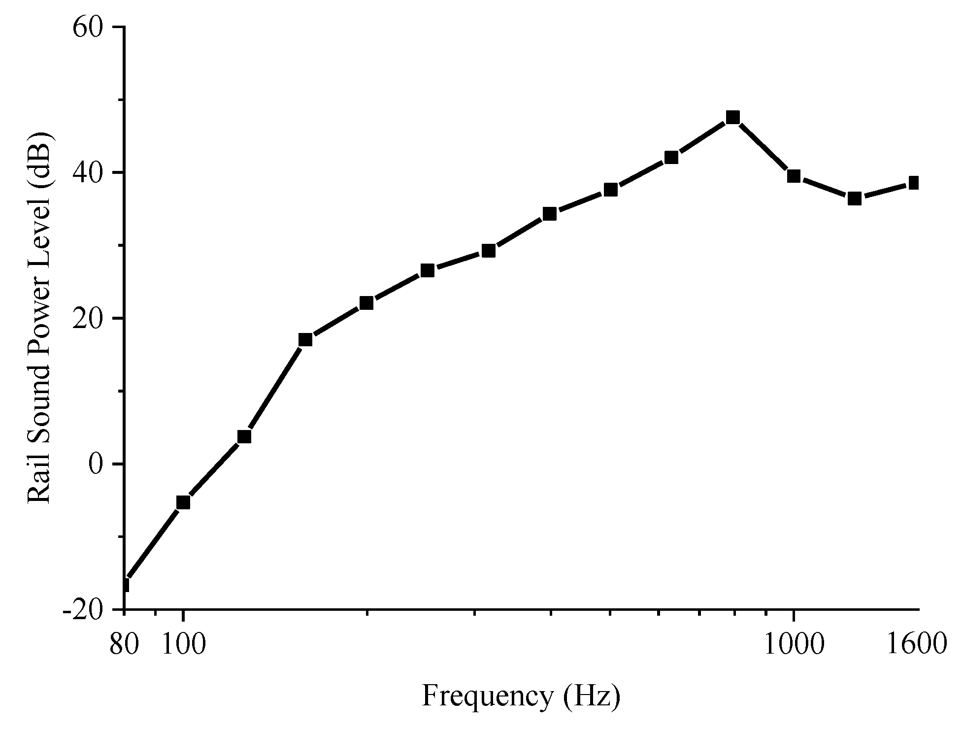
4.3. Rail Sound Power Level

By substituting the calculation results of the rail mobility amplitude (Figure 11) and the DR (Figure 12) into Equation (22), the sound power level of the rail subjected to a harmonic point excitation can be obtained, as shown in Figure 13 (in the form of the one-third octave spectra).

Below the center frequency of 800 Hz, the rail sound power level increases with the increase of frequency. A peak appears at the center frequency of 800 Hz with the value of 48 dB. In the frequency range of 1000–1600 Hz, the rail sound power level is within the range of 36–39 dB.

The high rail mobility amplitude and the low DR will both lead to a significant rail sound power level. Figure 11 and Figure 12 show that although the direct mid-span rail mobility amplitude is significant near the frequency f_v, the DR also has a high value. As a result, no peak occurs in the curve of the rail sound power level near f_v. However, there is a peak at the center frequency of 800 Hz. As the DR and the mobility amplitude both decrease with the increase of frequency, the contributions of the second and the third items of Equation (22) to the rail sound power level are cancelled out by each other to a certain extent. Furthermore, the rail radiation ratio increases with the increase of frequency and reaches a peak near the center frequency of 800 Hz [2]. Thus, it is the main reason why the rail sound power level reaches a peak at the center frequency of 800 Hz.

5. Influence of the Vertical Fastener Stiffness

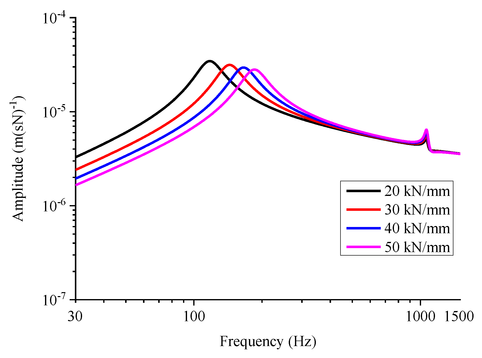
5.1. Influence on the Rail Mobility Amplitude

The simulated influence of the vertical fastener stiffness on the direct mid-span rail mobility amplitude is shown in Figure 14. The general vertical stiffness of the non-vibration-mitigation fasteners in subway lines is 30–40 kN/mm. The vertical stiffness of the vibration-mitigation fasteners can be 20 kN/mm.

When the vertical fastener stiffness varies within the range of 20–50 kN/mm, only the part below 400 Hz has the obvious changes of the vertical rail resonance frequency and the amplitudes. With the increase of the vertical fastener stiffness, the vertical rail resonance frequency f_v increases while the value of the peak decreases slightly. When the vertical rail resonance frequency increases from f_v to f_v^*, the mobility amplitude below f_v decreases while that above f_v^* increases. The maximal decrease and increase occur at f_v and f_v^*, respectively. The influence of vertical fastener stiffness on the amplitude is small in the high-frequency range.

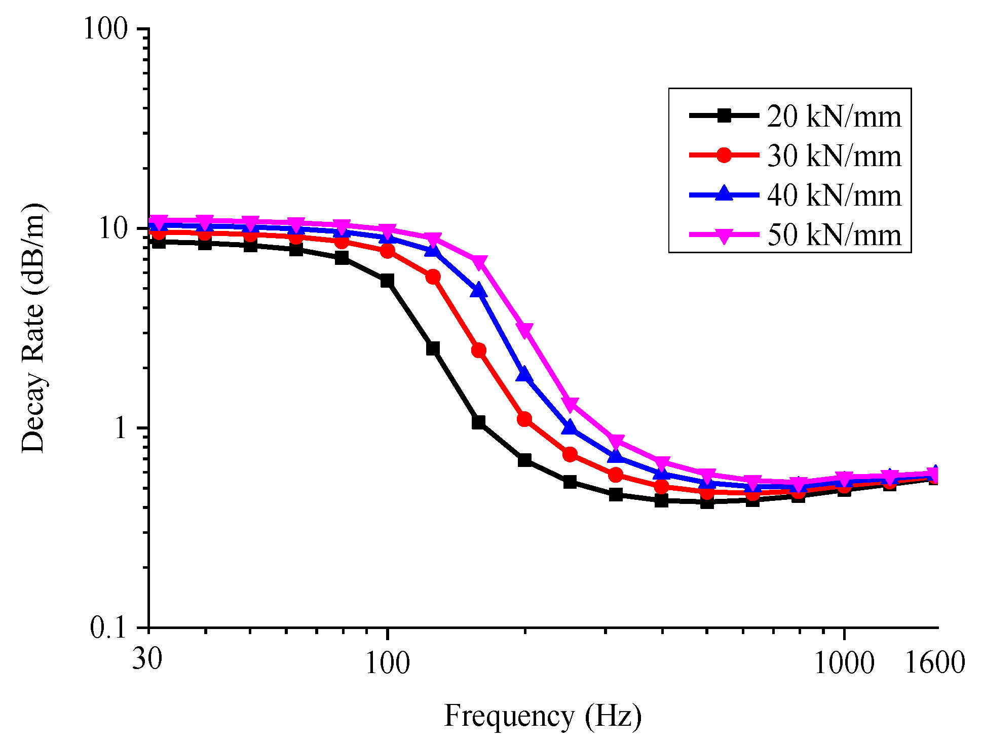
5.2. Influence on the Decay Rate

The simulated influence of the vertical fastener stiffness on the decay rate is shown in Figure 15 (in the form of the one-third octave spectra):

The increase of the vertical fastener stiffness will strengthen the coupling between the rail and the sleeper. Thus, the DR increases below the center frequency of 1600 Hz, and more vertical rail vibration energy is transmitted in the downward direction. Besides, as the boundary frequency of the high DR band, i.e., f_v, is increased, the high DR band also gets widened. When the vertical rail resonance frequency increases from f_v to f_v^*, the most significant increase of the DR is in the frequency range of f_v to f_v^*. However, the influence of vertical fastener stiffness on the DR is not obvious in the high-frequency range.

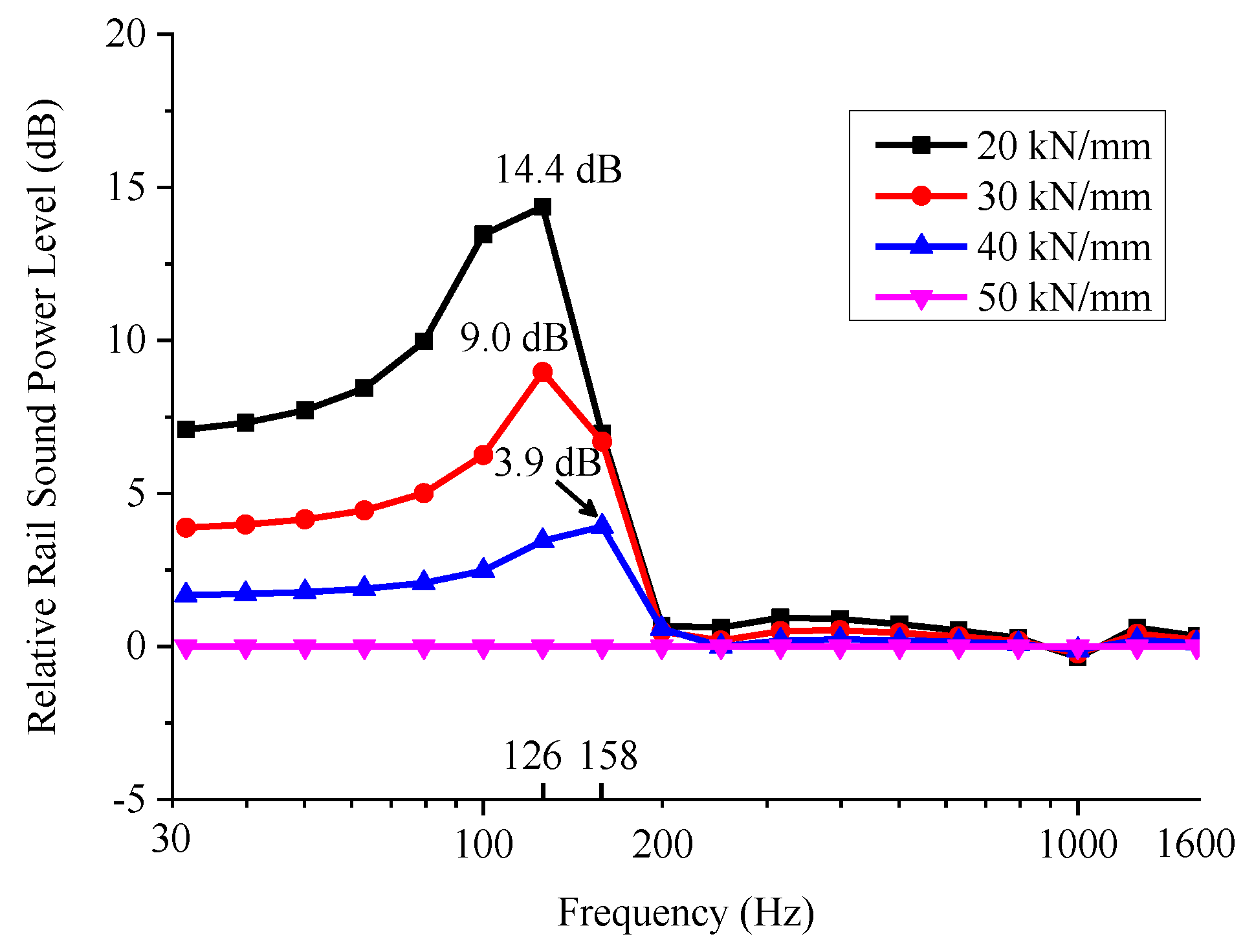
5.3. Influence on the Rail Sound Power Level

In order to directly elaborate the influence of vertical fastener stiffness at different frequencies, the relative sound power level of the rail subjected to a harmonic point excitation is investigated in this section, while the rail sound power level with the vertical fastener stiffness of 50 kN/mm is taken as the reference. The simulated influence of the vertical fastener stiffness on the relative sound power level of the rail subjected to a harmonic point excitation is shown in Figure 16 (in the form of the one-third octave spectra).

When the vertical fastener stiffness decreases from 50 kN/mm, the rail sound power level below the center frequency of 200 Hz gets increased. More rail vibration energy spreads outward in the form of sound energy. For each relative rail sound power level curve, a peak appears at the center frequency close to the decreased vertical rail resonance frequency, where the increase of rail sound power level is most significant. In the corresponding one-third octave band, the rail mobility amplitude increases significantly while the decay rate decreases considerably. At the center frequency of 126 Hz, the rail sound power level with the stiffness of 20 kN/mm is 14 dB higher than that with the stiffness of 50 kN/mm. The influence of vertical fastener stiffness on the rail sound power level is small above the center frequency of 200 Hz.

6. Conclusions

The main conclusions can be drawn as follows:

(1) Below the center frequency of 800 Hz, the sound power level of the rail subjected to the harmonic point excitation increases with the increase of frequency. A peak appears at the center frequency of 800 Hz mainly because the rail radiation ratio peaks near the center frequency of 800 Hz.

(2) With the increase of the vertical fastener stiffness, the vertical rail resonance frequency increases while the value of the corresponding peak in the direct mid-span rail mobility amplitude curve decreases slightly. Meanwhile, the decay rate increases below the center frequency of 1600 Hz. When the vertical rail resonance frequency increases from f_v to f_v^*, the mobility amplitude below f_v decreases while that above f_v^* increases. The maximal decrease and increase occur at f_v and f_v^*, respectively. The most significant increase of the decay rate is in the frequency range of f_v to f_v^*.

(3) When the vertical fastener stiffness decreases from 50 kN/mm, the sound power level of the rail subjected to a harmonic point excitation below the center frequency of 200 Hz gets increased. The increase of the sound power level is most significant at the center frequency close to the decreased vertical rail resonance frequency, because in the corresponding one-third octave band the rail mobility amplitude increases significantly while the decay rate decreases considerably.

We suggest that the adoption of the vibration-mitigation measures should be accompanied with the corresponding noise investigation. The optimal value of the vertical fastener stiffness should be determined by the vibration-noise conjoint analysis and optimization.

References

1. Gupta, S.; Degrande, G.; Lombaert, G. Experimental validation of a numerical model for subway induced vibrations. J. Sound Vib. 2009, 321, 786–812. [Google Scholar] [CrossRef]
2. Thompson, D.J. Railway Noise and Vibration: Mechanisms, Modelling and Means of Control; Elsevier Limited: Oxford, UK, 2008; pp. 195–196. [Google Scholar]
3. Knothe, K.; Wu, Y. Receptance behaviour of railway track and subgrade. Arch. Appl. Mech. 1998, 68, 457–470. [Google Scholar] [CrossRef]
4. Kaewunruen, S.; Remennikov, A.M. Field trials for dynamic characteristics of railway track and its components using impact excitation technique. NDT E Int. 2007, 40, 510–519. [Google Scholar] [CrossRef]
5. Oregui, M.; Li, Z.; Dollevoet, R. An investigation into the vertical dynamics of tracks with monoblock sleepers with a 3D finite-element model. Proc. Inst. Mech. Eng. Part F J. Rail Rapid Transit 2016, 230, 891–908. [Google Scholar] [CrossRef]
6. Arlaud, E.; D’Aguiar, S.C.; Balmes, E. Receptance of railway tracks at low frequency: Numerical and experimental approaches. Transp. Geotech. 2016, 9, 1–16. [Google Scholar] [CrossRef]
7. Jones, C.J.C.; Thompson, D.J.; Diehl, R.J. The use of decay rates to analyse the performance of railway track in rolling noise generation. J. Sound Vib. 2006, 293, 485–495. [Google Scholar] [CrossRef]
8. Squicciarini, G.; Toward, M.G.R.; Thompson, D.J. Experimental procedures for testing the performance of rail dampers. J. Sound Vib. 2015, 359, 21–39. [Google Scholar] [CrossRef] [Green Version]
9. Betgen, B.; Squicciarini, G.; Thompson, D.J. On the prediction of rail cross mobility and track decay rates using Finite Element Models. In Proceedings of the 10th European Congress and Exposition on Noise Control Engineering, Maastricht, The Netherlands, 31 May–3 June 2015. [Google Scholar]
10. Li, W.; Dwight, R.A.; Zhang, T. On the study of vibration of a supported railway rail using the semi-analytical finite element method. J. Sound Vib. 2015, 345, 121–145. [Google Scholar] [CrossRef]
11. Vincent, N.; Bouvet, P.; Thompson, D.J.; Gautier, P.E. Theoretical optimization of track components to reduce rolling noise. J. Sound Vib. 1996, 193, 161–171. [Google Scholar] [CrossRef]
12. Zhang, X.; Squicciarini, G.; Thompson, D.J. Sound radiation of a railway rail in close proximity to the ground. J. Sound Vib. 2016, 362, 111–124. [Google Scholar] [CrossRef] [Green Version]
13. Lee, U.; Kim, D.; Park, I. Dynamic modeling and analysis of the PZT-bonded composite Timoshenko beams: Spectral element method. J. Sound Vib. 2013, 332, 1585–1609. [Google Scholar] [CrossRef]
14. Igawa, H.; Komatsu, K.; Yamaguchi, I.; Kasai, T. Wave Propagation Analysis of Frame Structures Using the Spectral Element Method. J. Sound Vib. 2004, 277, 1071–1081. [Google Scholar] [CrossRef]
15. Lee, U. Spectral Element Method in Structural Dynamics; John Wiley and Sons: New York, NY, USA, 2009; pp. 365–369. [Google Scholar]
16. Sheng, X.; Zhao, C.; Wang, P.; Liu, D. Study on Transmission Characteristics of Vertical Rail Vibrations in Ballast Track. Math. Probl. Eng. 2017, 2017, 5872419. [Google Scholar] [CrossRef] [Green Version]
17. Wei, K.; Wang, P.; Yang, F.; Xiao, J. The effect of the frequency-dependent stiffness of rail pad on the environment vibrations induced by subway train running in tunnel. Proc. Inst. Mech. Eng. Part F J. Rail Rapid Transit 2016, 230, 697–708. [Google Scholar] [CrossRef]
18. Thompson, D.J. Wheel-rail Noise Generation, Part III: Rail Vibration. J. Sound Vib. 1993, 161, 421–446. [Google Scholar] [CrossRef]
19. Bulgakov, E.N.; Sadreev, A.F.; Maksimov, D.N. Light trapping above the light cone in one-dimensional arrays of dielectric spheres. Appl. Sci. 2017, 7, 147. [Google Scholar] [CrossRef] [Green Version]
20. Ryue, J.; Thompson, D.J.; White, P.R.; Thompson, D.R. Decay rates of propagating waves in railway tracks at high frequencies. J. Sound Vib. 2009, 320, 955–976. [Google Scholar] [CrossRef]
21. Thompson, D.J.; Vincent, N. Track Dynamic Behaviour at High Frequencies. Part 1: Theoretical Models and Laboratory Measurements. Veh. Syst. Dyn. 1995, 24, 86–99. [Google Scholar] [CrossRef]
22. Man, A.P.D. A Survey of Dynamic Railway Track Properties and Their Quality. Ph.D. Thesis, Delft University of Technology, Delft, The Netherlands, 2002. [Google Scholar]
23. CEN. EN 15461:2008+A1:2010, Railway Applications—Noise Emission—Characterization of the Dynamic Properties of Track Selections for Pass by Noise Measurements; Management Center: Brussels, Belgium, 2010. [Google Scholar]
24. Thompson, D.J. Experimental analysis of wave propagation in railway tracks. J. Sound Vib. 1997, 203, 867–888. [Google Scholar] [CrossRef]
25. Ewins, D.J. Modal Testing: Theory and Practice; Research studies Press: Letchworth, UK, 1984. [Google Scholar]
Figure 1. The monolithic track bed structure: (a) Photograph and (b) Sectional view.
Applsci 10 01682 g001
Figure 2. The Timoshenko-beam track model.
Applsci 10 01682 g002
Figure 3. The element division using the spectral element method.
Applsci 10 01682 g003
Figure 4. Two-node spectral Timoshenko beam element.
Applsci 10 01682 g004
Figure 5. One-node Timoshenko beam right-throw-off element.
Applsci 10 01682 g005
Figure 6. The periodic track model.
Applsci 10 01682 g006
Figure 7. The element division of the periodic track model.
Applsci 10 01682 g007
Figure 8. The field measurement of the rail accelerance.
Applsci 10 01682 g008
Figure 9. The accelerometer and the hammer impact positions.
Applsci 10 01682 g009
Figure 10. Amplitude of direct vertical rail accelerance.
Applsci 10 01682 g010
Figure 11. Amplitude of direct vertical rail mobility.
Applsci 10 01682 g011
Figure 12. Decay rate.
Applsci 10 01682 g012
Figure 13. Sound power level of the rail subjected to a harmonic point excitation.
Applsci 10 01682 g013
Figure 14. Influence of vertical fastener stiffness on direct mid-span rail mobility amplitude.
Applsci 10 01682 g014
Figure 15. Influence of vertical fastener stiffness on the decay rate (DR).
Applsci 10 01682 g015
Figure 16. Influence of vertical fastener stiffness on the relative rail sound power level.
Applsci 10 01682 g016