Thermal Property Evaluation of Porous Asphalt Concrete Based on Heterogeneous Meso-Structure Finite Element Simulation

Abstract

Porous asphalt concrete (PAC) can obviously improve vehicle driving safety on rainy days and reduce environmental noise. It has been widely used in China. The existence of a large number of interconnected voids in PAC makes a significant difference in heat transfer and temperature distribution from conventional dense-graded asphalt concretes (AC). In this paper, the internal structure images of three dense-graded asphalt mixtures and one PAC were obtained by X-ray CT scanning technology, and the internal meso-structure finite element simulation models of asphalt mixtures were established by using the mapped meshing method. The temperature variations of asphalt mixture specimens during laboratory cooling and heating processes were simulated in this study, and laboratory tests were carried out to verify the simulation accuracy. Due to the simulation results, it was found that the thermal characteristics of the PAC mixture were different from those of the dense-graded asphalt mixture due to the large interconnected air void content in the PAC mixture. The temperature field in the PAC mixture was more sensitive to ambient air temperature under laboratory conditions. Moreover, in PAC specimens, temperature distributed more unevenly than in dense-grade asphalt mixtures. Therefore, it is necessary to consider the internal meso-structure of porous asphalt mixtures while simulating the temperature field in PAC specimens or pavement structures.

1. Introduction

Porous asphalt concrete (PAC) has been widely used because of its good driving safety in rainy days and low noise to the ambient environment. However, the internal void rate of PAC is higher, usually more than 18%, and more than 80% of them are connected with the air outside [1], which intensifies the heat exchange between PAC and the external environment. Therefore, compared to dense-graded asphalt concrete (AC), the thermal characteristics may be very different.

At present, research on the temperature field of asphalt concrete is mainly divided into several directions, such as field measurements of asphalt pavement, laboratory thermal property tests for asphalt mixture specimens and asphalt pavement thermal models and simulations. In field measurements of asphalt pavement, Mallick et al. [2,3] studied the effect of buried pipelines on the pavement temperature field. In a laboratory thermal property test for an asphalt mixture specimen, Hassn [4] irradiated dry saturated asphalt slabs with different voids in the laboratory and measured the surface and bottom temperature evolution, heat flux and evaporation rate, and the effect of voids on the temperature evolution of asphalt mixtures under dry and wet conditions were quantified. Luca [5] discussed a new laboratory method for measuring the thermal properties of asphalt concrete specimens and proved that there was no correlation between the thermal properties and physical properties of asphalt concrete. Nguyen et al. [6] studied the temperature changes of asphalt mixture cylindrical specimens during the cyclic test and determined the thermal conductivity and convective heat transfer coefficient of asphalt mixture in a steady-state. Islam et al. [7] measured thermal conductivity and specific heat capacity of asphalt mixtures in the laboratory and validated them with strain and temperature data collected on the instrument pavement section of Interstate Highway 40 near Albuquerque, New Mexico.

In the study of a temperature field model, Gui et al. [8] established a one-dimensional mathematical model based on the basic energy balance and used hourly data of solar radiation, temperature, dew point temperature and wind speed to calculate the surface temperature of the pavement. Qin [9] studied the effect of air temperature on the temperature distribution of rigid pavement slab thickness, and one kind of one-dimensional heat transfer model was proposed to predict pavement temperature distribution. Xu [10] discussed the analysis model for predicting the transient temperature distribution in asphalt concrete, and the relationship between thermal conductivity and convective heat transfer coefficient was obtained. Chen et al. [11] proposed a new evaluation model of thermal conductivity of asphalt concrete with non-uniform structure and predicted the effective thermal conductivity of asphalt concrete. Wang [12] deduced the basic effective thermal conductivity structure model and calculated the effective thermal conductivity of the heterogeneous composites. Yavuzturk [13] built a transient two-dimensional finite difference model to evaluate temperature fluctuations of asphalt pavement under the thermal environment. In order to calculate the pavement temperature in northeastern Portugal, Minhoto [14] established a three-dimensional finite element (FE) model of a multi-layer pavement structure for transient thermal analysis. The results showed that three-dimensional finite element analysis is an effective tool to simulate the transient characteristics of asphalt concrete pavement. The simulation model can predict the pavement temperature of different pavement layers. Based on the finite element method, a two-dimensional numerical model of asphalt concrete was established by Mirzanamadi et al. [15] to investigate the effects of different design parameters and environmental conditions on the thermal properties (thermal conductivity, diffusivity and specific heat capacity) of asphalt concrete.

In the temperature field analysis of porous asphalt concrete (PAC), a one-dimensional pavement temperature model developed by Arizona State University was used by Stempihar et al. [16] to simulate the surface temperature of porous asphalt, traditional dense-graded asphalt and Portland cement concrete pavement. However, different thermal parameters were adopted rather than the difference between mixture gradations, void rates and meso-structures to reflect thermal conductivity difference between PAC and dense-graded AC mixtures. Hassn [17] studied the thermal conductivity of PAC and dense-graded AC by laboratory tests. It was proved that the lower specific heat capacity and thermal conductivity of PAC were the reasons for the faster cooling and heating rate than AC mixtures.

In all the above studies, a large number of monitoring points needed to be laid out for field measurement and long-term observation. The costs can be very high, the number of monitoring points might be limited, and there are many interference factors; the accuracy of results cannot be ensured. A laboratory test has higher accuracy and various influencing factors can be evaluated, but a large number of specimens needs to be fabricated, and temperature sensors should be repeatedly installed on each specimen. The studies based on laboratory tests are usually cumbersome and time-consuming.

More importantly, during temperature laboratory tests, sensors need to be installed by means of pre-burying and drilling in asphalt mixture specimens, which disturbs and damages the internal structure of asphalt mixtures and is a major disadvantage to the accurate measurement of temperature. Heat conduction analysis based on the three-dimensional finite element model has been proved to be an effective means to study the temperature field of a material or pavement structure and can freely change various influencing factors, so as to evaluate the importance of influencing factors.

However, in present finite element simulations, asphalt concrete was usually regarded as homogeneous material in the calculation of the temperature field, so uniform thermal parameters were set during the calculation process. This method may be feasible for dense-graded asphalt concrete with little air voids. However, for PAC with a large number of interconnected voids and discontinuous gradation, the internal temperature field exists in a non-uniform and discontinuous state, so the internal structure cannot be regarded as a homogeneous form. Therefore, the purpose of this paper is to introduce the asphalt mixture internal meso-structure into the thermal simulation by using a finite element method for evaluation.

2. Objectives

• Introducing the heterogeneous structure of asphalt mixture into laboratory temperature field simulation, establishing finite element simulation model while considering asphalt mixture heterogeneous meso-structure;
• Verifying the validity of the FE model by comparing with laboratory tests;
• Comparing the temperature field variation rules and influencing factors of a gap-gradation PAC mixture and dense-graded AC mixtures.

3. Asphalt Mixture Meso-Structure Modeling Technology

At present, there are two methods for three-dimensional heterogeneous structure modeling of asphalt mixtures; one is image-based (IB) modeling technology [18,19], and another is computer-generalized (CG) modeling technology [20,21].

The images used in IB technology can be acquired from X-ray CT scanning. A series of image slices [22,23] can be obtained by industrial CT scanning of asphalt mixture specimens. Then, image enhancement, denoising, threshold division, material separation and three-dimensional reconstruction can be carried out using digital image processing (DIP) technology [24], and the images can be transformed into a finite element model [25]. Thereby, follow-up mechanical or heat transfer simulations can be carried out.

CG technology generates asphalt mixture numerical specimens randomly according to the parameters of aggregate shape, particle size, gradation, void rate, etc. by adopting commercial software or custom program and then imports them into finite element software to mesh and generate an analysis model [26].

As far as the convenience and freedom of modeling are concerned, CG technology has obvious advantages. Only the supports of computer hardware and software are needed; the model can be generated directly. However, IB technology has obvious advantages in terms of accuracy and reducibility of the model. IB technology can theoretically completely restore the internal structure of an asphalt mixture based on CT scanned images of actual specimens.

Therefore, IB technology based on X-ray CT scanned images was selected to model the heterogeneous structure of asphalt mixtures in this paper, so as to restore the internal structure of asphalt mixtures to the greatest extent, which is conducive to improving the accuracy of simulation results.

At present, there are two main methods to generate finite element meshes from an IB generated model: mapped meshing [25,26,27] and free meshing [28,29,30,31]. Among these two methods, the model element established by the mapped meshing method is of a regular shape, the calculation process is more convergent and the analysis results are more reliable. Thus, the mapped meshing method was adopted in this paper, and the detailed modeling process is shown in Figure 1.

The finite element model building process is mainly divided into three steps: specimen preparation, meso-structure modeling and simulation and verification. There are many sub-steps in each step. The process of model building is described in detail in the following sections.

4. Mixture Design and Specimen Preparations

Porous asphalt concrete (PAC) is widely used as the material of the asphalt pavement top layer in high-grade expressways. In China’s expressways, asphalt pavement usually adopts a three-layer structure, and the most commonly used materials are AC-13, AC-20 and AC-25. AC stands for asphalt concrete, and the number represents the maximum nominal particle size of aggregate in the mixtures. When PAC is applied in the pavement, PAC-13 replaces AC-13 as the top layer material. Therefore, four types of asphalt mixtures, namely PAC-13, AC-13, AC-20 and AC-25, were chosen as research objects. The gradations, optimum asphalt contents and void rates of the four asphalt mixtures are shown in

Table 1. Gradation of four types of asphalt mixtures.

Sieve Size (mm)	AC-13	AC-20	AC-25	PAC-13
31.5	100	100	100	100
26.5	100	100	100	100
19	100	96.8	84.5	100
16	100	88.7	74.9	100
13.2	96.2	78.8	67.9	95.7
9.5	76.1	64.8	59.5	64.8
4.75	52.7	40.5	42.7	21.4
2.36	37.2	27.3	31.5	13.5
1.18	25.1	18.1	22.6	10.9
0.6	18.1	12	15.8	8.9
0.3	13.3	8.4	10.6	7.3
0.15	10.6	6.6	7.4	6.2
0.075	6.7	5.4	5.4	4.5
Optimal binder content (%)	4.9	4.5	4.2	4.8
Aggregate	Basalt	Basalt	Basalt	Basalt
Void content (%)	4	4	4	20.4

. Because only the thermal properties were of concern in this paper, and the mechanical properties were not involved, all the AC mixture used PG76-22 asphalt as the binder, while PAC-13 used high-viscosity asphalt (HVA) as the binder. HVA is typically used in China to improve the raveling resistance and strength of PAC [32]. HVA is characterized by extremely high kinetic viscosity and softening point. The kinetic viscosity at 60 °C of HVA used in this study was 143,202 Pa∙s and the softening point was 91 °C.

Four specimens of each mixture type were fabricated by a Superpave gyratory compactor (SGC) with 50 gyrations, with 100 mm in diameter and 63.5 mm in height.

5. X-Ray CT Scanning and Finite Element Model Construction

After the specimen fabrications, specimens with better quality were selected for CT scanning to obtain the images of mixture internal structures. Due to the high cost of industrial CT scanning, in this paper, only one specimen for each type of mixture was selected. After scanning, a series of 8-bit grayscale images at different specimen depths were obtained. The depth interval between adjacent image slices was 0.06 mm, and about 1100 image slices were obtained during the CT scanning process for each specimen. Otsu’s algorithm was used to confirm the optimum thresholds during the image segmentation procedure, and then air voids, asphalt mortar and aggregates were segmented by different gray values. Finally, each original grayscale CT slice image was transformed into three binary images to present the air voids, asphalt mastic and coarse aggregate, respectively, as shown in Figure 2b–d.

Based on the processed images, the modeling method and mapped meshing technology showed in Figure 1 were utilized to generate finite element models of four kinds of asphalt mixtures using the MATLAB program. The meso-structure models of four kinds of asphalt mixtures are shown in Figure 3. The gray part represents aggregate and the dark blue area represents asphalt mortar.

6. Region Segmentation of the Finite Element Model

In order to investigate the temperature field difference at different locations in specimens, each specimen was divided into four regions along the radial direction, numbered A, B, C and D, and five regions along the height direction, numbered 1–5, as shown in Figure 4.

Therefore, each specimen was divided into 20 regions. For example, region D1 represented the region of the top and outermost circle of the specimen. Region A3 represented the most central region of the specimen. In addition, each region could be divided into three different materials (asphalt mortar, aggregate, void) represented by AS, AG and VO, respectively. For example, D1_AS represented mortar in region D1, and A3_AG represented aggregate in region A3.

7. Heat Transfer Theory in Asphalt Mixture Meso-Structure

This study focused on the thermal properties of an asphalt mixture under laboratory conditions; the variation laws and influencing factors of temperature fields had to be investigated, so transient heat transfer analysis was adopted. Combining the first law of thermodynamics (i.e., the conservation of heat energy) and Fourier’s law (i.e., the relationship between heat flux and thermal gradient), the following formulas can be used for calculating asphalt mixture heat transfer characteristics [14].

$${\nabla }^{2}T=\frac{1}{\alpha }\times \left(\frac{\partial T}{\partial t}\right)$$

(1)

$${\nabla }^2=\left({\partial }^2/\partial x^2\right)+\left({\partial }^2/\partial y^2\right)+\left({\partial }^2/\partial z^2\right)$$

(2)

• $\alpha =\frac{k}{\rho \times C}$ = thermal diffusivity,
• k = thermal conductivity,
• $\rho$ = density,
• C = specific heat,
• T = temperature,
• t = time, and
• x,y and z = components of the Cartesian coordinate system

The meso-structure of the asphalt mixture was no longer continuous, due to the consideration of the heterogeneous structure in this paper, but for each material component, such as asphalt mortar and aggregate, they could be regarded as homogeneous materials separately. Therefore, the above three-dimensional heat transfer theory was still applicable in the analysis of the temperature field of asphalt mixture heterogeneous meso-structures.

8. Heat Interaction between Laboratory Specimens and Surrounding Air

The surfaces of asphalt mixture specimens were exposed to the air environment, and the heat transfer by energy interaction between specimen and its surroundings consists of thermal radiation flux and convection heat flux. The total heat flux can be expressed as follows [13].

$$q_{surf}=q_r+q_c$$

(3)

where $q_r$ is surface thermal radiation flux, and $q_c$ is convection heat transfer.

8.1. Specimen Surface Thermal Radiation Flux

The surface thermal radiation flux can be considered through the following expression:

$$q_r=h_r\left(T_{surf}-T_{air}\right)$$

(4)

where $q_r$ is thermal radiation flux on specimen surface, and $h_r$ is the thermal radiation coefficient. The expression used to obtain $h_r$ is as follows:

$$h_r=\epsilon \sigma \left(T_{surf}+T_{air}\right)\left(T_{surf}^2+T_{air}^2\right)$$

(5)

where $\epsilon$ is the emissivity of the pavement surface, $\sigma$ is Stefan–Boltzmann constant, $T_{surf}$ is specimen surface temperature and $T_{air}$ is ambient air temperature.

8.2. Pavement Surface Convection Heat Flux

The convection heat flux generated between the specimen surface and ambient air can be expressed as follows:

$$q_c=h_c\left(T_{surf}-T_{air}\right)$$

(6)

where $h_c$ is the convection heat transfer coefficient.

9. Thermal Properties of Asphalt Mixture Components

The meso-structure of asphalt mixtures was considered in this study. The asphalt mixture was regarded as a three-phase structure composed of asphalt mortar (asphalt and aggregate with particle size less than 2.36 mm), coarse aggregate and void. Therefore, according to the above heat conduction theory, it was necessary to determine the thermal parameters of each component of the asphalt mixture.

Based on the investigation of the existing research [33], the thermal parameters of asphalt mixture components suitable for the above heat transfer theory were determined, as shown in

Table 2. Thermal properties of asphalt mixture components.

Thermal Property	Symbols and Units	Asphalt Mortar	Aggregate	Air Void
Conductivity	$k\left(\mathrm{J}/\left(\mathrm{mm}\cdot \mathrm{h}\cdot ℃\right)\right)$	vary with temperature	vary with temperature	0.0828
Density	$\rho \left({\mathrm{kg}/\mathrm{mm}}^3\right)$	1.05 × 10−6	2.8 × 10−6	1.225 × 10−9
Specific heat capacity	$C\left(\mathrm{J}/\left(\mathrm{kg}\cdot ℃\right)\right)$	vary with temperature	vary with temperature	1.005
Pavement surface emissivity	$\epsilon$	0.81	0.81	-
Convection heat transfer coefficient	$h_c\left(\mathrm{J}/\left({\mathrm{mm}}^2\cdot \mathrm{h}\cdot ℃\right)\right)$	2.4466 × 10−2	9.2048 × 10−2	-
Absolute temperature zero	$T_Z(℃)$	−273
Stefan–Boltzmann constant	$\sigma \left(\mathrm{J}/\left(h\cdot {\mathrm{mm}}^2\cdot {℃}^4\right)\right)$	2.041092 × 10−10

. It should be noteworthy that most of the parameters have little correlation with temperature and can be considered as constant values. However, thermal conductivity and specific heat capacity are two parameters that vary with temperature, which need to determine the law of change with temperature.

In addition, the geometric dimension unit of the asphalt mixture finite element model established in this paper is millimeter (mm), and the time unit during the analysis process is the hour (h). Therefore, the units of the corresponding thermal parameters must be converted.

9.1. Specific Heat Capacities of Asphalt Mortars and Aggregates

As shown in Table 2, the specific heat capacity and thermal conductivity of aggregate and asphalt mortar vary with temperature. Considering specific heat capacity first, the specific heat capacities of asphalt, aggregate and mineral powder were measured by Lihong et al. [34], as

Table 3. Specific heat capacities of asphalt mixture components at different temperatures.

Temperature (°C)	$\mathbf{Specific}\mathbf{Heat}\left(\mathbf{J}/\mathbf{kg}\cdot ℃\right)$
	Asphalt	Aggregate	Mineral Filler
0	1583	808	803
10	1633	820	822
20	1706	831	844
25	1725	837	852
30	1707	843	861
35	1723	850	871
40	1758	855	879
45	1829	862	890
50	1865	868	899
55	1863	873	910
60	1870	880	920
65	1904	886	930
70	1938	891	939
75	1976	896	950
80	1967	902	960

shows. It can be found that the specific heat capacities of aggregate and mineral powder in asphalt mixture have a strict linear correlation with temperature, and the relationship between asphalt and temperature has a quasi-linear correlation. The specific heat capacity of aggregate was used directly in this study, but asphalt mortar contains asphalt, fine aggregate and mineral powder. At present, there is no related research to directly measure the specific heat capacity of asphalt mortar.

According to the existing research achievements [35], the specific heat capacity of multiphase composites can be calculated according to the following formula:

$$C=\frac{{\displaystyle \sum _{i=1}^n{m}_i{C}_i}}{M}={\displaystyle \sum _{i=1}^n{p}_i{C}_i}$$

(7)

where C is the specific heat capacity of composite, M is the mass of composites, $m_i$ is the mass of each component, $C_i$ is the thermal conductivity of each component, n is the number of components and $p_i$ is the mass percentage of each component.

According to the aggregate gradations and asphalt contents of the asphalt mixtures shown in Table 1, the mass contents of each component in asphalt mortars can be calculated, as shown in Figure 5.

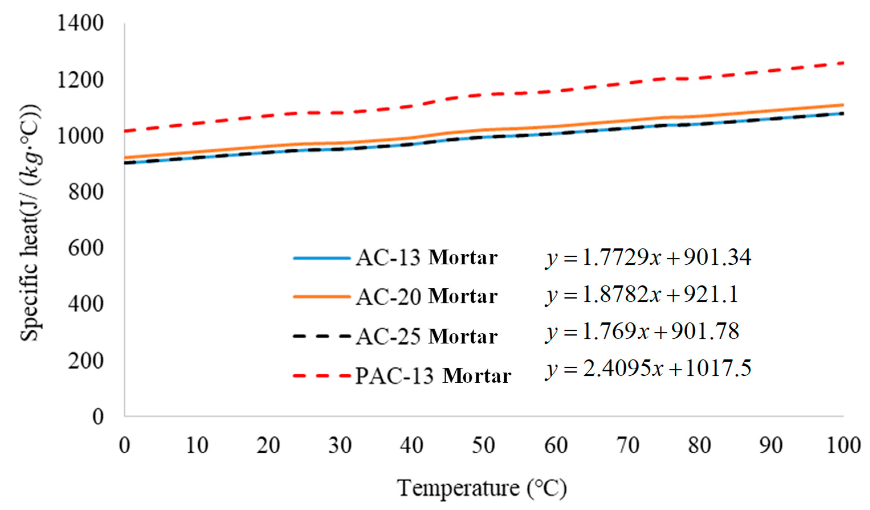
According to the mass contents of each component shown in Figure 5 and the specific heat capacity at different temperatures of each component in Table 3, the asphalt mortar specific heat capacity variation law with temperature can be obtained, as shown in Figure 6.

As shown in Figure 6, it can be found that the specific heat capacities of asphalt mortars in four different asphalt mixtures are quasi-linearly related to temperature. Therefore, the four quasi-linear lines shown in Figure 6 were fitted in this paper, and the fitting equations were also listed. Among them, the specific heat capacities of AC-13 and AC-25 mortars were almost the same, which was mainly due to the close mass contents of internal components. The specific heat capacity of PAC-13 mortar was the largest, mainly caused by the relatively high mass content of asphalt, which has a larger specific heat capacity. In this paper, the fitting equations shown in Figure 6 were input into ABAQUS software, which automatically calculated the specific heat capacities according to material temperature.

9.2. Thermal Conductivities of Asphalt Mortar and Aggregate

As for the thermal conductivity of asphalt mortar and aggregate, existing research conclusions [36] show that when the temperature changes, the thermal conductivity of any material will change, and the formula between thermal conductivity and temperature is satisfied as to the followed formula.

$$\lambda ={\lambda }_0\left(1+bT\right)$$

(8)

where b is the temperature coefficient, which is usually constant; ${\lambda }_0$ is the thermal conductivity of material at 0 °C; and T is temperature. In a wide temperature range, this linear formula can be used for calculating thermal conductivities of asphalt and aggregate.

According to existing research [37,38], ${\lambda }_0$ and $b$ of basalt aggregate and asphalt are shown in

Table 4. Thermal conductivities of asphalt mixture components.

Mixture Components	Parameters
	${\mathit{\lambda }}_0$$(\mathbf{W}/\left(\mathbf{m}·℃\right))$	$\mathit{b}$
Basalt aggregate	2.4757	5.22 × 10−3
Asphalt	0.1227	1.2 × 10−2

.

Similar to the specific heat capacity calculation process, the thermal conductivity of asphalt mortar also needs to be calculated. Williamson [39] studied the thermal conductivity of the asphalt mixture in 1972 and put forward the calculation formula as follows:

$$k_m={\left(k_a\right)}^m\cdot {\left(k_b\right)}^n\cdot {\left(k_v\right)}^p\cdot {\left(k_w\right)}^q$$

(9)

where $k_m$, $k_a$, $k_b$, $k_v$, $k_w$ are the thermal conductivities of the mixture, aggregate, asphalt, air and water, respectively, and m, n, p, q represent the volume contents of aggregate, asphalt, air and water, respectively.

It can be considered that there is almost no air and water in asphalt mortar, so only the effects of asphalt and aggregate should be considered in the formula above. Combining the density of each component, the volume contents of each component in mortars can also be calculated according to the mixture gradations shown in Table 1. All volume contents are expressed in percentages, as shown in Figure 7.

The thermal conductivities of asphalt mortars can be calculated according to the volume contents of each component in Figure 7 and the thermal conductivities of each component in Table 4, as Figure 8 shows:

According to the results shown in Figure 8, the thermal conductivities of asphalt mortar are linearly related to temperature. Because the volume contents of components are very close, the thermal conductivities of AC-13 and AC-25 were almost the same. Due to the thermal conductivity of asphalt being much smaller than that of aggregate, the thermal conductivity of PAC-13 mortar with higher asphalt content was lower. The straight lines shown in Figure 8 were fit by linear equations and input into ABAQUS software for simulations.

10. Verification of Thermal Simulation Model Validity by Laboratory Test

In order to verify the validity of simulation models, laboratory tests were carried out to observe the temperature variation of asphalt mixture specimens during the cooling and heating process. During the cooling process, asphalt mixture specimens of four different aggregate gradations (AC-13, AC-20, AC-25 and PAC-13) were put into the 100 °C oven for more than four hours; then the specimens were taken out and quickly transferred into thermal insulation cabinet with 20 °C.

Through the automatic infrared temperature sensor set in the thermal insulation cabinet, the surface temperature data of the specimens were collected, and the temperature variation curves of specimens were drawn. The data collection processes were all set to be 90 min. Because it is a non-destructive test, the same batch of specimens was tested twice in this study to reduce the error and random variability.

During the laboratory heating process, the initial temperatures of specimens were set to 20 °C by the same method mentioned above, and the temperature variations of specimens were recorded under 100 °C ambient temperature.

In the simulation processes, the same conditions as laboratory tests were set. The temperature fields of these four kinds of mixtures were calculated by meso-structure thermal simulation models in ABAQUS software. The specimen temperature data was extracted, and the temperature curves during cooling and heating processes were drawn, respectively, as shown in Figure 9. Exp1_1 represents the first experimental test data during the cooling process, Exp2_2 represents the second experimental test data during the heating process, Sim1 and Sim2 represent the simulation data during the cooling and heating process, respectively, and so on.

It can be found that the simulation results of various asphalt mixtures are in good agreement with the laboratory test results. In order to evaluate the consistency between the results of simulations and laboratory tests, the Pearson correlation coefficient (PCC) was introduced in this paper. The calculation formula of PCC is as follows:

$$\rho \left(X,Y\right)=\frac{\mathrm{cov}\left(X,Y\right)}{{\sigma }_X{\sigma }_Y}=\frac{{\displaystyle \sum _{i=1}^n\left(X_i-\overline{X}\right)\left(Y_i-\overline{Y}\right)}}{\sqrt{{\displaystyle \sum _{i=1}^n{\left(X_i-\overline{X}\right)}^2}}\sqrt{{\displaystyle \sum _{i=1}^n{\left(Y_i-\overline{Y}\right)}^2}}}$$

(10)

in this formula, $X$ and $Y$ are two columns of n-dimensional vectors. Because the specimen data recording frequencies in laboratory tests were not consistent with the simulation analysis, the results of the experiment and simulation were interpolated by MATLAB software first, and then the PCC values between them were calculated directly by corrcoef command in MATLAB.

The average PCC values between the experimental and simulation results during cooling and heating processes are shown in Figure 7 as $\rho \left(\mathrm{Exp},\mathrm{Sim}\right)$. It can be seen from the figures that the PCC values of all mixtures were above 0.997, showing high degrees of consistency. Therefore, the simulation model and analysis parameters adopted in this paper were proved to be effective and reliable in temperature field analysis.

11. The Concept of Temperature Accumulation

According to Figure 7, under the same external conditions, the temperature change curves of various asphalt mixtures are very similar; the temperature change of four asphalt mixtures represents a uniform law, with only some differences in aspect of temperature change rate. The difference in temperature change rate reflects the difference in the thermal stability of asphalt mixtures, and it can be reflected by the material thermal storage coefficient in traditional research.

While a single material layer with enough thickness is affected by harmonic thermal action on the surface, the surface wave amplitude ratio of heat flux and temperature is defined as a thermal storage coefficient. It can be seen from the definition that it is very difficult to obtain the thermal storage coefficient of asphalt mixture accurately, whether during laboratory tests or numerical simulations. Therefore, the concept of temperature accumulation (TA) was introduced to describe the thermal stability differences of various materials under the same environmental conditions.

Temperature accumulation is widely used in biology. It usually refers to the cumulative value of the effective temperature required by plants and oviparous animals to complete a certain development stage, such as the egg hatching process of poultry animals. Similar phenomena also exist in the pavement, such as the obvious acceleration of rutting development when the pavement temperature is higher than a certain limit value. In this paper, TA is introduced mainly to describe the thermal stability of the material, so TA is expressed as the product value of temperature absolute value and time.

As Figure 10 shows, temperature accumulation is actually the area between the temperature-time curve and the coordinate axes. For two materials with the same initial temperature and environmental temperature, faster cooling means a smaller TA. As shown in the figure, TA2 is significantly smaller than TA1. In contrast, during the heating process, the larger TA means temperature increasing more rapidly. Therefore, with the help of the concept of TA, when describing the changing law of the temperature field of different materials under the same temperature boundary condition, many similar curves can be omitted, and the thermal stabilities of materials can be directly reflected by temperature accumulation.

12. Influencing Factors of Laboratory Specimen Temperature Variation

In order to study the factors affecting the temperature field distribution inside the mixture, the influencing factors, such as mixture gradation, mixture component and specimen region were considered, and the influences of various factors mentioned above on TA were investigated. Table 1 shows the four mixture types with different aggregate gradations. Mixture components were aggregate, mortar and void, respectively. Specimen regions were defined, as shown in Figure 4. The TA values of different mixtures, different components and different regions during the cooling process (specimen initial temperature was 100 °C, ambient temperature was 20 °C) and heating process (specimen initial temperature was 20 °C, ambient temperature was 100 °C) within 1.5 h was investigated; the results are shown in Figure 11 and Figure 12. The average value (AVG) of TA is shown in each classification block.

12.1. Influence of Asphalt Mixture Gradation

Firstly, the influence of the mixture gradation was investigated. TA values of different mixtures are represented by different icons in the figures. The TA values of AC-20 and AC-25 were very close in both cooling and heating processes, mainly because the thermal characteristics of these two mixtures are more similar, caused by more similar aggregate gradations. In cooling processes, TA values of these two mixtures were larger than that of AC-13, while smaller than that of AC-13 in heating processes, which shows better thermal stability of AC-20 and AC-25 mixtures.

Due to the larger aggregate sizes of AC-20 and AC-25 mixtures, the void sizes in these two mixtures were also larger than AC-13, as the air voids inside the mixtures play a certain role in thermal insulation. Although the void content of the AC-13 mixture was close to that of two other dense-graded asphalt mixtures, the thermal insulation effect of smaller voids in the AC-13 mixture was not as good as that of larger voids in AC-20 and AC-25 mixtures. In addition, the aggregate contents in AC-20 and AC-25 mixtures were higher. According to the specific heat capacities and densities, as shown in Table 2 and Table 3, when aggregate and asphalt mortar have the same mass and absorb or emit the same heat, the temperature change of aggregate is smaller than asphalt mortar. Due to the above two reasons, AC-20 and AC-25 mixtures had better thermal stabilities than the AC-13 mixture.

AC-13 and PAC-13 mixtures had the same maximum nominal sizes of aggregate; by comparing these two mixtures, it can be found that TA values of AC-13 were higher than those of PAC-13 in the cooling process, reflecting better thermal stability. However, during the heating process, TA values of AC-13 were still larger than PAC-13 in most cases, which shows that PAC-13 had better thermal stability.

The main reason for this phenomenon is a large number of connected voids existing in the PAC-13 mixture [1]. In the cooling process, due to the high internal temperature of the specimen, the air molecules in the voids are more active, which is easier to volatilize to the external environment, and heat exchange occurs, leading to a faster temperature drop of the PAC-13 mixture. In the heating process, the temperature of the air in the PAC-13 mixture internal voids is relatively lower than that of the external air, and the activities of internal air molecules are insufficient. In addition, as there is almost no external air flowing during the laboratory tests and numerical simulations, the air in voids of the PAC-13 mixture plays a role in thermal insulation. However, if there is air flowing on specimen surfaces, the cold air can be quickly replaced by external hot air, and the temperature rising rate of PAC should be greater than that of AC mixtures, which was proved in porous asphalt pavement temperature analysis [16]. In summary, the existence of a large number of internal voids is an important factor affecting the thermal property of the PAC mixture, making it different from that of dense-graded asphalt mixtures.

12.2. Influence of Asphalt Mixture Component

The effects of mixture components were also evaluated in this paper; three components, namely aggregate, asphalt mortar and voids, were considered. It should be noted that the voids presented in Figure 11 and Figure 12 were all disconnected voids. As shown in the figures, there were no significant TA value differences between aggregates, mortars and voids, because the aggregates in the mixtures were closely wrapped by asphalt mortar; although there were some differences in the thermal characteristics between asphalt mortar and aggregates, the rapid and sufficient heat conduction made the temperature difference between these two components become very small, and the temperature could be regarded as synchronous variating macroscopically.

A similar rule also existed in the void temperature field. Because the disconnected voids were surrounded by aggregates or mortar, and the volume of every single void was very small, the air temperature in voids was directly affected by the surrounding mortar or aggregates, so the temperature change was almost synchronous. Therefore, it is scientific and reasonable to regard asphalt mixture as homogeneous material in traditional thermal analysis, but it is only applicable to dense-graded asphalt concrete. There are a lot of connected voids in the PAC mixture, so the influence of voids must be fully considered.

12.3. Influence of Specimen Region

The differences between different radial regions (Region_r) of cylindrical specimens were investigated, as shown in Figure 11 and Figure 12. There were four regions along the specimen radial direction, marked as A, B, C and D (see Figure 4 for detailed partition). By observing the TA average (AVG) values in all blocks in Figure 11 and Figure 12, it was found that closer to the central regions of specimens, the TA average values became higher during the cooling process, while in the heating process, outer regions had higher TA average values. This phenomenon is in line with the existing research findings and the general understandings because since the heat transfer occurs between specimen surface and external environment, the temperature of the outer regions’ near-surface should change more rapidly than that of the center region.

The same conclusions can be made according to the temperature variation differences between regions along specimen cylindrical direction, with temperature changes more dramatically in the regions closer to the axial ends of specimens than in the central regions.

From the studies above, it can be found that for every asphalt mixture with different gradations, the temperature variation rates were different in different regions of the specimen; thus, in order to evaluate the difference, 60 TA values of each mixture gradation, as shown in Figure 11 and Figure 12, were used to calculate coefficients of variation (CV) to measure the consistencies of temperature variations. The results are shown in Figure 13.

As Figure 13 shows, both during cooling and heating processes, the coefficients of TA variations (TA_CV) of AC-13 mixture were the smallest, while those of AC-20 were close to AC-25, and those of PAC-13 were the largest. This means that the temperature field distributed more complex and more unevenly in PAC-13 specimens under the same cooling or heating processes, which was caused mainly by the large content of internally connected voids. This conclusion further proves that the PAC mixture cannot be treated as homogeneous material in thermal analysis.

12.4. Importance Analysis for Influencing Factors

The effects of mixture gradations, mixture components, radial and axial regions on the temperature field of asphalt mixture laboratory specimens were discussed above. However, the importance of each influencing factor on temperature field variations is not the same. Therefore, a random forest algorithm proposed by Breiman [40] was introduced to evaluate the importance of various influencing factors on TA value.

Firstly, the Bootstrap resampling method was used to randomly extract multiple autogenous data sets from the original data sets (such as shown in Figure 11 and Figure 12) and generate N training samples to construct N classifier trees (called base classifiers). In each process of building the base classifier, data other than training samples were used as test data, which was called out of bag data sets (OOB). Through the error rate based variable importance measures (VIM_ER) on OOB, the importance of variables was scored and ranked.

The basic principle of VIM_ER is to calculate the difference of OOB error rates before and after randomly substituting each variable so as to measure the importance of the variables. Specifically, in order to obtain the importance score of variables, a random forest from training samples was constructed first, and the error rates of all OOB samples were estimated. Then, one variable in all OOB samples was randomly replaced, and the change of prediction error of OOB samples was calculated before and after the replacement of the independent variable. The greater the change of error, the higher the importance of the independent variable. VIM_ER can be expressed as follows.

$$VI{M}_i^{ER}=\frac{1}{Ntree}{\displaystyle {\sum }_{t=1}^{Ntree}\left(E{R}_{it}-E{R}_{it}^{\prime }\right)}$$

(11)

where $Ntree$ is the number of decision trees in random forests, $E{R}_{it}$ is the error rate corresponding to the No.t tree before variable replacement and $E{R}_{it}^{\prime }$ is the error rate corresponding to the No. t tree after variable replacement.

According to the VIM_ER formula, if $X_i$ is not related to the result, the error rate of OOB samples corresponding to the random replacement of $X_i$ will not change, and $VI{M}_i^{ER}=0$ in theory; on the contrary, if $VI{M}_i^{ER}>0$, the variable $X_i$ is related to the result.

Contribution degree (CD) is used to measure the importance of influencing factors to the results, calculated according to the following formula:

$$C{D}_i=\frac{VI{M}_i^{ER}}{{\displaystyle \sum _{i=1}^{n}VI{M}_i^{ER}}}$$

(12)

where $C{D}_i$ is the contribution degree of no. i influencing factor to the results,$0\le C{D}_i\le 1$, and ${\displaystyle \sum _{i=1}^{n}C{D}_i=1}$.

In this paper, the random forest method was used to evaluate the importance of influencing factors on the asphalt mixture laboratory specimen temperature field, and the contribution degrees of influencing factors were calculated, as shown in

Table 5. Contribution degrees of influencing factors.

Influencing Factor	CD to TA
	Cooling Process	Heating Process
Mixture gradation (AC-13, AC-20, AC-25 and PAC-13)	53.59%	76.83%
Region r (A, B, C, D)	38.87%	21.04%
Region h (1,2,3,4,5)	6.56%	1.53%
Component (aggregate, asphalt mortar, void)	0.98%	0.60%

.

Table 5 shows that among these four factors, asphalt mixture gradation was the main factor affecting the temperature field of laboratory specimens, and its contribution degrees during cooling and heating processes were 53.59% and 76.83, respectively.

Secondly, the radial region (Region r) of cylindrical specimens had a significant effect on the specimen temperature field. The effect of the axial region (Region h) was relatively small, especially during the healing process; the contribution degree was only 1.53%.

Finally, the contribution degrees of mixture components during cooling and heating processes were all less than 1%, indicating that the temperature changes of aggregate, mortar and disconnected voids were highly consistent and synchronous. Therefore, for the dense-graded asphalt mixture, void content was small, and voids were almost disconnected. In the process of thermal analysis, the difference of meso-structure can be neglected, and the mixture can be assumed to be macro-thermal homogeneous material for analysis. However, for the gap-gradation PAC mixture with a large number of connected voids, the influence of connected voids on the heat transfer and temperature field of the mixture should be considered.

13. Conclusions

In this paper, the internal meso-structure images of AC-13, AC-20, AC-25 and PAC-13 asphalt mixtures were obtained by X-ray CT scanning technology, and the finite element simulation models considering heterogeneous meso-structure of mixtures were established by using digital image processing technology and mapped meshing method. According to the thermal properties of aggregate and asphalt, combined with the composition of asphalt mortar, the thermal parameters of asphalt mortar were calculated, and the temperature field variations and influencing factors of laboratory cylinder specimens during cooling and heating processes were investigated. The following conclusions can be obtained:

• There is little difference between temperatures of mortar, aggregate and disconnected voids in asphalt mixtures during both laboratory cooling and heating processes. Therefore, for dense-graded asphalt mixtures with mostly disconnected voids, the mixtures can be regarded as homogeneous materials with uniform thermal properties during thermal simulations, without distinguishing the specific components. However, for PAC mixtures with large contents of internally connected voids, the influence of the mixture meso-structure should be considered during thermal analysis.
• In the processes of temperature variation, temperatures in different regions of a specimen are closer in AC mixtures than PAC mixture, whether near the center or near the edge of the specimen, because there is less void content in dense-graded asphalt mixture, and the heat transfer through the solid is fast and uniform; for PAC mixtures with gap-gradation, there are a lot of connected voids in the interior, which make heat resistances between the solids and results in uneven heat transfer inside the specimen. Therefore, in the same ambient environment, the temperature difference between the surface and center of the PAC specimen is relatively larger than that of the AC specimen, and the temperature and temperature accumulation value of each point in the interior is relatively more discrete.
• By importance analysis of influencing factors, it can be found that the effect of mixture gradation is much greater than the mixture component and specimen regions. This is also mainly caused by the differences of void contents and void distributions between gapped-gradation and dense-graded mixtures.

In summary, the large content of internally connected voids in porous asphalt concrete leads the great thermal property, which is different from dense-graded asphalt concrete. Thus, in thermal analysis, the heterogeneous meso-structure of porous asphalt concrete cannot be ignored; in contrast, it should be fully considered. Furthermore, when it comes to investigation of the rutting potential or aging levels of certain pavement structures with PAC, it is necessary to take the special thermal properties of the porous materials into account.