Abstract
In this paper, with the aim of meeting the requirements of car following, safety, comfort, and economy for adaptive cruise control (ACC) system, an ACC algorithm based on model predictive control (MPC) using constraints softening is proposed. A higher-order kinematics model is established based on the mutual longitudinal kinematics between the host vehicle and the preceding vehicle that considers the changing characteristics of the inter-distance, relative velocity, acceleration, and jerk of the host vehicle. Performance indexes are adopted to represent the multi-objective demands and constraints of the ACC system. To avoid the solution becoming unfeasible because of the overlarge feedback correction, the constraint softening method was introduced to improve robustness. Finally, the proposed ACC method is verified in typical car-following scenarios. Through comparisons and case studies, the proposed method can improve the robustness and control precision of the ACC system, while satisfying the demands of safety, comfort, and economy.
1. Introduction
Traffic safety is facing severe challenges with the continuous growth of highway traffic mileage and car ownership. In the face of severe traffic accidents and environmental issues, intelligent transportation systems (ITSs) and advanced driver assistance systems (ADASs) have been proposed worldwide. ADASs are systems aimed at enhancing active safety and providing a better driving experience for drivers; however, they have recently aroused concerns from a wide range of sources [1]. Adaptive cruise control (ACC) is a newly developed ADAS system and has been an important milestone in the history of driving assistance [2,3]. Aside from the basic functions of a cruise control system, the ACC system has the additional ability to avoid forward collisions and keep a safe distance from the preceding vehicle by considering the relative distance, the relative velocity, and the relative acceleration of the vehicle. Xiao and Gao [4] indicated that the success of ACC can be considered a good example for the development of a complete cooperation ADAS system.
Commonly, ACC systems can reduce the working intensity of the driver and ensure the safety of driving through the automatic control of longitudinal movement, and can provide auxiliary support for drivers through a convenient human–computer interface. At present, most scholars consider car following and safety in the design of ACC strategies. However, comfort and economy are also important performance features for ACC systems. Therefore, the control goal of ACC is to improve the ride comfort and economy on the premise of tracking the expected safe car spacing, with the difficulty being in the construction of multi-objective control strategies involving such features as safety, economy, and comfort. The motivation of this paper is to design an ACC system that can consider the abovementioned multi-objectives, which include safety, comfort, economy, and car following.
For the above multi-objective optimization problem, linear quadratic (LQ) and model predictive control (MPC) are commonly used solutions. For automotive applications, nonlinearity and constraint problems must be considered. The realization of LQ needs an implicit assumption with no external disturbance. However, the ACC system has external disturbances, with the state of the preceding vehicle causing a standard LQ regulator to lose its optimality to a certain extent. It is important to consider that MPC is capable of optimally controlling constrained nonlinear problems in each step by rolling optimization while LQ cannot. Since the above optimization problem is non-nonlinear and constrained, this paper puts forward an ACC algorithm under the framework of MPC by analyzing the current ACC problems and challenges. The commonly used MPC methods do not consider the infeasibility of the solution as a result of extreme conditions and the use of fixed constraints. To achieve the multi-objectives of ACC strategy and meet the multiple control objectives present during the driving process, an MPC-based ACC strategy with constraint softening is proposed to address the multi-objectives of the ACC system.
The paper is structured in the following manner. Section 2 discusses related works and tries to assess the challenges and differences as compared to existing works. Section 3 builds the mathematical model for the proposed ACC system. Section 4 presents the MPC-based multi-objective ACC strategy with constraints and the constraints softening method. Section 5 verifies the proposed ACC strategy by case studies and provides comparisons in different scenarios using CarSim and MATLAB/Simulink. Finally, Section 6 concludes the paper and provides details of possible future work.
2. Related works
Improving safety is the basic requirement for ACC systems; this is achieved by keeping a desired vehicle inter-distance. Many researchers have studied the safety of car following when designing an ACC strategy. Tordeux et al. [5] proposed a continuous car-following model based on the time gap for an ACC system. Shakouri et al. [6] proposed a nonlinear model predictive control (NMPC) approach to realize distance tracking for ACC with a “stop&go” function. Besides safety, fuel consumption and driver comfort are also important for ACC systems. Schmied et al. [7] introduced an ACC method in multi-lane traffic conditions with the aim of enhancing driving comfort. The difficulty of the development and application of ACC systems is how to build the multi-target control strategy, which includes safety, economy, and comfort, amongst others. For example, on the basis of model predictive control (MPC), Li et al. [8] proposed a fuel consumption optimization algorithm for ACC of a hybrid electric vehicle. Li and Gorges [9] presented an ecological adaptive cruise controller based on action-dependent heuristic dynamic programming for parallel hybrid electric vehicles, with the aim of realizing optimal fuel economy and comfortable driving. Khayyam et al. [10] utilized the adaptive neuro fuzzy inference control strategy to enhance the control of ACC systems, which can improve the robustness and efficiency of the ACC system. They realized this function by predicting the environmental factors in real time, such as the velocity of the wind and the inclination angle of the road. Luo et al. [11] proposed an ACC algorithm with multi-objectives, which was based on MPC with several hard constraints. Li et al. [12] used MPC with the multiple objectives of safety, desired driver response, fuel consumption, and car-following error, where the constant time headway was utilized to model the car-following system. Gao et al. [13] designed a predictive cruise controller under connected circumstances. They used reinforcement learning to approach the predictive problem, which can regulate the headway, velocity, and the acceleration of each vehicle at the same time.
The above researches indicate that the MPC theory is effective for designing the ACC strategy with multi-objectives and constraints. When applying MPC to the design of the controller, it is possible that the entire problem cannot be calculated by a feasible solution due to the constraints; this can result in various problems, such as a weak robustness, the solution being unfeasible, and a high computational complexity [14]. To avoid the divergence problem of the MPC problem, Zeilinger et al. [15] presented a soft-constrained MPC based on the idea that violation can often be tolerated for short periods due to the nature of the state constraints. Li et al. [16] introduced an efficient and accurate calculation method for continuous MPC problems based on the pseudospectral method, which was introduced to improve the calculation accuracy and reduce the calculation amount of an ACC system.
In summary, aimed at the requirements of multi-objectives and the convergence of the MPC problem, the constraint softening method is introduced, which can strengthen the performance of feasible solutions. Enlightened by the above ideas, this paper puts forward a constraint-softening method by adding a penalty function item to the multi-objective functions, which can provide a larger feasible set while improving the closed-loop convergence of the MPC problem. The inter-distance, the relative speed, the acceleration, and the jerk between the host vehicle and the preceding vehicle are integrated into a longitudinal kinematics prediction model. Furthermore, the multi-target requirements are converted into performance indicators and constraints for the ACC system. The constraint softening method is adopted to improve the robustness and to avoid the solution becoming unfeasible because of the overlarge feedback correction.
The central contribution of this paper is the proposal of an adaptive cruise control method using model predictive control with constraints softening. The individual contributions of this paper are summarized as follows: (a) The objectives for safety, car following, comfort, and economy are transformed into performance indexes of the MPC optimization problem; (b) a variable time headway strategy is adopted to analyze the mutual longitudinal kinematics model. Substituting the traditional constant time headway with the variable time headway can ensure driving safety and improve the traffic flows under complex and changing traffic environments; and (c) hard constraints are softened to avoid the solution becoming unfeasible and to improve robustness. By introducing the error analysis of the weight matrix, MPC is constructed as a closed-loop system to improve the accuracy of the system solution. Constraint softening is used to make the solution fall within the region of feasibility as far as possible.
3. Mathematical Model
3.1. Mutual Longitudinal Kinematics Model
Figure 1 shows the longitudinal kinematics model for the ACC system [17]. Inter-distance control is one of the important evaluation indexes of the ACC system.
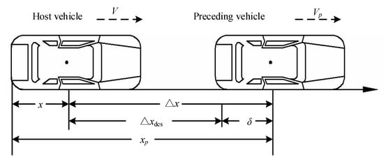
Figure 1.
Longitudinal kinematics for the adaptive cruise control (ACC) system.
The inter-distance error between the actual and desired inter-distance at time step k can be expressed as
with
where δ(k) represents the inter-distance deviation at time step k; δreal(k) represents the real inter-distance, and δtarget(k) represents the target inter-distance at time step k; x(k) and xp(k) represent the positions of the host vehicle and the preceding vehicle at time step k, respectively; do represents the minimum safety inter-distance between the host vehicle and the preceding vehicle at time step k, where the velocity of the host vehicle is low or zero; th represents the desired time headway, v(k) represents the velocity of the host vehicle.
Different from the constant time headway (CTH) strategy, the variable time headway (VTH) strategy is adopted, which considers the effects of the host vehicle velocity and the relative velocity between the host vehicle and the preceding vehicle. In our previous work, we verified the superior performance of VTH [18]. The desired time headway can be expressed as
where t1, t2, and t3 are positive constants, which can be approximated by the reaction time of the driver; vmax represents the maximum velocity of the host vehicle; and vrel(k) represents the relative velocity between the host vehicle and the preceding vehicle at time step k.
According to the discrete differential theory, the acceleration and jerk of the host vehicle at time step k can be represented as
where a(k) and j(k) represent the acceleration and the jerk of the host vehicle at time step k, respectively, and Ts is the sampling period of the ACC system.
Then, the relationship between the actual acceleration and the desired acceleration of the host vehicle satisfies the following conditions [19]:
where τ is the time lag of the ACC system, and u(k) is the desired acceleration at time step k.
According to the mutual longitudinal kinematics characteristics between the host vehicle and the preceding vehicle of the ACC system, the discrete kinematics equation can be expressed as
where ap(k) is the acceleration of the preceding vehicle at time step k.
3.2. Car-Following State Space Model
The dynamic characteristics of the ACC system should be considered when designing an ACC algorithm. Therefore, this paper regards the acceleration of the preceding vehicle as a disturbance to the ACC system. At the same time, to improve the robustness and control accuracy of the state space model, the dynamic characteristics of acceleration and jerk are also taken into account. For this purpose, this paper chooses the inter-distance Δx(k), the velocity of the host vehicle v(k), the relative velocity vrel(k), the acceleration of the host vehicle a(k), and the jerk of the host vehicle j(k) as the state variables of the prediction model, that is x(k) = [Δx(k), v(k), vrel(k), a(k), j(k)]T. The disturbance of the system is w(k) = ap(k). Then, the car-following state space model can be defined as
where the system matrices are
For the ACC system, safe car following is the required premise for designing the ACC strategy. While it can be achieved by ensuring a safe distance, two vehicles are likely to crash before achieving the desired safe distance. Therefore, the actual inter-distance between the preceding vehicle and the host vehicle must be restricted to ensure safety, yielding the first hard constraint
where dc is the minimum safe distance between the host vehicle and the proceeding vehicle.
The driver’s following behavior is to make the actual distance between the two vehicles close to the desired distance. At the same time, the velocity of the host vehicle is close to the velocity of the preceding vehicle. In other words, the two vehicles are relatively stationary, which means δ(k) and vrel(k) converge to zero in the steady state.
Riding comfort is another important requirement for designing an ACC system. Yi and Chung [20] researched the evaluation criterion for riding comfort by conducting surveys on a large number of drivers. The results indicate that vehicle acceleration and jerk can be used to describe the driving comfort of the vehicle. The smaller the absolute values of acceleration and jerk are, the better the ride comfort will be. Therefore, the velocity, the acceleration, the target acceleration, and the jerk of the host vehicle are limited to ensure riding comfort, which are defined as the following hard constraints:
where vmin, vmax, amin, amax, jmin, jmax umin, and umax are the bounds of the velocity, the acceleration, the desired acceleration, and the jerk, respectively.
The smoother the vehicle dynamic response curve is, the higher the vehicle fuel economy will be. Therefore, the reference trajectory is imported to make the variable that needs to be optimized gradually converge to the expected value, thus decreasing fuel consumption. The reference trajectories of inter-distance error, relative velocity, relative acceleration, and jerk are taken as the exponential attenuation functions; these are defined as
where δref(k + i), vrel_ref(k + i), aref(k + i), and jref(k + i) are the reference trajectories at step i in the predictive time domain for the inter-distance error, relative velocity, acceleration, and jerk, respectively; δtarget(k), vrel_des(k), ades(k), and jdes(k) are the desired inter-distance error, desired relative velocity, desired acceleration, and the desired jerk, respectively; and φ1, φ2, φ3, and φ4 are the damping exponents of reference trajectory for the inter-distance error, relative velocity, acceleration, and jerk, respectively.
The ACC system needs to satisfy the basic requirements for safety car following. Meanwhile, riding comfort and fuel economy are also important evaluation indexes. Therefore, this paper chooses the inter-distance error δ(k), relative velocity vrel(k), the acceleration a(k), and jerk of the host vehicle j(k) as the output variables of the prediction model, that is y(k) = [δ(k), vrel(k), a(k), and j(k)]T. The car-following output equation is
where
4. Multi-Objective ACC Strategy with Constraint Softening
A multi-objective ACC strategy based on MPC is designed in this section. Firstly, a prediction model is established based on a car-following state space model. Then, the objective functions for the ACC system are developed by introducing the system constraints for acceleration and jerk; the performance of the ACC system is also constructed. Finally, the constraint softening is conducted to enhance the convergence of the MPC optimization problem.
4.1. Prediction Model
The MPC algorithm can minimize the objective function by making full use of the model of the plant process. This can be done by utilizing a model to estimate the influence of control on the system output, which can then be reformed online [21]. On the basis of the system model and the current states of the system, the future states of the system can be predicted. To compensate for the predictive error and enhance the model accuracy, the feedback strategy can be utilized. On the basis of the state space model of car following, the predictive state variables in the predictive domain are calculated as
with
where p and c symbolize the predicted horizon and the control horizon, respectively. , , …, represent the estimated state values in the predicted horizon based on their values at the sampling time k; , , …, represent the estimated output values in the prediction horizon based on their values at the sampling time k; u(k), u(k + 1), …, u(k + c − 1) symbolize the control vectors, which represent the desired acceleration; w(k), w(k + 1), …, w(k + p) are the disturbance vectors in the predicted horizon; x(k) is the current state variable at the sampling time k, is the estimated value of the state variable for the sampling time k based on the previous sampling time k − 1; represents the deviation between the current state value and the estimated value at the sampling time k, which can be achieved using the function ; and , , , , , , are the prediction matrices, which are defined as
, are the error feedback matrices, which are defined as
At the sampling time k, the interference vector cannot be obtained. Therefore, this paper utilizes the acceleration of the host vehicle, as well as the relative velocity between the host vehicle and the preceding vehicle, to estimate the interference vector. Assuming that the perturbation value of the previous sampling time k − 1 stays the same within the predicted horizon, we can get the estimation of the perturbation vector at the sampling time k at the predicted horizon. It can be calculated as follows:
where represents the estimated perturbation value at the sampling time k based on that of the previous sampling time k − 1.
4.2. System Constraints
When designing the MPC optimization problem, the physical constraint of the system must be taken into account. The bounds of the desired acceleration are the most common constraints for the MPC problem. This paper limits the upper and lower bound of the desired acceleration by
where umin and umax represent the minimum and maximum values of the target acceleration of the host vehicle, respectively.
Limited by the physical condition of the ACC system, the change rate of the desired acceleration between each step cannot be infinite. Therefore, the change rate of the desired acceleration also has a bound, which is expressed by the following equation:
where Δumin and Δumax represent the minimum and maximum values of the target jerk. It can be transformed to the following equation:
Therefore, the desired acceleration constraint condition can be expressed as
To achieve the ideal performance of the ACC system, the inter-distance Δx(k), the velocity v(k), the acceleration a(k), and the jerk of the host vehicle j(k) are limited in this paper. Therefore, we define a new vector χ(k) = [Δx(k), v(k), a(k), j(k)]T and limit this vector at each step of the prediction space by
where χmin and χmax are the minimum and maximum values of the vector χ. χmin = [dc, vmin, amin, jmin]T and χmax = [inf, vmax, amax, jmax]T.
The above constraint can be rewritten as
with
According to the prediction model, the above performance constraint can be rewritten as
4.3. Objective Functions
Considering the change rate of the desired acceleration and making the control signal change smoothly, this paper takes the variation of the desired acceleration as the first control objective. The first control objective function can be expressed in the form of the least squares norm as
where s is the weight matrix of the desired acceleration variation.
According to the MPC algorithm, the aim of the controller is to minimize the error between the predicted output value and the reference output value. Therefore, the second objective function can be expressed in the form of the least squares norm as
where Yr is the reference output matrix and Q is the output weight matrix at each step of the predict horizon; fa = diag[φ1, φ2, φ3, φ4] is the reference output matrix of the first step; q = diag[q1, q2, q3, q4] is the output weight vector at each step; and q1, q2, q3, and q4 are the weight coefficients.
4.4. Constraints Softening
4.4.1. The Objective Function after Constraint Softening
Constraint softening is used to make the solution fall within the feasible region as far as possible. Soft constraints can be used as the output, which can limit the output holding inside the wanted boundaries. By constraining the softening method, we can add a penalty function to the objective function of the MPC problem [22], which can be expressed in the form of the least squares norm as
where is the slack variable of the input; is the penalty factor of the slack variable at the sampling step I; and sω is the weight matrix of the slack variables of each step.
After adding the penalty function, a new variable Ψ is added to the optimization variable. The new optimization variable is
By ignoring the useless items ρ1 and ρ2 of the first and the second objective functions, the objective function of the new optimization problem can be written as
4.4.2. The Constraints after Constraints Softening
As a result of importing the new optimization variable, the corresponding changes to the constraints of the original optimization problem should be made.
The new desired acceleration constraint can be written as
The new desired change rate of the acceleration constraint can be written as
After constraints softening, the new performance constraint can be achieved by the following constraints:
It can be rewritten as
Then, the new performance constraint is
According to the new objective function and constraints, the final optimization problem can be expressed as
The above optimization problem can be transformed into a standard quadratic programming (QP) problem, which can be calculated according to the active set method at each sampling time, by utilizing the Matlab optimization toolbox [23]. The first element of the solution of the quadratic programming problem is the desired acceleration control value.
5. Case Studies
The effectiveness of ADAS is usually assessed through simulation studies. Traditional vehicle models are mostly based on Matlab/Simulink, which need to set up complex simulation working conditions and driver models to complete the closed-loop operating mode simulation. Instead, this paper utilizes Matlab/Simulink and CarSim to verify the proposed ACC strategy in a more real transportation circumstance. CarSim has such advantages as a high precision and stable operation and it can set up a complete driver model. For comparison, the proposed multi-objective ACC strategy with constraint softening is represented by ACC-Soften. The ACC strategy proposed in [24] is represented by a multi-objective ACC algorithm (MO-ACC), which is based on the MPC algorithm, considering the car-following and economy performance. At the same time, the constant time headway was utilized to analyze the mutual longitudinal kinematics model. The results indicate their superiority as compared with the linear quadratic regulator (LQR)-based ACC algorithm (LQR-ACC). The performances of car following, safety, comfort, and economy were tested to validate the performance of the proposed ACC algorithm. The working condition of the preceding vehicle was set according to Figure 2.
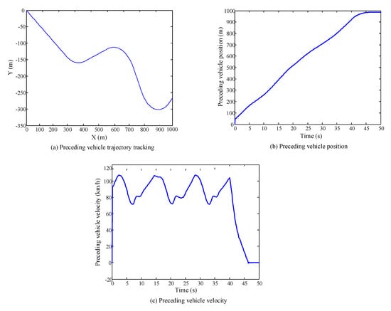
Figure 2.
The working condition of the preceding vehicle.
Figure 2a shows the running trajectory of the preceding vehicle in the Federal Highway Administration (FHWA) Alt 3 Road working condition, which can be set up in CarSim. To better compare the algorithm in [24], we set the simulation parameters to the same values. At the same time, Alt 3 Road FHWA in the vehicle simulation software CarSim was selected to simulate the straight and curve of an ideal dry road. The parameters were set by the system itself without modification. The adhesion coefficient of the road was set to the value of 0.85, which simulates a dry road surface and is close to a real road surface. The radius of curvature of the roads was set to the values of 155 m, 150 m, and 125 m, respectively, which can effectively simulate the tracking situation of an actual vehicle under the conditions of a curve of a road. In this condition, the host vehicle needs to accelerate and decelerate frequently. The time for the simulation was set to 50 s.
Figure 2b shows the location of the preceding vehicle in the Alt 3 Road FHWA condition. Before the simulation, the preceding vehicle is located 45 meters from the starting point. The host vehicle is located at the start point from the beginning. The velocity of the preceding vehicle is shown in Figure 2c. In order to verify the effectiveness of the proposed ACC algorithm, the velocity of the proceeding vehicle changes every 12 seconds. It changes dramatically from 30.6 m/s to 19.5 m/s during the first 40 seconds. Within the last 10 seconds, the preceding vehicle begins to brake increasingly. As a result, its velocity changes from 30.6 m/s to zero. The comparison results for ACC-Soften and MO-ACC are shown in Figure 3.
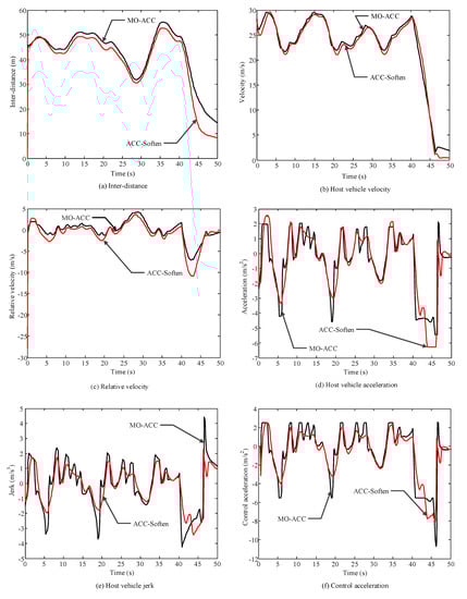
Figure 3.
Comparison results for ACC-Soften and multi-objective ACC algorithm (MO-ACC).
Figure 3a shows the response curve of the inter-distance. It can be seen that both ACC-Soften and MO-ACC can guarantee safety during car following effectively, keeping an inter-distance larger than the length of the vehicle body. This paper adopted the variable time headway strategy to analyze the mutual longitudinal kinematics model. Substituting the traditional constant time headway with the variable time headway can ensure driving safety and improve traffic flows in complex and changing traffic environments.
Figure 3b–d shows the velocity of the host vehicle, the relative velocity, and the acceleration of the host vehicle, respectively. Both ACC-Soften and MO-ACC can adjust the velocity to adapt to changes in the preceding vehicle, which helps to ensure the car-following performance. The velocity of the host vehicle with MO-ACC ranges between 21.98 m/s and 29.67 m/s and its acceleration ranges between −4.56 m/s2 and 2.05 m/s2 in response to the preceding vehicle; while the velocity of the host vehicle with ACC-Soften ranges between 21.07 m/s to 29.48 m/s and its acceleration ranges between −3.35m/s2 and 2.57m/s2 in response to the preceding vehicle. Compared with ACC-Soften, the variation range in terms of acceleration with MO-ACC shows that the host vehicle accelerates and decelerates more frequently during the first 40 s.
Figure 3e indicates that the maximum jerk for MO-ACC exceeds 3.70 m/s3. From Equations (3)–(5), the jerk can be determined by the actual acceleration and the desired acceleration. The controller is a process of optimizing and the rolling process. At the time interval around 45 s, the simulated actual acceleration for ACC-soften closely approximates a constant value, as can be seen in the Figure 3d. While the simulated desired acceleration for ACC-soften is not a constant value, as can be seen in the Figure 3f. According to Equation (5), jerk is determined by the actual acceleration and the desired acceleration and the jerk is not zero around 45 s. Researches indicate that the maximum absolute value of jerk suitable for passengers is 2.0 m/s3. Otherwise, the passengers will experience discomfort [25]. The average jerk values of ACC-Soften and MO-ACC are −0.2455 m/s3 and −0.2648 m/s3, respectively, which indicates that the ride comfort of ACC-Soften is 7.2% better compared with that of MO-ACC. During the emergent brake stage of the preceding vehicle for the last 10 seconds, both ACC-Soften and MO-ACC use larger braking acceleration to avoid collisions; whilst at the same time, comfort and economy are also guaranteed to a certain extent. The simulation results show that the driving comfort and the economy are drastically improved under the premise of ensuring safety and car following, at the same time, collision can be avoided with maximum braking acceleration when the preceding vehicle is in emergency braking.
The acceleration of the vehicle is closely related to the economic efficiency [26,27]. According to Figure 3d and Table 1, the average acceleration of ACC-Soften is −0.4849 m/s2, with a standard deviation of 2.024 m/s2 and range of 8.853 m/s2. The average acceleration of MO-ACC is −0.5072 m/s2, with a standard deviation of 2.056 m/s2 and range of 7.576 m/s2. Compared with MO-ACC, ACC-Soften has a lower acceleration standard deviation, without severe acceleration fluctuations. The economic efficiency of ACC-Soften is increased by 4.4% compared with that of MO-ACC.

Table 1.
Statistics of the acceleration of the host vehicle.
Figure 4 indicates that the average deviation between the actual inter-distance and the target inter-distance for MO-ACC is 2.698 m with a standard deviation of 3.757 m. The average deviation between the actual inter-distance and the target inter-distance for ACC-Soften is 1.116 m with a standard deviation of 2.536 m. This result shows that ACC-Soften can track the desired inter-distance better than MO-ACC.
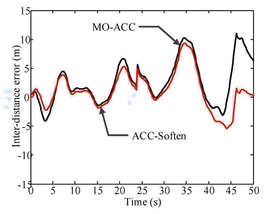
Figure 4.
Error of the inter-distance.
6. Conclusions
A multi-target adaptive cruise control strategy based on the model predictive control algorithm is proposed in this paper. When applying the MPC to design the controller, various problems can arise, such as a weak robustness, the solution being unfeasible, and high computational complexity. The constraint softening method is adopted to improve the robustness and to avoid the solution becoming unfeasible because of the overlarge feedback correction. Utilizing the MPC framework is helpful to deal with multiple objectives for automotive applications. By introducing the error analysis of the weight matrix, MPC is constructed as a closed-loop system to improve the accuracy of the system solution.
Simulations were conducted based on Matlab/Simulink and CarSim to verify the proposed ACC strategy in the FHWA Alt 3 Road condition. Two control strategies, ACC-Soften and MO-ACC, were compared to verify their performances in terms of car following, safety, comfort, and economy. The results indicate that the proposed ACC algorithm can improve the closed-loop convergence of MPC effectively and satisfy multiple control objectives. Constraint softening can be used to make the solution fall within the feasible region as far as possible. Compared with ACC-Soften, the variation range of acceleration with MO-ACC is larger. In this condition, the host vehicle needs to accelerate and decelerate more frequently, which results in discomfort of the passenger. Compared with MO-ACC, the proposed ACC-Soften control strategy shows a higher performance in terms of both comfort and economy when conducting safe car-following behavior.
In future work, the proposed ACC strategy will be validated to include a comparison with other recent methods. Furthermore, the experimental parameters may influence the feasibility and effectiveness of the algorithm to a certain extent. The road surface coefficient will affect the driving torque and then affect the acceleration of the controller. The curvature radius of the road will also affect the acceleration of the host vehicle whilst tracking the road. In future work, experiments will be conducted to analyze these influence. We also plan to apply the proposed algorithm to a real vehicle and combine the driver brake optimization switch to develop a better ACC strategy.
The main objectives in this paper focused on safety, car following, comfort, and economy, which were assessed under the framework of MPC. The proposed approach can serve as an upper controller to generate the desired acceleration, which can be applied to both electric vehicles and traditional vehicles with internal combustion engines to realize adaptive cruise control. The main purpose of this research was to enhance the active safety and intelligence of a distributed drive electric vehicle. Considering this application, in future, we hope to design a lower controller to distribute the desired torque for each wheel to achieve the desired acceleration.
Author Contributions
L.G. and P.G. conceived the idea of the study and conducted the research. Y.Q. analyzed most of the data and wrote the initial draft of the paper; L.G. and D.S. contributed to finalizing this paper. All authors have read and agree to the published version of the manuscript.
Funding
This research was funded by the National Natural Science Foundation of China, grant number 51975089 and 51575079; the China Postdoctoral Science Foundation, grant number 2018M641688; the Scientific Research Fund from the Education Department of Liaoning Province, grant number LJYT201915.
Conflicts of Interest
The authors declare no conflict of interest. The funders had no role in the design of the study; in the collection, analyses, or interpretation of data; in the writing of the manuscript, or in the decision to publish the results.
References
- Liu, H.; Wei, H.; Zuo, T.; Li, Z.; Yang, Y.J. Fine-tuning ADAS algorithm parameters for optimizing traffic safety and mobility in connected vehicle environment. Transp. Res. C-Emer. 2017, 76, 132–149. [Google Scholar] [CrossRef] [PubMed]
- Bengler, K.; Dietmayer, K.; Farber, B.; Maurer, M.; Stiller, C.; Winner, H. Three decades of driver assistance systems: Review and future perspectives. IEEE Intell. Transp. Syst. Mag. 2014, 6, 6–22. [Google Scholar] [CrossRef]
- Zhang, J.H.; Li, Q.; Chen, D.P. Integrated adaptive cruise control with weight coefficient self-tuning strategy. Appl. Sci. 2018, 8, 978. [Google Scholar] [CrossRef]
- Xiao, L.; Gao, F. A comprehensive review of the development of adaptive cruise control systems. Veh. Sys. Dyn. 2010, 48, 1167–1192. [Google Scholar] [CrossRef]
- Tordeux, A.; Lassarre, S.; Roussignol, M. An adaptive time gap car-following model. Transp. Res. B-Meth. 2010, 44, 1115–1131. [Google Scholar] [CrossRef]
- Shakouri, P.; Ordys, A.; Askari, M.R. Adaptive cruise control with stop&go function using the state-dependent nonlinear model predictive control approach. ISA Trans. 2012, 51, 622–631. [Google Scholar] [PubMed]
- Schmied, R.; Waschl, H.; Del Re, L. Comfort oriented robust adaptive cruise control in multi-lane traffic conditions. IFAC-PapersOnLine 2016, 49, 196–201. [Google Scholar] [CrossRef]
- Li, L.; Wang, X.; Song, J. Fuel consumption optimization for smart hybrid electric vehicle during a car-following process. Mech. Syst. Sign. Process. 2017, 87, 17–29. [Google Scholar] [CrossRef]
- Li, G.Q.; Gorges, D. Ecological adaptive cruise control and energy management strategy for hybrid electric vehicles based on Heuristic dynamic programming. IEEE Trans. Intell. Transp. 2019, 20, 3526–3535. [Google Scholar] [CrossRef]
- Khayyam, H.; Nahavandi, S.; Davis, S. Adaptive cruise control look-ahead system for energy management of vehicles. Expert Syst. Appl. 2012, 39, 3874–3885. [Google Scholar] [CrossRef]
- Luo, L.H.; Liu, H.; Li, P.; Wang, H. Model predictive control for adaptive cruise control with multi-objectives: Comfort, fuel-economy, safety and car-following. J. Zhejiang Univ.-Sci. A (Appl. Phys. Eng.) 2010, 11, 191–201. [Google Scholar] [CrossRef]
- Li, S.B.; Li, K.Q.; Rajamani, R.; Wang, J.Q. Model predictive multi-objective vehicular adaptive cruise control. IEEE Trans. Contr. Syst. Technol. 2011, 19, 556–566. [Google Scholar] [CrossRef]
- Gao, W.N.; Odekunle, A.; Chen, Y.F.; Jiang, Z.P. Predictive cruise control of connected and autonomous vehicles via reinforcement learning. IET Control Theory A 2019, 13, 2849–2855. [Google Scholar] [CrossRef]
- Shakouri, P.; Ordys, A. Nonlinear Model Predictive Control approach in design of Adaptive Cruise Control with automated switching to cruise control. Control Eng. Pract. 2014, 26, 160–177. [Google Scholar] [CrossRef]
- Zeilinger, M.N.; Jones, C.N.; Morari, M. Robust stability properties of soft constrained MPC. In Proceedings of the 49th IEEE Conference on Decision and Control, Atlanta, GA, USA, 15–17 December 2010; pp. 5276–5282. [Google Scholar]
- Li, S.E.; Xu, S.; Kum, D. Efficient and accurate computation of model predictive control using pseudospectral discretization. Neurocomputing 2016, 177, 363–372. [Google Scholar] [CrossRef]
- Naus, G.J.L.; Ploeg, J.; Van De Molengraft, M.J.G.; Heemels, W.P.M.H.; Steinbuch, M. Design and implementation of parameterized adaptive cruise control: An explicit model predictive control approach. Control Eng. Pract. 2010, 18, 882–892. [Google Scholar] [CrossRef]
- Guo, L.; Qiao, Y.F.; Ge, P.S.; Xu, L.N. Multi-objective adaptive cruise control strategy based on variable time headway. In Proceedings of the IEEE Intelligent Vehicles Symposium, Changshu, China, 26–30 June 2018; pp. 203–208. [Google Scholar]
- Bageshwar, V.L.; Garrard, W.L.; Rajamani, R. Model predictive control of transitional maneuvers for adaptive cruise control vehicles. IEEE Trans. Veh. Technol. 2004, 53, 1573–1585. [Google Scholar] [CrossRef]
- Yi, K.; Chung, J. Nonlinear brake control for vehicle CW/CA systems. IEEE-ASME Trans. Mech. 2001, 6, 17–25. [Google Scholar]
- Enang, W.; Bannister, C. Modelling and control of hybrid electric vehicles (A comprehensive review). Renew. Sust. Energ. Rev. 2017, 74, 1210–1239. [Google Scholar] [CrossRef]
- Zanoli, S.M.; Pepe, C. A constraints softening decoupling strategy oriented to time delays handling with Model Predictive Control. In Proceedings of the American Control Conference, Boston, MA, USA, 6–8 July 2016; pp. 2687–2692. [Google Scholar]
- Guo, L.; Ge, P.S.; Sun, D.C. Torque distribution algorithm for stability control of electric vehicle driven by four in-wheel motors under emergency conditions. IEEE Access 2019, 7, 104737–104748. [Google Scholar] [CrossRef]
- Eben Li, S.; Li, K.; Wang, J. Economy-oriented vehicle adaptive cruise control with coordinating multiple objectives function. Veh. Syst. Dyn. 2013, 51, 1–17. [Google Scholar] [CrossRef]
- Zhao, R.C.; Wong, P.K.; Xie, Z.C.; Zhao, J. Real-time weighted multi-objective model predictive controller for adaptive cruise control systems. Int. J. Aut. Tech. 2017, 18, 279–292. [Google Scholar] [CrossRef]
- Martinez, J.J.; Canudas-de-Wit, C. A safe longitudinal control for adaptive cruise control and stop-and-go scenarios. IEEE Trans. Contr. Syst. Technol. 2007, 15, 246–258. [Google Scholar] [CrossRef]
- Noei, S.; Sargolzaei, A.; Abbaspour, A.; Yen, K. A decision support system for improving resiliency of cooperative adaptive cruise control systems. Compl. Adapt. Syst. 2016, 95, 489–496. [Google Scholar] [CrossRef]
© 2020 by the authors. Licensee MDPI, Basel, Switzerland. This article is an open access article distributed under the terms and conditions of the Creative Commons Attribution (CC BY) license (http://creativecommons.org/licenses/by/4.0/).