Article

Binaural Rendering with Measured Room Responses: First-Order Ambisonic Microphone vs. Dummy Head

Institute of Electronic Music and Acoustics, University of Music and Performing Arts Graz, Inffeldgasse 10/III, 8010 Graz, Austria
*
Author to whom correspondence should be addressed.
Appl. Sci. 2020, 10(5), 1631; https://doi.org/10.3390/app10051631
Submission received: 11 January 2020 / Revised: 11 February 2020 / Accepted: 21 February 2020 / Published: 29 February 2020
(This article belongs to the Special Issue Sound and Music Computing -- Music and Interaction)

Abstract

:
To improve the limited degree of immersion of static binaural rendering for headphones, an increased measurement effort to obtain multiple-orientation binaural room impulse responses (MOBRIRs) is reasonable and enables dynamic variable-orientation rendering. We investigate the perceptual characteristics of dynamic rendering from MOBRIRs and test for the required angular resolution. Our first listening experiment shows that a resolution between 15 and 30 is sufficient to accomplish binaural rendering of high quality, regarding timbre, spatial mapping, and continuity. A more versatile alternative considers the separation of the room-dependent (RIR) from the listener-dependent head-related (HRIR) parts, and an efficient implementation thereof involves the measurement of a first-order Ambisonic RIR (ARIR) with a tetrahedral microphone. A resolution-enhanced ARIR can be obtained by an Ambisonic spatial decomposition method (ASDM) utilizing instantaneous direction of arrival estimation. ASDM permits dynamic rendering in higher-order Ambisonics, with the flexibility to render either using dummy-head or individualized HRIRs. Our comparative second listening experiment shows that 5th-order ASDM outperforms the MOBRIR rendering with resolutions coarser than 30 for all tested perceptual aspects. Both listening experiments are based on BRIRs and ARIRs measured in a studio environment.

1. Introduction

Typically, binaural rendering involves a convolution of source signals with measured or modeled head-related impulse responses (HRIRs) or binaural room impulse responses (BRIRs) and playback of the corresponding ear signals via headphones [1]. Both HRIRs and BRIRs implicitly contain the cues accessible to the human auditory system to perceive sound from a certain direction and distance, with a certain source width, envelopment, or spaciousness, cf. [2,3]. In order to reduce poor externalization when using both individual and non-individual HRIRs, it is often helpful to involve a natural or simulated acoustic room and thus to render with BRIRs instead. It is shown in [1,4] that BRIRs measured with a loudspeaker and a dummy head can achieve static binaural rendering of high audio quality and of convincing realism. Such a BRIR-based virtualization of loudspeakers in rooms is not only useful to virtualize multi-channel loudspeaker setups in mixing studios [5,6,7], but also to document and preserve acousmatic or electroacoustic music sceneries.
By involving the natural interaction of the ear signals with the head rotation of a listener, i.e., head-tracking [8] and dynamic rendering, immersion is improved as this reduces localization ambiguities and poor externalization [9,10,11]. Dynamic and interactive head-tracked BRIR rendering requires the acquisition of MOBRIRs (multi-orientation BRIRs), which can be tedious for highly resolved orientations. For best individualized results, in particular, one would need to measure MOBRIRs of each individual listener in each room to be auralized. Efficient and versatile alternatives [12,13,14] propose to measure the listener-dependent (HRIRs) and room-dependent (RIRs) parts separately to enable individualization as a second step.
State of the art: Linear interpolation of coarse-orientation MOBRIRs can cause strong comb-filter artifacts. Lindau [15] showed for multiple-orientation binaural recordings that the minimum required binaural grid resolution to avoid artifacts is most sensitive in anechoic conditions, and less sensitive reverberant cases, in which particular reverberation did not matter. To ensure continuous and robust interpolation from orientations coarser than 3 , a dual-band interpolation strategy is required, which literature refers to as motion-tracked binaural (MTB) [16]. At low frequencies, the dual-band approach interpolates the headphone signal from neighboring pairs of recorded ear signals linearly, while comb filters at high frequencies are avoided by combining interpolated spectral magnitudes with suitable phase values, e.g., found by spectrogram inversion [17]. Less challenging approaches yielding a suitable phase are discussed in [18] and perceptual properties are studied in [19]. Perceptually optimal cross-over frequencies and block sizes were investigated in [20] for the static and dynamic case, with which rendering from MOBRIRs resolved finer than 30 was found to be indiscernible from a 1 -resolved reference.
Dynamic rendering based on first-order Ambisonic RIRs (ARIRs) and a pre-measured set of high-resolution HRIRs, e.g., of a dummy head [21], is studied in [22]. Static rendering with ASDM (Ambisonic Spatial Decomposition Method) upscaling was shown to yield perceptually indistinguishable results for 7th order when compared to a reference dummy-head BRIR. Moreover, the study involved three rooms of different reverberation times (0.3 s, 0.7 s, and 1.4 s) and could show that the performance of the ASDM method did not depend on the particular reverberation time.
Contents: ARIR-based and MOBRIR-based rendering haven’t been compared yet, and our contribution deals with establishing a balanced comparison. The goal is to find out configurations in which both methods yield perceptually optimal or correspondingly scaled results. Some correspondence is expected, as both the binaural Ambisonic rendering of ARIRs using MagLS [22,23] and the interference-avoiding high-frequency strategy of MOBRIR-based rendering [20] rely on spectral phase simplification at high frequencies, and both relate to an angular resolution. To make the comparison reproducible, a room impulse response data set (dummy head and Ambisonic microphone) is measured in a studio environment and made accessible in this contribution. As the main part of the paper, Section 3 is dedicated to our comparative listening experiment on variable-orientation rendering from MOBRIRs resolved in { 30 , 45 , 60 } steps and corresponding ASDM-based Ambisonic orders { 5 , 3 , 1 } rendered using the same dummy head HRIRs [21].
As the Ambisonic renderer is already available (https://plugins.iem.at/), we dedicate Section 2 of the paper to supporting open research into MOBRIR-based rendering by providing an implementation example (Appendix A), example renderings (https://phaidra.kug.ac.at/view/o:77319), listening test response data (https://opendata.iem.at/projects/listening_experiment_data/), and a summarized statistical analysis of research presented at AES IIA [20].
In both listening experiments, participants are asked to rate for static rendering the perceptual attributes (i) timbre, (ii) spatial mapping, and for dynamic rendering (iii) its continuity. Both experiments compare the renderers to coarse linear MOBRIR interpolation (anchor) and to linear interpolation from 1 MOBRIRs (reference).
Measurements: The RIR measurements used here are available online (https://opendata.iem.at/projects/binauralroomresponses/) and were taken from the IEM production studio (volume 127 m 3 , base area 42 m 2 , T 60 0.4 s ) in which Neumann (Germany) KH310-A loudspeakers are mounted in various directions. MOBRIRs were measured with a Neumann KU100 dummy head in rotations of 1 steps (turntable) using the exponentially swept sine technique. Available loudspeaker directions that are depicted in Figure 1a, Figure 1b show the dummy head in the center listening position, facing the center loudspeaker (channel 3). The B-format ARIRs were measured after replacing turntable and dummy head with the Soundfield ST450 array. The room was selected for studying MOBRIR interpolation and binaural Ambisonic rendering as the presence of its short reverberation already supports externalization in typical listening environments and its pronounced direct and early parts are expected to be critical considering both timbral artifacts and spatial mapping deficiencies [15,24].

2. Experiment I: Dynamic Rendering of Multiple-Orientation Binaural Signals

Experiment I is based on data of a previous study [20], and it evaluates the dual-band strategy linear interpolation with switched high-frequency phase (LISHPh) using dummy-head MOBRIRs of the resolutions 8 , 15 , 30 , and 60 , and compares it with a reference linear interpolation of MOBRIRs resolved by 1 . The LISHPh method is described in Section 2.1, and the design and implementation of the listening experiment are discussed in Section 2.2 and Section 2.3, respectively. Response data (https://opendata.iem.at/projects/listening_experiment_data/) and examples of the audio stimuli (https://phaidra.kug.ac.at/view/o:77319) are made available for download; examples include renderings of static head-orientations and of emulated continuous head rotation. Finally, the results of Experiment I are discussed in Section 2.4.

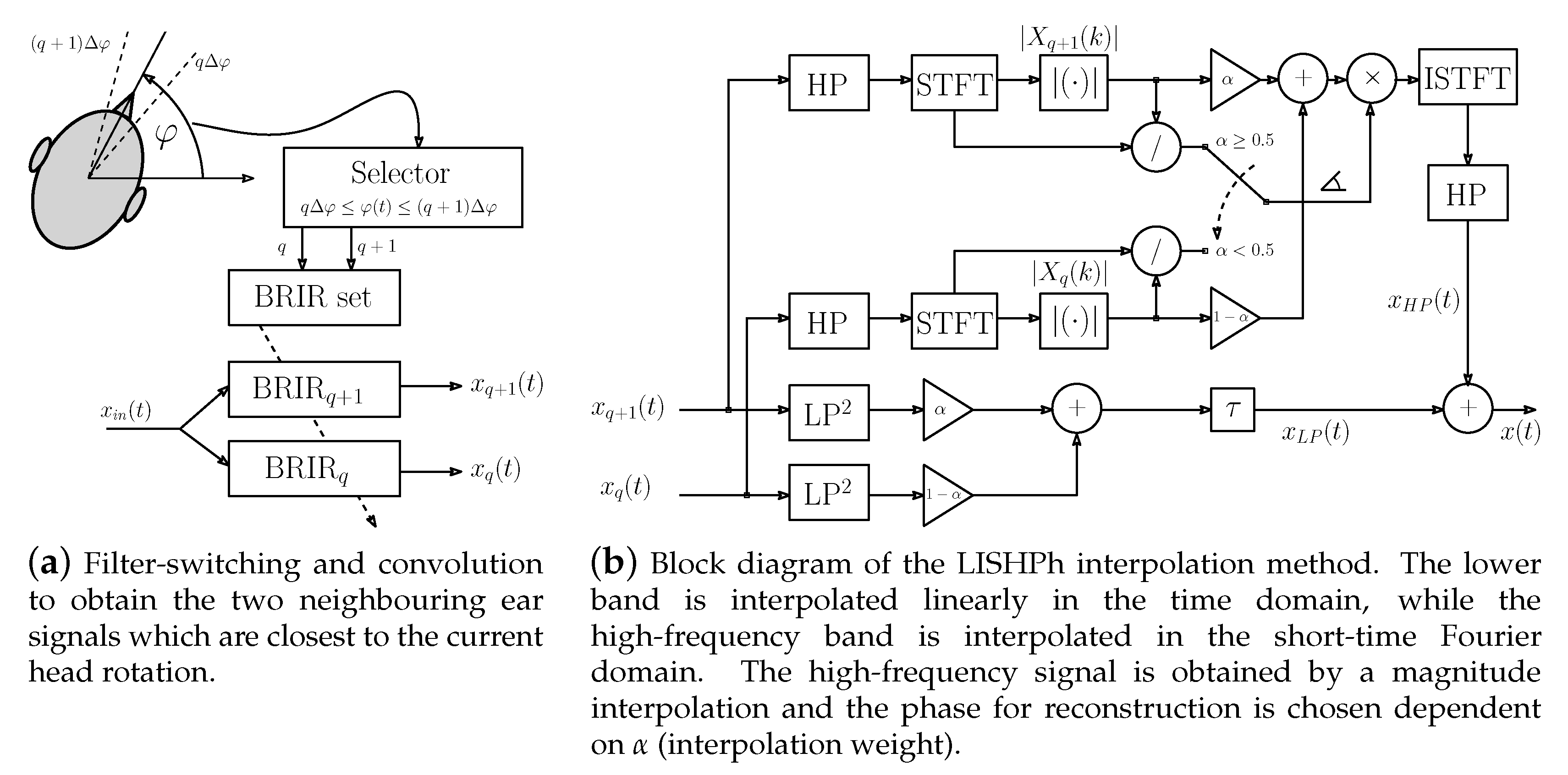
2.1. Linear Interpolation with Switched High-Frequency Phase (LISHPh)

For both the left and right ear, the interpolated ear signal in a horizontal set of orientations is obtained by a combination of the corresponding signals x q ( t ) and x q + 1 ( t ) belonging to the head orientation closest to the current orientation of the listener φ ( t ) , where t is the discrete-time index. With MOBRIRs measured for Q equi-angular orientations on the horizon (around the Cartesian z-axis), and Δ φ as azimuthal resolution, the indices of the two closest BRIRs (or recorded ear signals) are q = φ ( t ) Δ φ , and q + 1 = φ ( t ) Δ φ , where · and · are the floor and ceil functions, respectively, and the ear signals x q ( t ) , and x q + 1 ( t ) are obtained by convolution; see Figure 2a.
In a broadband linear interpolation, the resulting ear signal is obtained as
x ( t ) = ( 1 α ) x q ( t ) + α x q + 1 ( t ) ,
where the interpolation weight is obtained by α = φ ( t ) Δ φ φ ( t ) Δ φ . However, the linear combination of delayed signals produces comb-filtering introducing severe colorations in the resulting signal. In particular, the maximum delay τ = r c sin ( Δ ϕ ) between adjacent HRIRs is estimated by a simplistic head model, where r = 8.5 cm is the head radius and c = 343 m/s is the speed of sound. The maximum delay is observed between ear signals of the head orientation 0 and those of the orientations ± Δ φ , for a frontal source. To avoid destructive interference, artifact-free linear interpolation can only be achieved below
f m a x = 1 2 τ = c 2 r 1 sin ( Δ ϕ ) .
Spectral artifacts of linearly interpolated BRIRs are comparable with those of HRIRs when the direct sound dominates. For interpolation of BRIRs from a diffuse field, the same (worst-case) frequency limit for destructive interference holds. In particular, if the contribution of frontal sounds is pronounced, the interpolated result partly contains the destructive interference at f m a x .
The LISHPh method is employed [16,18,20] to avoid noticeable spectral artifacts around and above f m a x , regardless of the acoustic scenario. As depicted in Figure 2b, the signal in the lower band is processed in the time domain by applying the linear weights as in Equation (1), and the signal in the high-frequency band is obtained by magnitude interpolation
X ( k ) = { ( 1 α ) | X q ( k ) | + α | X q + 1 ( k ) | } e i ( k ) ,
where k is the frequency index of a short-time Fourier transform (STFT) frame, i 2 = 1 , and ( k ) is the phase argument which is switched between ( k ) = q + 1 ( k ) for α 0.5 and ( k ) = q ( k ) else. Whenever the phase argument of a narrow-band signals has to make a transition by π , switching can theoretically become audible and can only be avoided by spectrogram inversion [17,18]. We avoided the additional effort, as the negative influence of the switching noise turned out to be inaudible for speech, music recordings, noise, etc. with suitable block size settings [20].

2.2. Listening Experiment: Design

We tested the LISHPh method rendering from MOBRIR resolutions of Δ ϕ = { 8 , 15 , 30 , 60 } and also included the broadband linearly interpolated ear signals for comparison. During the listening experiment, each listener was asked to (i) rate the spatial mapping (i.e., direction and distance) and timbre compared to a reference condition for static rendering (four different head orientations), and (ii) to rate the continuity or robustness when rendering dynamically, i.e., incorporating head movements of the listener.
The 10 test participants (all male and at an age between 27 and 42) were asked to rate the overall difference between a reference (artifact-free linear interpolation with 1 resolution) and the test signals on a continuous scale from poor to very good. A hidden reference was used for screening of ratings, and thus the test procedure can be described as MUSHRA-like (multi stimulus with hidden reference and anchor [25]). The test signals were continuously looped, and participants were allowed to seamlessly switch between signals in real-time as often as desired.
In terms of timbre and spatialization, we tested four different static head orientations φ = { 12 , 21 , 37 , 78 } (the sign of the orientation was randomly changed across participants) for a frontal source position with pink noise and music as source signal, respectively. The choice of the source position and orientations was met to make the experiment most sensitive to the expected interpolation artifacts: on the one hand, time-delays (phases or ITDs) are most head-orientation-dependent for predominantly frontal source positions, and, on the other hand, orientations were selected to enforce interpolation with 0.2 < α < 0.8 for all MOBRIR sets under test.
Testing the continuity involved a pink noise and a music signal played back over a virtual frontal ( 0 ) and lateral ( 90 ) loudspeaker. Here, listeners were asked to rotate their head between ϕ = 45 45 and a check-box for automatic rotation with 180 / 1 s was included for fast movements.

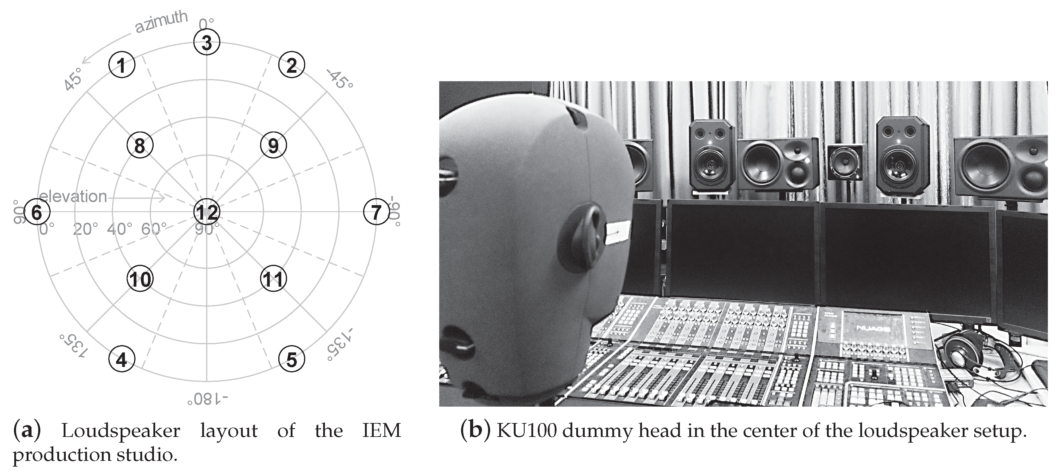
2.3. Listening Experiment: Implementation and Settings

The real-time implementation of the LISHPh, as well as the broadband linear interpolation, was done in pure data (https://puredata.info/), an open source real-time audio software. Appendix A describes the example implementation provided online (https://phaidra.kug.ac.at/o:97087).
Block processing: In the short-time block processing with block size N and hop size L = N / 2 of the high-frequency part, a sine half-wave window is applied at both the analysis and synthesis stage to reduce cyclic artifacts at the block boundaries. As found in [20] and as the optimum for broadband musical sounds, it is crucial to keep the block size low to avoid temporal artifacts and to obtain low latency. Thus, we suggest setting N = 128 at a sampling rate of 44.1 kHz. For high-frequency phase selection, we used an update rate of 200 Hz; see the block labeled as Selector in the diagram of Figure 2a.
Crossover: We estimate the spectral ripple of two interfering signals with phase offsets by 1 2 [ e i ϕ 2 + e i ϕ 2 ] = cos ϕ 2 . To keep the spectral ripple below 3 dB, we require a phase difference ϕ < π 2 , or ϕ < π 4 to keep it below 0.7 dB, and hence spectrally inaudible [26]. With Equation (2) or a rule of thumb f m a x 2 kHz 57.3 Δ φ , the phase difference is ϕ = π f f m a x in our case. Spectrally, good results are achieved with a crossover frequency f c f m a x 4 . However, setting it too low, e.g., f c < 1.5 kHz, impedes interaural phase cues in a relevant frequency range. Accordingly, the choice
f c ( Δ ϕ ) = 2 u f m a x ( Δ ϕ ) ,
with u = 2 , if Δ φ < 30 1 , if Δ φ 30
offers a reasonable trade-off, cf. [20]. For Δ ϕ = { 8 , 15 , 30 , 60 } , we obtain the crossovers at f c = [ 4 , 2 , 2 , 1 ] kHz. The crossover is implemented by 4th-order Linkwitz–Riley filters because of their in-phase sub bands [27,28].
For playback, we used AKG K702 headphones equipped with the IEM headtracker [8] and the experiment was conducted in a quiet office room.

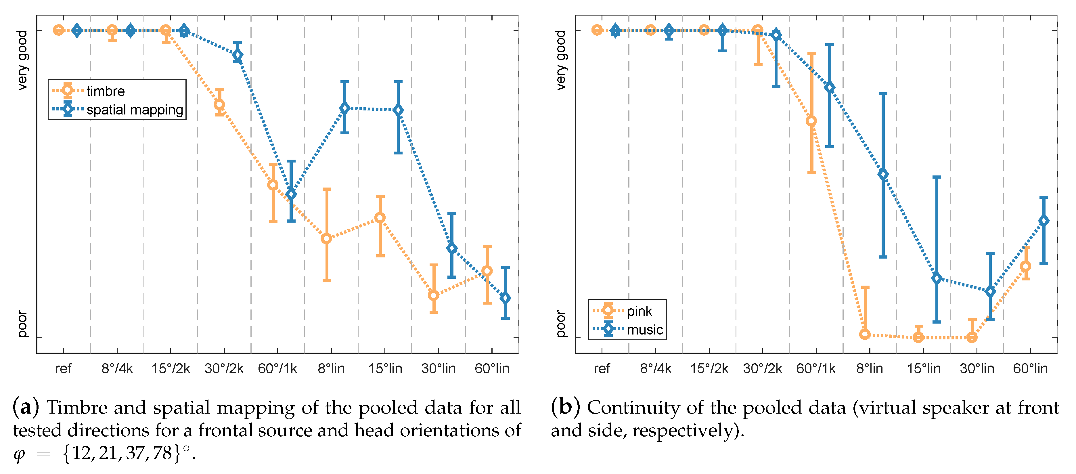
2.4. Results and Discussion

The statistical analysis below uses pooled data for each attribute; see Figure 3. For timbre and spatial mapping, ratings of four directions were pooled, and both virtual loudspeaker directions were pooled for continuity. Please note that throughout the article we use a Wilcoxon signed-rank test [29] with a Bonferroni–Holm correction [30] to determine p-values of pair-wise comparisons between test conditions and define p < 0.05 as significantly different. We employ non-parametric statistics as we do not assume a normal distribution of the ratings due to severe clustering at the limits of the scale.
Timbre: Per MOBRIR resolution, there is a clear advantage of the LISHPh method in the settings proposed compared to broadband linear interpolation. The p-values (significance level) given in the upper triangle of Table 1 indicate that there are four groups, which are significantly different from each other. The LISHPh interpolations with settings 8 /4k and 15 /2k are not significantly different ( p = 0.11 ) to the 1 reference condition and perform significantly better than all other conditions. For the coarser resolutions, the quality of the LISHPh interpolation decreases significantly with spacing. However, for all orientation resolutions, LISHPh performs significantly better than linear interpolation ( p < 0.005 ). The best linear interpolation conditions 8 lin and 15 lin are comparable to the worst LISHPh condition 60 /1k ( p > 0.36 ).
Spatial Mapping: The results for spatial mapping, i.e., localization and distance impression, indicate that there is no significant difference between the ref and 8 /4k, and 15 /2k ( p > 0.13 ) conditions, cf. lower triangle in Table 1. For coarser resolutions, the quality of spatial mapping decreases significantly. Again, the LISHPh conditions clearly outperform the linear interpolation. However, the best linearly interpolated conditions 8 lin and 15 lin are significantly better than the worst LISHPh condition 60 / 1 k. This is caused by its low crossover frequency at f c = 1 kHz which is set to avoid comb filtering (cf. Equation (5)) but already distorts the interaural time difference (ITD) in a sensitive frequency range [31].
Continuity: The results for perceived continuity are depicted in Figure 3b. While there is clear absolute difference depending on the source signal (yellow vs. blue line-pink noise vs. music), the trend is similar. For both signal types, all of the LISHPh conditions except 60 / 1 k do not significantly differ from the reference and from each other; see Table 2. Coarser MOBRIR resolutions lead to a decrease in quality, and LISHPh conditions clearly outperform linear interpolation of corresponding resolution. The improved continuity for 60 lin compared to the denser MOBRIRs can be explained by its reduced timbral variation when rotating the head, which seemed more important to listeners than spatial mapping.

3. Experiment II: Dummy-Head MOBRIR vs. ARIR

In Experiment II, we evaluate and compare the perceptual aspects of MOBRIR (LISHPh) and ARIR-based dynamic rendering (ASDM). The concept of ARIR-based rendering and the relevant signal processing involved to accomplish upscaling are described in Section 3.1. A description of the listening experiment, the implementation, and the corresponding discussions are presented in Section 3.2, Section 3.3 and Section 3.4, respectively. Appendix B shows the MATLAB implementation of the ASDM upscaling. Audio examples (https://phaidra.kug.ac.at/view/o:77319) of the material used in the listening experiment as well as its response data (https://opendata.iem.at/projects/listening_experiment_data/) are available for download. The examples include renderings of static head-orientations and of emulated continuous head-orientations.

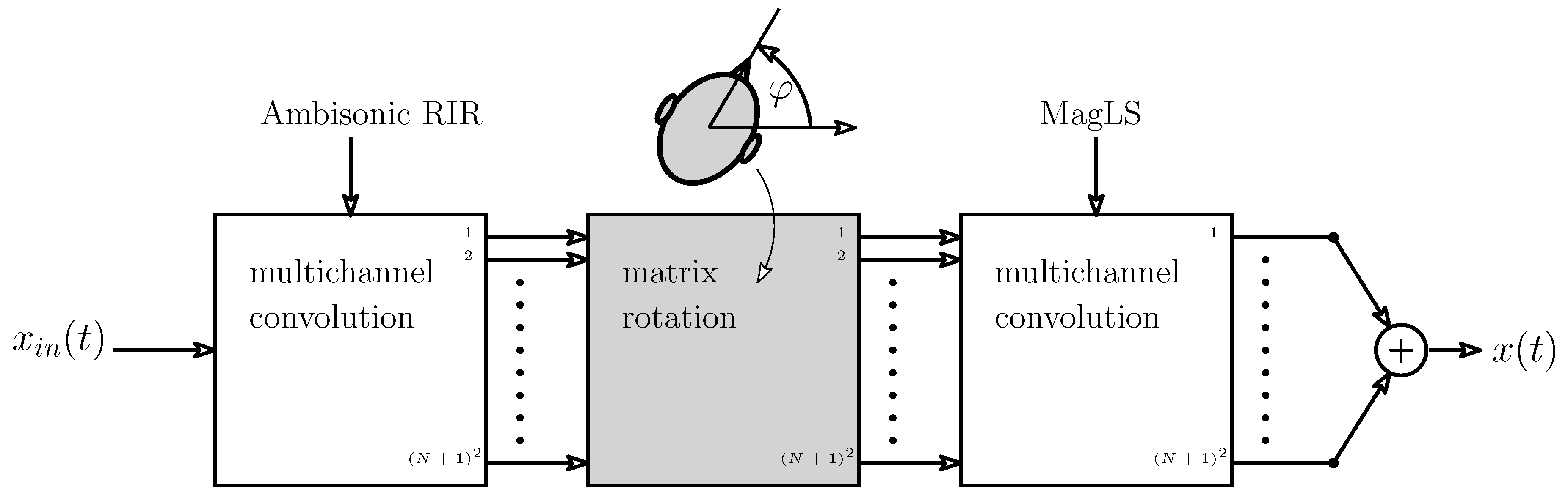
3.1. Rendering with Measured Ambisonic RIR and the Ambisonic Spatial Decomposition Method (ASDM)

As depicted in Figure 4, dynamic binaural rendering from room responses measured in Ambisonics (ARIRs) is modular and consists of three blocks: (i) a multi-channel convolution of the source signal with an order N upscaled ARIR, (ii) an efficient rotation [32,33] corresponding to the head orientation of the listener, (iii) and multi-channel convolution with an Ambisonic binaural renderer.
For efficient and low-effort measurements of the ARIR, we use a compact first-order tetrahedral spherical microphone array and denote the discrete-time B-format ARIRs h ( t ) , x ( t ) , y ( t ) , z ( t ) as the responses of a Soundfield ST450 array.
Similar to the spatial decomposition method SDM [34], the Ambisonic SDM (ASDM) assigns a direction of arrival (DOA) θ ( t ) to each discrete-time sample t of the omni-directional RIR component h ( t ) , cf. [22]. For the DOA estimation, we suggest using the pseudo-intensity vector (PIV) [35] for the frequencies between 200 Hz and 3 kHz . Here, the upper frequency limit is chosen below the spatial aliasing frequency f a = c 2 π r S T 450 3.6 kHz for r S T 450 = 1.5 cm and the low cut minimizes low-frequency disturbance in the DOA estimation. We perform a zero-phase band limitation (e.g., by MATLAB’s filtfilt) denoted by F 200 3 k and a zero-phase temporal smoothing F L of the resulting PIV using a moving-average Hann window in the interval [ L / 2 ; L / 2 ] for L = 16 to get the DOA estimate
θ ( t ) = θ ˜ ( t ) θ ˜ ( t ) , with θ ˜ ( t ) = F L F 200 3 k h ( t ) F 200 3 k x ( t ) y ( t ) z ( t )
as Cartesian unit vector θ ( t ) .
In a first step, the ASDM-upscaled ARIR re-encodes every time sample at the detected DOA
h ˜ n m ( t ) = Y n m [ θ ( t ) ] h ( t ) ,
where Y n m ( θ ) are the N3D-normalized, real-valued spherical harmonics of order n and degree m, cf. [23], evaluated at the direction θ , and the maximum order n N can be chosen freely. In the late diffuse part of the response, the implicit assumption of there being only a single DOA per time sample does not hold. As a result, a fluctuation of the DOA θ ( t ) causes amplitude modulation and destroys narrow-band spectral content in h ˜ n m ( t ) ; typically, the longer low-frequency reverberation tails are hereby mixed towards higher frequencies, causing unnaturally long reverberation there [12,36] at high orders, cf. solid lines in Figure 5. However, theoretically, the expected temporal energy decay in an ideal (isotropic) diffuse field must be identical for any receiver of random-energy-efficiency-normalized directivity, such as the spherical harmonics, also after decomposition into frequency bands, and hence requires correction.
Despite the mismatch, formal derivation in [22] showed that quadratic summation across same-order spherical harmonics is omnidirectional m | Y n m ( θ ) | 2 = 2 n + 1 4 π . Hereby, ASDM-upscaled ARIRs at least displays consistent broadband energies m | h ˜ n m ( t ) | 2 = 2 n + 1 4 π | h ( t ) | 2 across all spherical harmonic orders n, for any sound field. To enforce consistency with spectral squares of h ( t ) , third-octave filtering is useful, where the bth sub-band signal F b { h ( t ) } with center frequency f b is obtained from a bank of zero-phase filters F b that is perfectly reconstructing h ( t ) = b F b { h ( t ) } . For every sub band b and order n, an energy decay of the ASDM-upscaled ARIR F b { h ˜ n m ( t ) } matching with the original one of F b { h ( t ) } is enforced by envelope correction
F b { h n m ( t ) } = F b { h ˜ n m ( t ) } w n b ( t ) , with w n b ( t ) = 2 n + 1 4 π F T F b { h ( t ) } 2 m F T F b { h n m ( t ) } 2 ,
where F T { · } denotes temporal averaging with a time constant T (e.g., 100 ms). The energy decay reliefs for the initial and corrected result of ASDM are exemplary shown for a third octave f b = 2 kHz and within the orders n = { 1 , 3 , 5 , 7 } in Figure 5.
Finally, the ear signals are obtained by a convolution of the rotated Ambisonic signals with any state-of-the-art FIR binaural Ambisonic renderer, cf. Figure 4. Our study employs the time-invariant filters of the MagLS (magnitude-least-squares) renderer (The MagLS renderer is part of the IEM plugin suite which can be found here (https://plugins.iem.at/) defined in [24,37] to get high-quality Ambisonic rendering already with an order N = 3 . The filters were designed using a magnitude-learst-squares optimization that disregards phase match in favor of an improved HRTF magnitude at high frequencies, and hereby avoids spectral artifacts. MagLS also includes an interaural covariance correction that offers an optimal compromise to render diffuse fields consistently [23].

3.2. Listening Experiment: Design

Similar to Experiment I, listeners were asked to rate the spatial mapping, coloration, and continuity compared to the 1 reference. The test conditions included ARIR rendering with the ASDM target orders N = { 1 , 3 , 5 } as well as the corresponding MOBRIR resolutions Δ φ = { 60 , 45 , 30 } rendered with LISHPh and broadband linear interpolation. Note that the set of MOBRIR resolutions is derived from the number of loudspeakers used for Ambisonics reproduction [23] in practice Δ φ N 180 N + 1 ; for N = 1 , we chose 60 instead of 90 to maintain a reasonable MOBRIR resolution.
We asked to rate the timbre differences, and consistency of spatial mapping for the five static listener orientations φ = { 0 , 35 , 12 , 15 , 22.5 } which were switched automatically in 900 ms intervals and are restarted at the beginning of every audio loop. The orientations where chosen such that 0.25 < α < 0.83 for all resolutions in order to test for high interpolation depth; φ = 0 is included as reference orientation, and it marks the start of each loop. As source positions, we used a frontal and lateral virtual loudspeaker, cf. loudspeakers 3 and 7 in Figure 1a. The continuity test to compare dynamic rendering was similar as in Experiment I; see Section 2.2.

3.3. Listening Experiment: Implementation

While ARIR-based rendering could be implemented in a multichannel DAW (e.g., Reaper) by using freely available convolution (http://www.matthiaskronlachner.com/?p=1910), rotation, and rendering plug-ins (https://plugins.iem.at/), there is no tested and easy-to-use plug-in for MOBRIR rendering, yet. To rule out any effects due to different implementations, we used the pure data implementation as described in Section 2.3 to also emulate ARIR-based rendering. To this end, we evaluated the ARIR BRIRs according to [22] to get a Δ φ = 1 MOBRIR (for each ear)
A M O B R I R q ( t ) = τ = 0 T 1 n = 0 N m = n n b n m ( τ ) m = n n r n m m ( q Δ φ ) h n m ( t τ ) ,
where b n m ( t ) is the FIR binaural Ambisonic renderer, h n m ( t ) is the ARIR of the order N, q is the orientation index, and r n m m is the Ambisonic rotator. As binaural renderer b n m ( t ) , we employed the one from [37] with KU100 HRIRs measured for 2702 directions [21]. The resulting AMOBRIR was linearly interpolated like the reference condition.
For playback, we again used AKG K702 headphones equipped with the IEM headtracker [8] and the experiment was conducted in a quiet office room.

3.4. Results and Discussion

The results of the listening experiments with nine participants (all male experienced listeners with normal hearing, and between an age of 27 and 57) are depicted in Figure 6 and are discussed in detail below.
Timbre: While most of the conditions are rated significantly poorer than the reference, the following are not: LISHPh with 30 / 2 k and ARIR rendering with the ASDM-upscaled orders 3 and 5, cf. upper triangle in Table 3. ARIR rendering with 5th order is generally rated best; however, it is not significantly different to the 30 / 2 k and 3rd-order conditions. The timbral quality decreases with both orientation resolution and lower order, and thus the 60 / 1 k and 1st-order conditions yield significantly lower quality. The broadband linear interpolation conditions received the poorest ratings and significantly differ from all other conditions, with the exception of 60 / 1 k and 1st order.
Spatial Mapping: While the general trend is similar to the timbre results, for spatial mapping only the 1st order and all linear interpolations are significantly poorer than the reference, cf. lower triangle in Table 3. Again, the 5th-order ARIR rendering is rated highest, albeit not significantly better than the 3rd-order ARIR and all LISHPh conditions ( p > 0.68 ). The 30 , 45 , and 60 linear interpolations are significantly outperformed by all other conditions except the 1st-order ARIR rendering. Please note that we tested static directions different from Experiment I and even though the trend is similar to Figure 3a, the 30 / 2 k is not significantly different from the reference condition here. This can be addressed to participants not always rating the reference highest in Experiment II.
Continuity: The ratings of the continuity, i.e., robustness of source position and timbre to head rotations, are depicted in Figure 6b and Table 4, respectively. Tendentially, quality ratings are higher for music compared to pink noise as source signal. Independent of the source signal, the 5th-order and 3rd-order ARIR conditions as well as all LISHPh conditions do not significantly differ from the reference condition ( p > 0.15 ). Again, all linearly interpolated conditions and the 1st-order condition perform poorly, are significantly different to all other conditions, and are similar to each other.

4. Conclusions

We evaluated two fundamentally different measurement-based binaural audio rendering strategies in a novel comparative listening experiment: The dummy-head-based strategy employs binaural impulse responses measured in multiple orientations (MOBRIRs) and hereby contains the required set of binaural cues of the dummy head for dynamic (head-tracked) rendering. The Ambisonics-based strategy uses the room impulse response measured by a first-order Ambisonic microphone (ARIR) in a single orientation, which is upscaled from its weak directional resolution to higher orders using the Ambisonic spatial decomposition method (ASDM). Dynamic binaural rendering is then accomplished separately through an Ambisonic rotator and binaural renderer.
Our experiment successfully compared the perceptual performance of both strategies, for static rendering in terms of timbre and spatial mapping, and for dynamic rendering concerning the resulting temporal continuity, overall. We found that the 5th-order Ambisonics-based rendering strategy (ASDM) outperformed the dummy-head-based rendering for resolutions coarser than 30 . By this and by its clear separation of room-related from head-related aspects, we consider ASDM binaural rendering as the versatile high-quality option for dynamic binaural rendering based on measured room responses. We published audio examples, an example implementation, and all experimental response data for reproducible research.
Concerning the dummy-head-based strategy with MOBRIRs, we summarized the analysis and made available all experimental response data from previous experiments [20]. The results indicate that linear interpolation between the different dummy-head orientations is always outperformed by the linear interpolation and switched high-frequency phase method (LISHPh). This processing strategy achieved a convincing rendering quality with an orientation resolution of 15 and 30 , when compared to a 1 linearly interpolated reference.
The underlying RIR measurements were taken from the IEM production studio with a reverberation time of T 60 0.4 s . This specific choice of room was found suitable to study the MOBRIR interpolation and ASDM binaural rendering as its pronounced direct and early parts are expected to be critical considering specific timbral or spatial mapping deficiencies, and its reverberation is suitable to evoke externalized impressions in typical office environments. Note that neither of the investigated rendering strategies was specifically optimized for the specific room and signals. Although not formally tested, we assume the results to hold for a variety of other acoustic environments. An example patch and a set of more reverberant BRIRs (RT = 2.8 s) are provided online (https://phaidra.kug.ac.at/o:100863).

Author Contributions

Conceptualization, M.Z. and F.Z.; Writing—Original Draft Preparation M.Z. and F.Z. with periodic contributions by M.F.; Writing—Review & Editing, M.Z. and F.Z.; Software, M.Z. with periodic contributions by F.Z.; Listening Experiment Implementation, F.Z. and M.Z. with periodic contributions by M.F.; Listening Experiment Design, M.Z., M.F., and F.Z.; Data Analysis, M.F. and M.Z.; Measurements, M.Z. and F.Z. All authors have read and agreed to the published version of the manuscript.

Funding

This research received no external funding.

Acknowledgments

The authors thank all listeners for their participation in the listening experiment.

Conflicts of Interest

The authors declare no conflict of interest.

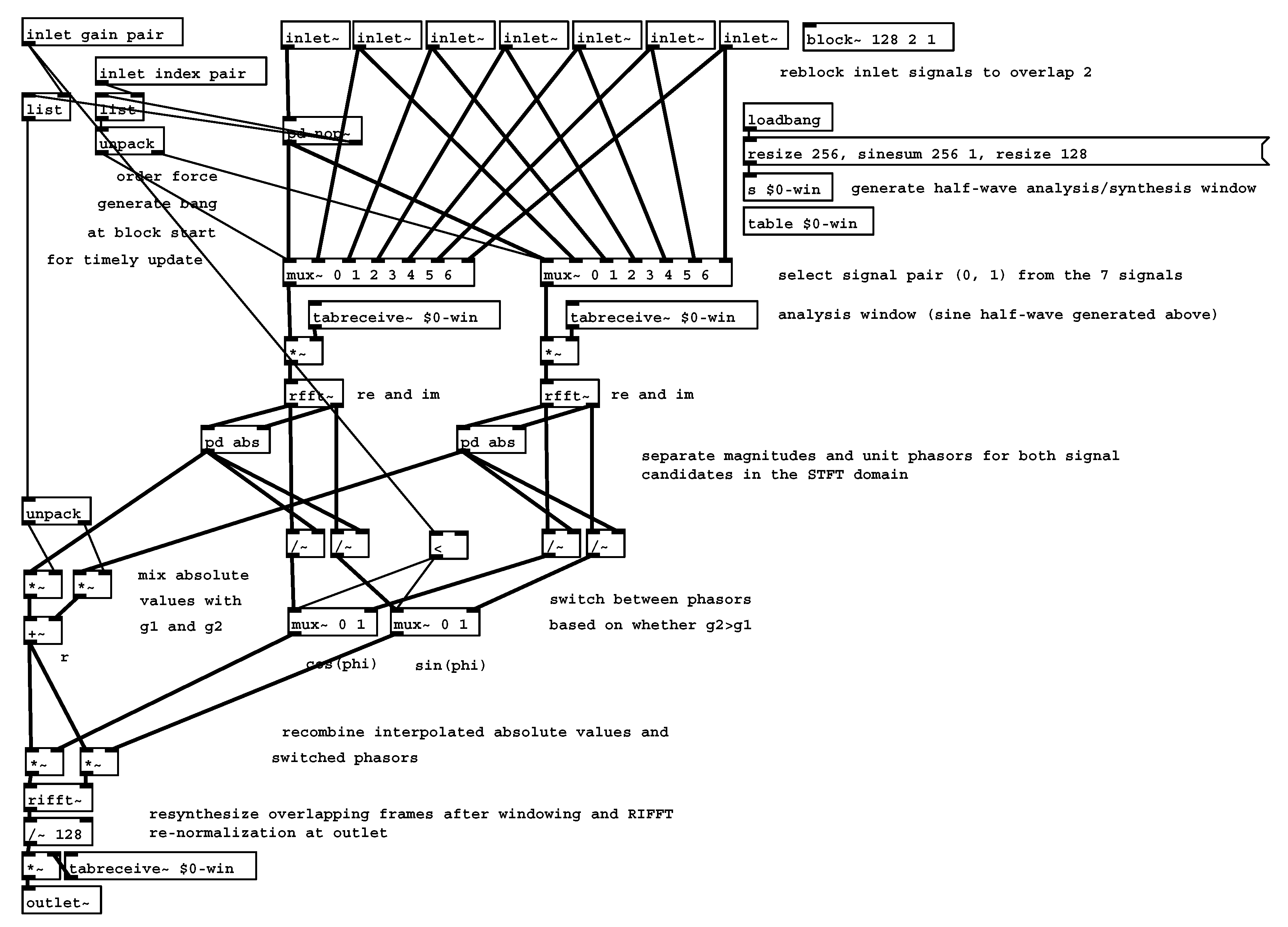
Appendix A. MOBRIR PureData Real-Time Processing Patch

An example patch for the pure-data real-time processing environment using M = 7 orientations with a resolution of Δ ϕ = 15 can be accessed here https://phaidra.kug.ac.at/o:97087. The patch for the high-frequency processing is exemplary shown for seven orientations in Figure A1.
Figure A1. Implementation of the high-frequency patch in Pd.
Applsci 10 01631 g0a1

Appendix B. ASDM MATLAB Source Code

The MATLAB source code of the proposed ASDM method can be found in Listing 1. Please note that you need to install the spherical harmonic transform which can be accessed from https://github.com/polarch/Spherical-Harmonic-Transform.
Listing 1. MATLAB source code of the proposed ASDM method.
Applsci 10 01631 i001

References

  1. Møller, H. Fundamentals of binaural technology. Appl. Acoust. 1992, 36, 171–218. [Google Scholar] [CrossRef] [Green Version]
  2. Pollack, I.; Trittipoe, W. Binaural listening and interaural noise cross correlation. J. Acoust. Soc. Am. 1959, 31, 1250–1252. [Google Scholar] [CrossRef]
  3. Okano, T.; Beranek, L.L.; Hidaka, T. Relations among interaural cross-correlation coefficient (IACCE), lateral fraction (LFE), and apparent source width (ASW) in concert halls. J. Acoust. Soc. Am. 1998, 104, 255–265. [Google Scholar] [CrossRef] [PubMed]
  4. Lindau, A. Binaural Resynthesis of Acoustical Environments-Technology and Perceptual Evaluation. Ph.D. Thesis, TU Berlin, Berlin, Germany, 2014. [Google Scholar]
  5. Smyth, S.M. Personalized Headphone Virtualization. U.S. Patent 7,936,887, 3 May 2011. [Google Scholar]
  6. Smyth, S.; Smyth, M.; Cheung, S. Headphone Surround Monitoring for Studios. In Proceedings of the Convention of the Audio Engineering Society, London, UK, 9 April 2008; pp. 1–7. [Google Scholar]
  7. Satongar, D.; Lam, Y.W.; Pike, C. Measurement and Analysis of a Spatially Sampled Binaural Room Impulse Response Dataset. In Proceedings of the 21st International Congress on Sound and Vibration, Beijing, China, 13–17 July 2014; pp. 1–8. [Google Scholar]
  8. Romanov, M.; Berghold, P.; Rudrich, D.; Zaunschirm, M.; Frank, M.; Zotter, F. Implementation and evaluation of a low-cost head-tracker for binaural synthesis. In Proceedings of the Convention of the Audio Engineering Society, Berlin, Germany, 20–23 May 2017. [Google Scholar]
  9. Begault, D.R.; Wenzel, E.M.; Anderson, M.R. Direct Comparison of the Impact of Head Tracking, Reverberation, and Individualized Head-Related Transfer Functions on the Spatial Perception of a Virtual Speech Source. J. Audio Eng. Soc. 2001, 49, 904–916. [Google Scholar] [PubMed]
  10. Brungart, D.S.; Kordik, A.J.; Simpson, B.D. Effects of headtracker latency in virtual audio displays. J. Audio Eng. Soc. 2006, 54, 32–44. [Google Scholar]
  11. Hendrickx, E.; Stitt, P.; Messonnier, J.C.; Lyzwa, J.M.; Katz, B.F.; de Boishéraud, C. Influence of head tracking on the externalization of speech stimuli for non-individualized binaural synthesis. J. Acoust. Soc. Am. 2017, 141, 2011–2023. [Google Scholar] [CrossRef] [PubMed] [Green Version]
  12. Zaunschirm, M.; Baumgartner, C.; Schörkhuber, C.; Frank, M.; Zotter, F. An Efficient Source-and-Receiver-Directional RIR Measurement Method. In Proceedings of the Fortschritte der Akustik-DAGA, Kiel, Germany, 6–9 March 2017; pp. 1343–1346. [Google Scholar]
  13. Pörschmann, C.; Wiefling, S. Perceptual Aspects of Dynamic Binaural Synthesis based on Measured Omnidirectional Room Impulse Responses. In Proceedings of the International Conference on Spatial Audio, Seattle, WA, USA, 26–30 May 2015. [Google Scholar]
  14. Menzer, F. Binaural Audio Signal Processing Using Interaural Coherence Matching. Ph.D. Thesis, EPFL, Lausanne, Switzerland, 2010. [Google Scholar]
  15. Lindau, A.; Maempel, H.J.; Weinzierl, S. Minimum BRIR grid resolution for dynamic binaural synthesis. J. Acoust. Soc. Am. 2008, 123, 3498. [Google Scholar] [CrossRef]
  16. Algazi, V.R.; Duda, R.O.; Thompson, D.M. Motion-tracked binaural sound. J. Audio Eng. Soc. 2004, 52, 1142–1156. [Google Scholar]
  17. Pruša, Z.; Balazs, P.; Søndergaard, P.L. A Non-iterative Method for STFT Phase (Re)Construction. IEEE/ACM Trans. Audio Speech Lang. Process. 2016, 25, 1154–1164. [Google Scholar] [CrossRef] [Green Version]
  18. Hom, R.C.M.; Algazi, V.R.; Duda, R.O. High-Frequency Interpolation for Motion-Tracked Binaural Sound. In Proceedings of the Convention of the Audio Eng. Soc. 121, San Francisco, CA, USA, 5–8 October 2006. [Google Scholar]
  19. Lindau, A.; Roos, S. Perceptual evaluation of discretization and interpolation for motion-tracked binaural (MTB) recordings. In Proceedings of the 26th Tonmeistertagung, Leipzig, Germany, 25–28 November 2010; pp. 680–701. [Google Scholar]
  20. Zaunschirm, M.; Frank, M.; Franz, Z. Perceptual Evaluation of Variable-Orientation Binaural Room Impulse Response Rendering. In Proceedings of the Conference of the Audio Eng. Soc.: 2019 AES International Conference on Immersive and Interactive Audio, York, UK, 27–29 March 2019. [Google Scholar]
  21. Bernschütz, B. A Spherical Far Field HRIR/HRTF Compilation of the Neumann KU 100. In Proceedings of the Fortschritte der Akustik—AIA-DAGA, Merano, Italy, 18–21 March 2013; pp. 592–595. [Google Scholar]
  22. Zaunschirm, M.; Frank, M.; Zotter, F. BRIR Synthesis Using First-Order Microphone Arrays. In Proceedings of the Conference of the Audio Eng. Soc. 144, Milan, Italy, 23–26 May 2018; pp. 1–10. [Google Scholar]
  23. Zotter, F.; Frank, M. Ambisonics: A Practical 3D Audio Theory for Recording, Studio Production, Sound Reinforcement, and Virtual Reality; SpringerOpen: Berlin, Germany, 2019. [Google Scholar] [CrossRef] [Green Version]
  24. Zaunschirm, M.; Schörkhuber, C.; Höldrich, R. Binaural rendering of Ambisonic signals by head-related impulse response time alignment and a diffuseness constraint. J. Acoust. Soc. Am. 2018, 143, 3616–3627. [Google Scholar] [CrossRef] [PubMed]
  25. International Telecommunication Union. ITU-R BS.1534-3, Method for the Subjective Assessment of Intermediate Quality Level of Audio Systems; ITU-R Recommendation; International Telecommunication Union: Geneva, Switzerland, 2015; p. 1534. [Google Scholar]
  26. Karjalainen, M.; Piirilä, E.; Järvinen, A.; Huopaniemi, J. Comparisonof Loudspeaker Equalization Methods Based on DSP Techniques. J. Audio Eng. Soc. 1999, 47, 14–31. [Google Scholar]
  27. Lipshitz, S.P.; Vanderkooy, J. in-Phase Crossover Network Design. J. Audio Eng. Soc. 1986, 34, 889–894. [Google Scholar]
  28. D’Appolito, J. Active realization of multiway all-pass crossover systems. J. Audio Eng. Soc. 1987, 35, 239–245. [Google Scholar]
  29. Wilcoxon, F. Individual comparisons by ranking methods. In Breakthroughs in Statistics; Springer: Berlin, Germany, 1992; pp. 196–202. [Google Scholar]
  30. Holm, S. A simple sequentially rejective multiple test procedure. Scandinavian J. Stat. 1979, 6, 65–70. [Google Scholar]
  31. Rayleigh, L. On our perception of sound direction. Philos. Mag. Ser. 6 1907, 13, 214–232. [Google Scholar] [CrossRef] [Green Version]
  32. Ivanic, J.; Ruedenberg, K. Rotation matrices for real spherical harmonies. direct determination by recursion. J. Phys. Chem. 1996, 100, 6342–6347. [Google Scholar] [CrossRef]
  33. Pinchon, D.; Hoggan, P.E. Rotation matrices for real spherical harmonics: General rotations of atomic orbitals in space-fixed axes. J. Phys. A Math. Theor. 2007, 40, 1597–1610. [Google Scholar] [CrossRef] [Green Version]
  34. Tervo, S.; Pätynen, J.; Kuusinen, A.; Lokki, T. Spatial decomposition method for room impulse responses. J. Audio Eng. Soc. 2013, 61, 17–28. [Google Scholar]
  35. Jarrett, D.P.; Habets, E.A.P.; Naylor, P.A. 3D Source localization in the spherical harmonic domain using a pseudointensity vector. In Proceedings of the European Signal Processing Conference, Aalborg, Denmark, 23–27 August 2010; pp. 442–446. [Google Scholar]
  36. Frank, M.; Zotter, F. Spatial impression and directional resolution in the reproduction of reverberation. In Proceedings of the Fortschritte der Akustik-DAGA, Aachen, Germany, 14–17 March 2016; pp. 1304–1307. [Google Scholar]
  37. Schörkhuber, C.; Zaunschirm, M.; Höldrich, R. Binaural Rendering of Ambisonic Signals via Magnitude Least Squares. In Proceedings of the Fortschritte der Akustik-DAGA, Munich, Germany, 19–22 March 2018; Volume 44, pp. 339–342. [Google Scholar]
Figure 1. Binaural room impulse response measurement setup.
Applsci 10 01631 g001
Figure 2. Block diagram for BRIR selection, convolution, and continuous interpolation for one ear in a dynamic binaural rendering scenario.
Applsci 10 01631 g002
Figure 3. Median (markers) and 95 % confidence interval (solid lines) of ratings from all 10 subjects for testing the perceived difference to the reference (linearly interpolated BRIRs on a 1 resolution). Settings of the algorithm are indicated by Δ φ / f c , where lin denotes a broadband linear interpolation.
Applsci 10 01631 g003
Figure 4. Block diagram of binaural rendering with measured Ambisonic RIRs (ARIRs). Here, MagLS refers to a state-of-the art Ambisonic binaural render.
Applsci 10 01631 g004
Figure 5. Energy decay relief (EDR) in a third-octave band with center frequency of 2 kHz. Solid and dashed lines indicate the order partitioned EDR before and after equalization as defined in Equations (6) and (7), respectively.
Applsci 10 01631 g005
Figure 6. Median (markers) and 95 % confidence interval (solid lines) of ratings from all nine subjects for testing the perceived difference to the reference (linearly interpolated BRIRs on a 1 resolution). Settings of the algorithm are indicated by Δ φ / f c , where lin denotes a broadband linear interpolation.
Applsci 10 01631 g006
Table 1. p-values (Wilcoxon signed-rank test with Bonferroni–Holm correction) for ratings of timbre and spatial mapping of Experiment I. The upper triangle corresponds to timbre, the lower triangle to spatial mapping. Insignificant differences (p-values 0.05 ) are indicated by bold numbers.
Methodref 8 / 4 k 15 / 2 k 30 / 2 k 60 / 1 k 8 lin 15 lin 30 lin 60 lin
ref-0.110.110.000.000.000.000.000.00
8 / 4 k0.13-0.950.000.000.00.000.000.00
15 / 2 k0.580.35-0.000.000.000.000.000.00
30 / 2 k0.000.020.00-0.000.000.000.000.00
60 / 1 k0.000.000.000.00-0.720.360.000.00
8 lin0.000.000.000.000.00-0.950.030.16
15 lin0.000.000.000.010.010.58-0.000.00
30 lin0.000.000.000.000.020.000.00-0.95
60 lin0.000.000.000.000.000.000.000.13-
Table 2. p-values (Wilcoxon signed-rank test with Bonferroni–Holm correction) for ratings of continuity in Experiment I. The upper triangle corresponds to the pink noise, the lower triangle to music as source signal. Insignificant differences (p-values 0.05 ) are indicated by bold numbers.
Methodref 8 / 4 k 15 / 2 k 30 / 2 k 60 / 1 k 8 lin 15 lin 30 lin 60 lin
ref-2.191.690.900.020.000.000.000.00
8 / 4 k1.00-1.781.690.150.00.000.000.00
15 / 2 k1.061.70-0.440.000.000.000.000.00
30 / 2 k0.860.821.33-0.020.000.000.000.00
60 / 1 k0.090.150.900.86-0.000.000.000.00
8 lin0.010.030.020.090.83-0.161.380.39
15 lin0.010.000.020.030.090.90-2.190.00
30 lin0.000.000.000.000.000.020.88-0.00
60 lin0.000.000.010.000.001.061.700.33-
Table 3. p-values (Wilcoxon signed-rank test with Bonferroni–Holm correction) for ratings of timbre and spatial mapping of Experiment II. The upper triangle corresponds to timbre, the lower triangle to spatial mapping. Insignificant differences (p-values 0.05 ) are indicated by bold numbers.
Methodref 30 lin 45 lin 60 lin 30 / 2 k 45 / 1.5 k 60 / 1 k5th3rd1st
ref-0.010.010.010.100.010.010.220.180.01
30 lin0.01-0.361.550.010.060.250.010.031.14
45 lin0.012.46-1.550.010.010.010.010.010.13
60 lin0.012.532.83-0.010.010.010.010.010.60
30 / 2 k1.020.010.010.01-0.220.031.300.950.07
45 / 1.5 k1.060.010.010.011.76-0.070.070.760.04
60 / 1 k0.710.000.000.000.040.97-0.030.070.50
5th2.540.010.010.011.050.970.68-0.560.02
3rd0.970.010.010.012.662.831.061.05-0.01
1st0.011.111.100.680.030.190.550.010.03-
Table 4. p-values (Wilcoxon signed-rank test with Bonferroni–Holm correction) for ratings of continuity in Experiment II. The upper triangle corresponds to the pink noise, the lower triangle to music as source signal. Insignificant differences (p-values 0.05 ) are indicated by bold numbers.
Methodref 30 lin 45 lin 60 lin 30 / 2 k 45 / 1.5 k 60 / 1 k5th3rd1st
ref-0.010.010.010.391.720.151.431.990.03
30 lin0.01-0.000.030.000.010.010.010.010.01
45 lin0.010.01-0.150.010.010.010.010.010.06
60 lin0.010.190.64-0.010.010.010.010.010.08
30 / 2 k1.670.010.010.01-1.571.890.981.990.05
45 / 1.5 k1.860.010.010.010.39-1.441.721.890.02
60 / 1 k0.080.010.050.010.090.26-0.160.630.16
5th1.860.010.010.011.171.720.12-1.610.01
3rd0.080.010.040.011.341.671.660.15-0.03
1st0.010.121.720.370.010.020.020.010.07-

