Application of Predictive Control in Scheduling of Domestic Appliances

Abstract

In this work, an algorithm for the scheduling of household appliances to reduce the energy cost and the peak-power consumption is proposed. The system architecture of a home energy management system (HEMS) is presented to operate the appliances. The dynamics of thermal and non-thermal appliances is represented into state-space model to formulate the scheduling task into a mixed-integer-linear-programming (MILP) optimization problem. Model predictive control (MPC) strategy is used to operate the appliances in real-time. The HEMS schedules the appliances in dynamic manner without any a priori knowledge of the load-consumption pattern. At the same time, the HEMS responds to the real-time electricity market and the external environmental conditions (solar radiation, ambient temperature, etc.). Simulation results exhibit the benefits of the proposed HEMS by showing the reduction of up to 70% in electricity cost and up to 57% in peak power consumption.

1. Introduction

Building energy consumption contributes approximately 20 to 40% to the total energy consumption in developed countries and has exceeded other major sectors like industrial and transportation [1]. Smart grid is a major step forward to an energy efficient future of the humankind which allows integration of advanced sensing and communication technologies and various control methodologies in order to achieve optimum energy flow [2]. One of the important features of smart grid is the development and incorporation of demand-response strategies [3].

Demand-response [4,5] refers to the change in power consumption of an electric utility end-use customer to better match the load-demand with the power supply for reliable function of the power grid. The customer may adjust the load-demand by postponing some tasks that require larger amount of electric power or may decide to pay higher prices for the electricity in order to complete the tasks. The utility companies may provide incentives to the customer for demand-response actions. Obviously, it is difficult for the consumer to manually participate in demand-response programs. This explicates the need of an automated system to communicate with smart grid and make optimal decisions on behalf of the customer to achieve the goal of demand-response strategy.

This automated system usually called home energy management system (HEMS) is connected to smart-grid by means of bi-directional communications. Advanced sensors and smart-meters are employed to receive/send data and control signals between smart-home and the power utility [6]. Advanced control algorithms are incorporated into HEMS to schedule or operate the appliances in the desired way. The development of appropriate scheduling algorithms has been isolated as one of the crucial challenges for the next generation of real-time systems [7]. Extensive research has been dedicated to the problem of electric load scheduling with focus on different objectives, such as customer comfort [8], minimization of electricity cost [9], reduction of energy usage [10], shifting the electric load [11], etc. Moreover, various methods have been used to investigate this problem, which include, mixed-integer programming [12,13,14,15], stochastic programming [16,17], evolutionary algorithms [18,19], heuristic-based algorithms [20,21,22,23,24], game-theory [25], and learning-based algorithms [26,27].

Setlhaolo et al. [28] presented a study on optimal scheduling of typical household appliances. The scheduling model has been formulated as a non-linear integer program by considering the electricity cost, participation incentive and scheduling-inconvenience in the objective function. The approach showed a 25% reduction in the electricity cost for the particular case. Shirazi et al. [13] proposed a home energy management system for a smart home equipped with distributed energy resources (DERs) and thermal storage facility. The proposed scheduling technique considered the energy cost and the peak-load demand in the multi-objective function and analysed the results under different weather season scenarios. Sou et al. [14] investigated deterministic problem of day ahead scheduling of appliances by modeling the decision problem in more realistic way and show benefit of the proposed approach by looking into two case studies based on different tariffs in Sweden and NYC. However, the cost calculation in the approach is not based on real-time prices but on tariff which is known 24 h in advance. A few studies on the appliance-scheduling with different pricing schemes, such as time-of-use (TOU) pricing [28], inclining block rate (IBR) pricing [10], and their combinations have also been reported in the literature. In Reference [29], a new pricing scheme active consumption level pricing scheme (ACLP), based upon the consumption level (CL) of consumers has been proposed. The scheme encourages consumers to keep their energy consumption within a price-invariant-band (PIB). The proposed scheme is able to reduce the electricity cost by up to 53% and peak load by up to 35%. In addition to that, some researchers have focused on the load-scheduling based upon the priorities of the appliance operation [30,31]. The authors in Reference [32] design a price-based HEM framework where priorities of operating different appliances are interpreted as the value of loss load (VOLL). The reliability cost which is a function of VOLL is incorporated in the objective function. The results demonstrated 7.5% and 12% reduction in electricity cost with TOU and IBR pricing schemes, respectively.

The present work focuses on real-time appliance scheduling, i.e., to meet the immediate load demand without a priory knowledge of future load profile. In other words, instead of modeling the future load demand and optimizing, the optimization problem is solved at each time step using MPC (receding horizon control). MPC is an advanced method of control that emerges from application in process industry in late 70s and early 80s [33]. MPC represents a class of advanced control methods in which the model of the process is considered explicitly to predict the future evolution of the process to optimize the control input while respecting certain constraints. So, in this case, the optimization problem is solved at each time step with updated values of the real-time electricity prices and other relevant information like external weather conditions. In literature, many studies have investigated the use of MPC strategy for demand response [34,35,36] to achieve peak load reduction. In these studies, the focus is on the control of HVAC system in the building [37,38,39]. Another popular application of MPC is in residential microgrid management [40,41,42,43]. In these studies, the residential house is considered to be equipped with various distributed energy resource and MPC is used to optimally control them. However, the scope of the present work is different in the manner that it investigates use of predictive control with receding horizon strategy to schedule thermal and non-thermal appliances both. For the thermal appliances, at each time step, the future external disturbance and constraints are updated; whereas, for non-thermal appliances the future deadline of the appliance is updated at each time step. The user has the flexibility to change the deadline as desired while appliance is still in operation, which consequently change the optimization problem.

In literature, there are some studies which investigate the problem of scheduling of thermal and deferrable appliances using MPC. The authors in Reference [44] investigated the problem of load-scheduling of thermal and non-thermal appliances using MPC under different price schemes and achieves the total electricity cost saving of up to 20%. But the previous study do not focus on the peak-load reduction by employing constraints on the total maximum power consumption. In Reference [45], the author addressed the similar problem of deferrable appliance-scheduling considering distributed generation (DG) using a multi-time stochastic MPC to consider the uncertainty emerged due to the intermittent DG power. In the best case scenario, the total electricity cost reduction of 53% is achieved in this study. The limitation of the previous study is that some deferrable appliances are operated during a fixed optimal time interval only which is obtained using genetic algorithm. This takes away the flexibility for the customer to intervene for using the appliances at desired time intervals.

2. Research Contribution

In the present study, an architecture of HEMS is presented for automated scheduling of appliances with an objective of reducing the peak-power consumption and the total electricity cost. It is assumed that the bi-directional communication between the house and the power grid is present, which enables the HEMS to receive/send data and control signal from the power utility. HEMS is employed in real-time electricity pricing environment.

The HEMS is designed to operate in two modes of operation (MOO) based upon the load category (thermal/non-thermal) (see Figure 1). Mode 1 remains in operation if any of the non-thermal appliances is active. On the other hand, in Mode 2, only the thermal appliances are activated. At each time step, an optimization problem is formulated into a linear-program (LP) with appropriate objective function and constraints. The HEMS functions in a receding horizon framework, i.e., at each time step, updated system states and predicted information is provided to the controller and the optimization process is repeated. In both the modes, soft constraints on the maximum power consumption of the appliances is also imposed. This way, the total peak power consumption is maintained under the specified peak-consumption capacity. The constraint values are decided by the utility company or the aggregator based upon the demand of electricity and operational cost of the grid. These values are communicated to the smart-meter in homes for a fixed duration in advance and updated at each time step. The detailed functionalities of HEMS are described in later sections.

The implemented scheduling algorithm does not require a priori knowledge of the load-demand. The non-thermal appliance can be activated at any time by the customer. The customer is required to set a deadline at the time of activation by which the task assigned to the appliance should be finished. The HEMS outputs a warning if the deadline set by the customer is shorter than the running time of that appliance.

3. System Architecture and Modeling

3.1. Load Categorization

Before going into a detailed description and working methodology of the HEMS, the classification of electrical load is detailed in this section. The load is classified based upon the dynamics of the appliances. The classification is important for the HEMS, based upon this classification it makes the choice that in which MOO it should run. So, the overall electrical load is divided into two categories.

3.1.1. Thermal Load

This category includes the electrical load consumed by the appliances which are thermal in nature, i.e., their system dynamics include temperature as a system-state, e.g., heat pump, room heater, water heater, refrigerator, etc.

3.1.2. Non-Thermal Load

In this category, electrical load consumed by the appliances which are non-thermal in nature is included. These non-thermal appliances are assumed to have following characteristics.

• Preemptive—The appliance can be paused or interrupted whenever needed.
• Fixed duration—The appliance run for a fixed duration ($\mathsf{\Omega }$) to finish the task assigned to it.
• Deadline—The appliance has a deadline associated by which it needs to finish the task assigned to the appliance. The deadline is chosen by the user and cannot be smaller than the running duration of the appliance which is an operational constraint [44]. Examples include washing machine, clothes dryer, dishwasher, etc.

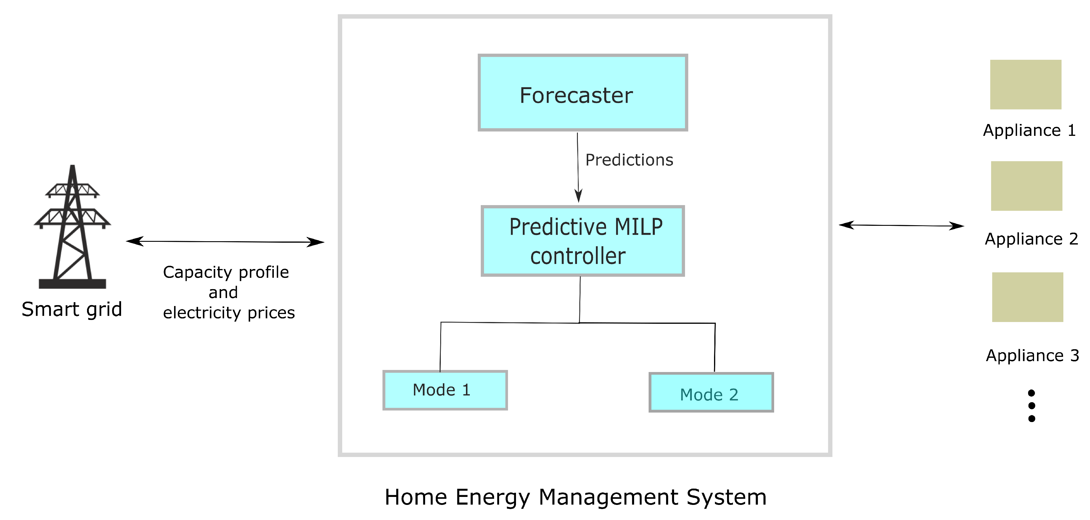
3.2. System Layout

This section provides a detailed description of the HEMS. The system architecture of the HEMS is presented in the Figure 1. The main components of the HEMS are described below.

• The first component of the HEMS is the forecaster. It is deputized to make predictions about the external weather and the heat-gains due to solar irradiance in the house. Data-driven prediction techniques [46,47] are commonly used to make these predictions based on available historical data about the variable. The second component of the HEMS uses these predictions to optimally schedule the thermal appliances.
• The second and the key component of the HEMS is the Predictive MILP controller. This component operates in two MOO, which is determined automatically within the component based upon the electrical load categories (see Section 3.1). In each mode, a different mathematical optimization problem is solved by exploiting the predictions made by the forecaster about the weather conditions. The electricity prices and the consumption-capacity profile is provided to HEMS by the smart-grid operator using smart-meter communication.

3.3. Appliance Dynamics Modeling and Setup

3.3.1. State-Space Model

In order to apply the proposed scheduling algorithm, the dynamics of all the appliances are modeled mathematically into a discrete linear time-invariant state-space representation. The discrete state-space model of a linear system with control inputs (m), outputs (p), state variables (n), and external disturbances (r) is written as in Equation (1) [48]:

$$\begin{array}{cc}\hfill & {\mathbf{x}}_{k+1}=A{\mathbf{x}}_k+B{\mathbf{u}}_k+E{\mathbf{d}}_k\hfill \\ \hfill & {\mathbf{y}}_k=C{\mathbf{x}}_k.\hfill \end{array}$$

(1)

$\mathbf{x}\in {\mathbb{R}}^n$ is the $\mathit{state\; vector}$, $\mathbf{u}\in {\mathbb{R}}^m$ is the $\mathit{control\; vector}$, $\mathbf{y}\in {\mathbb{R}}^p$ is called the $\mathit{output\; vector}$, and $\mathbf{d}\in {\mathbb{R}}^r$ is called the $\mathit{disturbance\; vector}$. Similarly, $A\in {\mathbb{R}}^{n\times n}$ is the $\mathit{state\; matrix}$, $B\in {\mathbb{R}}^{n\times m}$ is the $\mathit{control\; matrix}$, $C\in {\mathbb{R}}^{p\times n}$ is the $\mathit{output\; matrix}$, and $E\in {\mathbb{R}}^{r\times n}$ is the $\mathit{disturbance\; matrix}$. k denotes the time instant.

3.3.2. Thermal Load Appliances Modeling

For the purpose of heating the indoor environment, the house is considered to be equipped with a water source heat pump through floor heating pipes [49]. For hot water requirements, building is connected to a solar water heater system. The dynamics of both the systems is influenced by the solar irradiance and the ambient temperature.

Heat pump: A reduced order model of a residential building equipped with a heat-pump is developed in Reference [49,50] as follows using the heat balance equations:

$$\begin{array}{c}\hfill \begin{array}{cc}\hfill C_{p,r}\dot{T_r}& ={(UA)}_{fr}(T_f-T_r)-{(UA)}_{ra}(T_r-T_a)+(1-p){\varphi }_s\hfill \\ \hfill C_{p,f}\dot{T_f}& ={(UA)}_{wf}(T_w-T_f)-{(UA)}_{fr}(T_f-T_r)+p{\varphi }_s\hfill \\ \hfill C_{p,w}\dot{T_w}& =\eta W_c-{(UA)}_{wf}(T_W-T_f).\hfill \end{array}\end{array}$$

(2)

The system of Equation (2) is discretized with appropriate sample time using zero-order-hold model and written into state-space representation as in Equation (1). The first sub-equation in Equation (2) represent the thermal dynamics of the indoor environment of the building which depends upon the floor temperature $T_f$, ambient temperature $T_a$ and solar gains ${\varphi }_s$. The second sub-equation captures the heat transfer between floor and the underfloor heating system. The last sub-equation relates the temperature of the floor $T_f$ to the work done W by the compressor.

Subsequently, for heat pump state-space model, we get $\mathbf{x}={\left[\begin{array}{ccc}{T}_r& T_f& T_w\end{array}\right]}^T$, $\mathbf{u}=W_c$, $\mathbf{d}={\left[\begin{array}{cc}{T}_a& {\varphi }_s\end{array}\right]}^T$, and $\mathbf{y}=T_r$.

Solar water tank: The heat dynamics of the solar water tank is described using simple first-order differential equations as follows [51]

$$C_t\dot{T_t}={\eta }_h{P}_h+{\varphi }_s-Q_c-{(UA)}_t(T_t-T_i)$$

(3)

Equation (3) captures the thermal dynamics of the tank as a function of inlet water temperature $T_i$, power consumption of the heating element $P_h$, and solar gains ${\varphi }_s$.

After discretization and rewriting Equation (3) in state-space representation, we get $\mathbf{x}=\mathbf{y}=T_t$, $\mathbf{u}=P_h$ and $\mathbf{d}={\left[\begin{array}{ccc}{Q}_c& {\varphi }_s& T_i\end{array}\right]}^T$.

3.3.3. Non-Thermal Load Appliances Modeling

In the present work, a washing machine and a dishwasher are considered in the non-thermal load appliances category. Any non-thermal load appliance can be modeled in the same way since they have the same characteristics as described in Section 3.1.

The dynamics of a non-thermal load appliance is modeled in the following way:

$${\zeta }_{k+1}={\zeta }_k+{\psi }_k,$$

(4)

where $\zeta$ is the variable defined to keep track of the duration up to which the appliance has run, and $\psi$ is a binary integer variable which can have the values from the set {0,1}. It represents that if the appliance is running at time instant k then the value of $\psi (k)$ will be 1 and if the appliance is halted, $\psi (k)$ will be 0. In both the cases, the value of $\psi$ is added to $\zeta$. Therefore, for non-thermal appliances, Equation (4) can be represented in form of Equation (1), which subsequently gives $\mathbf{x}=\mathbf{y}=\zeta$ and $\mathbf{u}=\psi$. It should be noted that, whenever $\psi$ take the value of 1, a certain amount of power is consumed by the appliance.

4. Problem Formulation and Scheduling Algorithm

In this section, the task of the scheduling of appliances is formulated as an MILP. The appropriate constraints associated with the appliances are also described. The objective of the program is to reduce the total electricity cost and peak power consumption at the same time. As mentioned previously, an MPC framework is applied to operate the appliances. At each time step an MILP is formulated with a prediction horizon of N time steps ahead from the current time step.

4.1. Energy Cost of Thermal Appliances

The electricity cost occurred by only the energy consumption of thermal appliances is described in Equation (5) below:

$$J_{\mathcal{P}}=\sum _{k\in \mathcal{N}}\sum _{i\in \mathcal{P}}{c}_k{\mathbf{u}}_{k,i},$$

(5)

where $\mathcal{N}\in \{1,2,\cdots ,N\}$, N is the prediction horizon. $J_{\mathcal{P}}$ is the energy cost for next N time steps for running the thermal appliances. $c_k$ is the real-time electricity price at kth time step. ${\mathbf{u}}_{k,i}$ represents the power consumption by the ith thermal appliance at the time step k.

4.2. Comfort Zone Constraints of Thermal Appliances

The user would prefer to keep the temperature of the building into a prescribed comfort zone. Similarly, temperature of water in the water tank also should be in a certain temperature range according to users’ preferences. These constraints are imposed in Equation (6) as

$${\mathbf{y}}_{k,\min ,i}\le {\mathbf{y}}_{k,i}\le {\mathbf{y}}_{k,\max ,i}k\in \mathcal{N},i\in \mathcal{P},$$

(6)

where ${\mathbf{y}}_{\max ,i}$ and ${\mathbf{y}}_{\min ,i}$ are upper and lower bound on the temperature of the ith thermal appliance.

4.3. Maximum Power Consumption Constraint of Thermal Appliances

Each thermal appliance is assumed to consume up to a certain amount of power at each time step and cannot exceed that value, i.e.,

$$\begin{array}{ccc}\hfill {\mathbf{u}}_{\min ,i}\le & {\mathbf{u}}_{k,i}\le {\mathbf{u}}_{\max ,i}\hfill & \hfill k\in \mathcal{N},i\in \mathcal{P},\end{array}$$

(7)

where ${\mathbf{u}}_{\min ,i}$ and ${\mathbf{u}}_{\max ,i}$ represent the upper and lower bound on the power consumption of ith thermal appliance.

4.4. Energy Cost of Non-Thermal Appliances

Same as the thermal appliances, the electricity cost induced by the non-thermal appliances energy consumption can be considered as

$$J_{\mathcal{Q}}=\sum _{k\in \mathcal{N}}\sum _{j\in \mathcal{Q}}{c}_k{P}_{k,j}{\psi }_{k,j}\psi =\{0,1\}.$$

(8)

$J_{\mathcal{Q}}$ is the total energy cost for operating the activated non-thermal appliances. $P_{k,j}$ is the power consumed by jth non-thermal appliance at kth time step. ${\psi }_{k,j}$ is the binary variable associated to the jth non-thermal appliance at kth time step, which indicates that the appliance is ON or OFF if the value of $\psi$ is 1 or 0, respectively.

4.5. Deadline Constraint of Non-Thermal Appliances

Each non-thermal appliance run for a fixed duration as described in the Section 3.1. It has an associated deadline, by which it should finish the assigned task. This deadline is set by the user while activating the appliance and cannot be less than the running time of appliance, i.e., if user set a smaller deadline then HEMS will give a warning to reset the deadline. This can be assured by imposing the constraint in Equation (9)

$${\mathsf{\Omega }}_j\le (e_j-b_j),j\in \mathcal{Q},$$

(9)

where ${\mathsf{\Omega }}_j$ is total running time of jth appliance for which the appliance has to run in order to finish the task. $e_j$ and $b_j$ is the deadline (end time) and activation time (beginning time) of the jth appliance. It is assumed, when the appliance is turned on HEMS does not schedule it immediately rather it waits for current time slot to complete or next nearest time step to start. It should be noted that, in the present work, this constraint is not implemented in the optimization problem explicitly, rather the starting time and deadlines for non-thermal appliances are determined offline for entire simulation period as per this constraint. However, in the real-life implementation of home energy management system this constraint can be implemented directly in the optimization problem in real-time.

4.6. The Non-Thermal Appliance Start-Up Cost

In order to prevent the non-thermal appliances from being interrupted very often, there is a start-up cost associated with the each appliance, which can be represented as Equation (10)

$$J_s=\sum _{k\in \mathcal{N}}\sum _{j\in \mathcal{Q}}{\gamma }_j{\psi }_{k,j}.$$

(10)

${\gamma }_j$ refers to the start-up cost of jth non-thermal appliance.

4.7. Operation Time Constraint of Non-Thermal Appliances

To finish the task assigned, the non-thermal appliances need to run for a fixed duration $\mathsf{\Omega }$. This condition can be imposed as the following constraint:

$$\sum _{k=b_j}^{e_j}{\psi }_{k,j}={\mathsf{\Omega }}_j,j\in \mathcal{Q},\psi =\{0,1\}.$$

(11)

The constraint in Equation (11) ensures that appliance run for the its total running time between the activation time and the deadline of the appliance.

4.8. Total Capacity Constraint

This constraint put a restrain to the maximum total power consumption by all the appliances at each time step. It can be represented as following

$$\sum _{i\in \mathcal{P}}{\mathbf{u}}_{k,i}+\sum _{j\in \mathcal{Q}}{P}_{k,j}{\psi }_{k,j}\le C_{k}k\in \mathcal{N},i\in \mathcal{P},j\in \mathcal{Q},\psi \in \{0,1\}$$

(12)

$C_k$ is the total maximum power available for consumption at the time step k. The capacity constraint value is decided by the utility company. In reality, the capacity constraint value can be time varying based upon the demand of electricity and operational cost of the grid. This constraint is a hard constraint, i.e., if this constraint is not satisfied the optimization problem will halt which is not desired. To relax this constraint on total capacity, a soft constraint is introduced in next subsection.

4.9. Soft Constraints

Slack variables are introduced to allow the violation of some of the relevant constraints in Equation (13). For instance, if the desired temperature is not achieved or total power consumption exceeds the maximum available capacity, optimization routine automatically compromises between the optimal scheduling and minimization of constraint violation.

$$\begin{array}{cc}\hfill & {\mathbf{y}}_{k,\min ,i}\le {\mathbf{y}}_{k,i}+{\mathbf{v}}_{k,i}k\in \mathcal{N},i\in \mathcal{P},\hfill \end{array}$$

(13a)

$$\begin{array}{cc}\hfill & {\mathbf{y}}_{k,\max ,i}\ge {\mathbf{y}}_{k,i}-{\mathbf{v}}_{k,i}k\in \mathcal{N},i\in \mathcal{P},\hfill \end{array}$$

(13b)

$$\begin{array}{cc}\hfill & \sum _{i\in \mathcal{P}}{\mathbf{u}}_{k,i}+\sum _{j\in \mathcal{Q}}{P}_{k,j}{\psi }_{k,j}\le C_k-{\mathbf{w}}_{k}k\in \mathcal{N},i\in \mathcal{P},j\in \mathcal{Q},\hfill \end{array}$$

(13c)

where $\mathbf{v}$ and $\mathbf{w}$ are the introduced slack variable to allow violation of constraints.

4.10. Scheduling Algorithm

As the HEMS is invoked, first, it checks if any non-thermal appliance is activated from the value of activation flag (1 or 0) associated with each non-thermal appliance. If the value of activation flag is 1, then that particular non-thermal appliance is running otherwise not. Based on the value of the activation flag, the HEMS decides to operate in the following two modes:

4.10.1. Mode 1

The HEMS operates in this mode if any one or more than one non-thermal appliances are activated. In this case, the optimization problem is formulated as an MILP as follows:

$$\begin{array}{c}\hfill \begin{array}{c}\hfill \underset{\mathbf{u},\mathbf{v},\mathbf{w}}{min}{J}_{\mathcal{P}}+J_{\mathcal{Q}}+J_s+\sum _{k\in \mathcal{N}}({\beta }_{\mathbf{w}}({\mathbf{w}}_k)+\sum _{i\in \mathcal{P}}{\alpha }_{\mathbf{v},i}({\mathbf{v}}_{k,i})),\end{array}\end{array}$$

(14)

subject to

$$\begin{array}{cc}\hfill & {\mathbf{u}}_{\min ,i}\le {\mathbf{u}}_{k,i}\le {\mathbf{u}}_{\max ,i}k\in \mathcal{N},i\in \mathcal{P}\hfill \end{array}$$

(15a)

$$\begin{array}{cc}\hfill & \sum _{k=b_j}^{e_j}{\psi }_{k,j}={\mathsf{\Omega }}_j,j\in \mathcal{Q},\psi =\{0,1\}\hfill \end{array}$$

(15b)

$$\begin{array}{cc}\hfill & {\mathbf{y}}_{k,\min ,i}\le {\mathbf{y}}_{k,i}+{\mathbf{v}}_{k,i}k\in \mathcal{N},i\in \mathcal{P}\hfill \end{array}$$

(15c)

$$\begin{array}{cc}\hfill & {\mathbf{y}}_{k,\max ,i}\ge {\mathbf{y}}_{k,i}-{\mathbf{v}}_{k,i}k\in \mathcal{N},i\in \mathcal{P}\hfill \end{array}$$

(15d)

$$\begin{array}{cc}\hfill & \sum _{i\in \mathcal{P}}{\mathbf{u}}_{k,i}+\sum _{j\in \mathcal{Q}}{P}_{k,j}{\psi }_{k,j}\le C_k-{\mathbf{w}}_{k}k\in \mathcal{N},i\in \mathcal{P},j\in \mathcal{Q}.\hfill \end{array}$$

(15e)

Here, ${\alpha }_{\mathbf{v}}(\mathbf{v})\ge 0$ and ${\beta }_{\mathbf{w}}(\mathbf{w})\ge 0$ are convex penalty cost functions associated with the slack variables $\mathbf{v}$ and $\mathbf{w}$. It should be noted that the value of ${\beta }_{\mathbf{w}}(\mathbf{w})$ is time dependent and is specified by the power utility depending upon the power-grid operation and stability. This information is shared with HEMS dynamically on a real-time basis.

4.10.2. Mode 2

In Mode 2, since only the thermal appliances are running, the optimization problem is formulated just as a linear program (LP) rather than MILP

$$min{J}_{\mathcal{P}},$$

(16)

subject to

$$\begin{array}{cc}\hfill & {\mathbf{u}}_{\min ,i}\le {\mathbf{u}}_{k,i}\le {\mathbf{u}}_{\max ,i}k\in \mathcal{N},i\in \mathcal{P},\hfill \end{array}$$

(17a)

$$\begin{array}{cc}\hfill & {\mathbf{y}}_{k,\min ,i}\le {\mathbf{y}}_{k,i}+{\mathbf{v}}_{k,i}k\in \mathcal{N},i\in \mathcal{P},\hfill \end{array}$$

(17b)

$$\begin{array}{cc}\hfill & {\mathbf{y}}_{k,\max ,i}\ge {\mathbf{y}}_{k,i}-{\mathbf{v}}_{k,i}k\in \mathcal{N},i\in \mathcal{P},\hfill \end{array}$$

(17c)

$$\begin{array}{cc}\hfill & \sum _{i\in \mathcal{P}}{\mathbf{u}}_{k,i}\le C_k-{\mathbf{w}}_{k}k\in \mathcal{N},i\in \mathcal{P}.\hfill \end{array}$$

(17d)

The above constraint considers the total power consumption by only the thermal appliances, since no non-thermal appliance is running.

In both the modes, at each time step, a control decision policy ${\left\{{\mathbf{u}}_k^{*}\right\}}_{k=1}^N$ is obtained for next N time steps by solving the formulated optimization. MILP and only the first control input $\left\{{\mathbf{u}}_1^{*}\right\}$ is applied to the system and rest of the control inputs ${\left\{{\mathbf{u}}_k^{*}\right\}}_{k=2}^N$ are discarded. The optimization problem is formulated and solved again in the similar manner at the next time step as per the receding horizon strategy.

For the present study, it is assumed that perfect electricity prices forecast and weather forecast are available as this is not the focus of the paper.

5. Simulation Studies

5.1. Simulation Setup

As mentioned previously, we consider heat pump and solar water heater as thermal appliances for current simulation studies.

Table 1. Thermal appliance parameters.

Parameter	Value	Unit	Parameter	Value	Unit
$C_{p,f}$	3315	kJ/${}^{°}$C	${(UA)}_{fr}$	624	kJ/${}^{°}$Ch
$C_{p,r}$	810	kJ/${}^{°}$C	${(UA)}_{wf}$	28	kJ/${}^{°}$Ch
$C_{p,w}$	836	kJ/${}^{°}$C	${(UA)}_{wf}$	28	kJ/${}^{°}$Ch
$C_t$	3881.3	kJ/${}^{°}$C	${(UA)}_t$	29.84	kJ/${}^{°}$Ch
$\eta$	3	-	p	0.2	-
${\eta }_h$	1	-

contains the values of the parameters used in modeling of thermal appliances as described in Reference [49,51]. To put a constraint on the indoor air temperature, (18 ${}^{°}$C, 22 ${}^{°}$C) is specified as the desired comfort range. These constraints can be chosen to be time varying also. The heat pump is considered to consume maximum of 1 kW power at each time step. Similarly, the water temperature in. the solar water heater tank is kept bounded between (50 ${}^{°}$C, 70 ${}^{°}$C) and the maximum power consumption of the water heater is considered to be 2 kW. Everyday water withdrawal demand profile is obtained from the DHWcalc toolbox [52], which generates realistic domestic hot water demand depending upon various characteristics like number of households, total mean daily draw off volume, etc.

Without any loss of generality, a washing machine and dishwasher are considered as the non-thermal household appliances.

Table 2. Non-thermal appliance parameters.

Appliance	Running Time ($\mathsf{\Omega }$)	Rated-Power (P)
Washing machine	2 h	3 kW
Dishwasher	2.5 h	4 kW

details the parameter values for the washing machine and the dishwasher. Every day, non-thermal appliance requests are activated at random time steps with a random deadline which is greater than the total running time of the appliance.

The entire simulation setup is implemented in MATLAB. For simulation purpose, ambient temperature $T_a$ and solar radiation ${\varphi }_s$ are obtained from ASHRAE IWEC (International Weather for Energy Calculations) weather data files for Dublin, Ireland [53]. The electricity prices are taken from wholesale Danish Energy Market data [54] and employed for real time implementation of the proposed algorithm. A maximum capacity constraint of 4 kW is imposed on the total power consumption of all the appliances. In reality, the capacity constraints can be time varying. The setup is simulated over a 7-day period with a prediction horizon of 24 h (Mode 1). To solve the MILP, Gurobi solver is used in integration with YALMIP toolbox [55] and MATLAB. To summarize,

Table 3. Optimization problem parameters.

Mode	Number of Constraints	Optimization Problem
Mode 1 (washing machine)	7003	Mixed Integer Linear Program
Mode 1 (dryer)	7003	Mixed Integer Linear Program
Mode 1 (washing machine and dryer)	7290	Mixed Integer Linear Program
Mode 2	6716	Linear program

shows the number of constraints and optimization methods associated with each mode.

5.2. Results and Discussion

Figure 2 depicts the variation of the indoor air temperature and the power consumed by the heat pump to maintain that temperature. During the entire simulation, the indoor temperature stays within the subjected comfort zone boundaries and the constraint on the power consumption of the heat pump is also satisfied.

Similarly, Figure 3 presents the temperature variation of water in the water tank, and the power consumed by the water heater, respectively. The initial water temperature is considered to be at 20 ${}^{°}$C (see Figure 3a). As the time passes, the temperature gradually increases over next few hours and then it is maintained inside the specified temperature range. This also explains the fact that the power consumed by the water heater is high in beginning of the simulation period in Figure 3b.

Figure 4a,b shows the power consumed by the washing machine and the dishwasher, respectively. It can be seen that the appliances operation is interrupted occasionally in order to minimize the electricity cost and satisfy the capacity constraints. It should be noted that, the HEMS has no knowledge about the arrival request of washing-machine and dishwasher. The arrival requests are generated randomly to investigate the capability of the HEMS to handle immediate request situations.

In order to assess the performance of the proposed method, the following different scenarios were simulated.

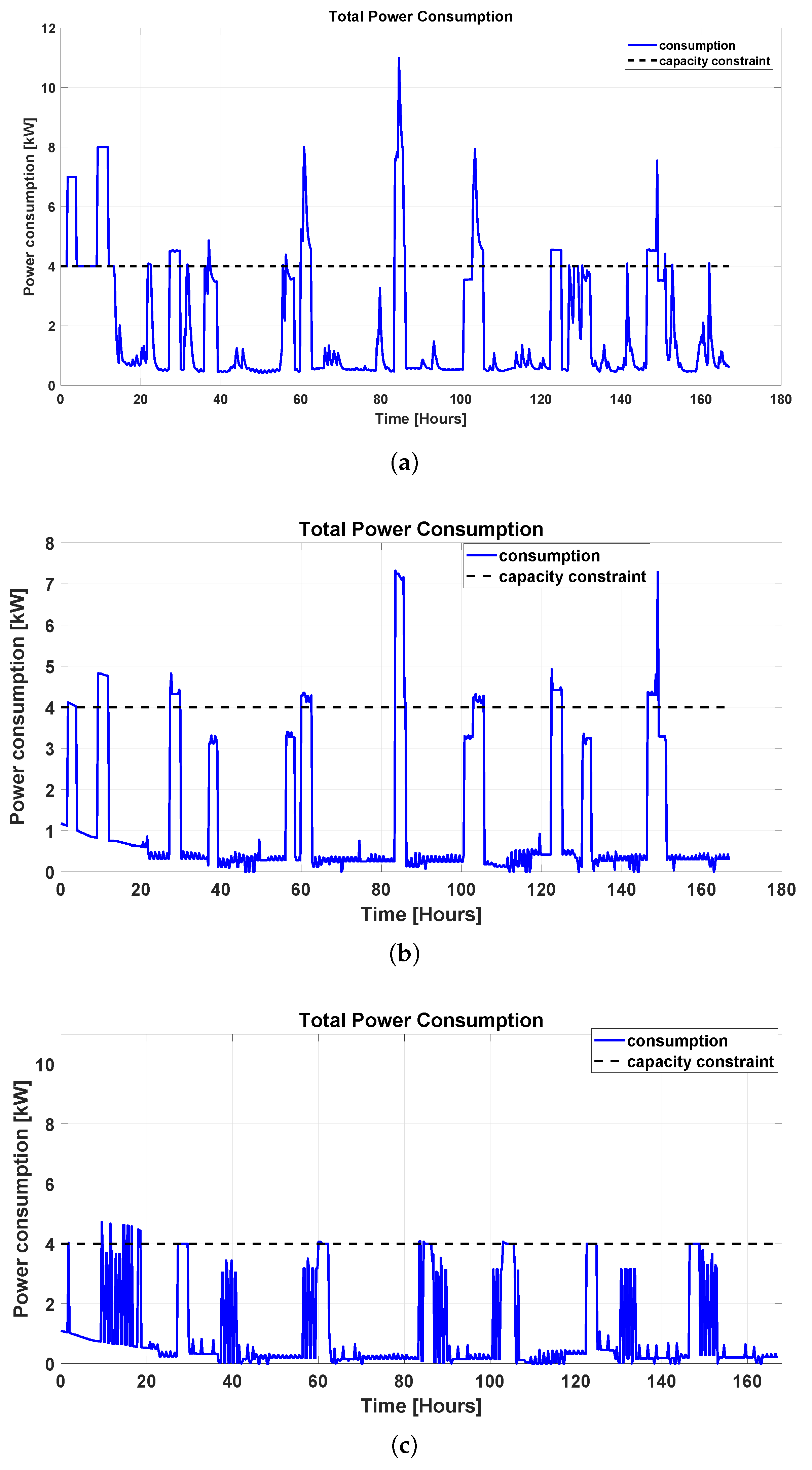
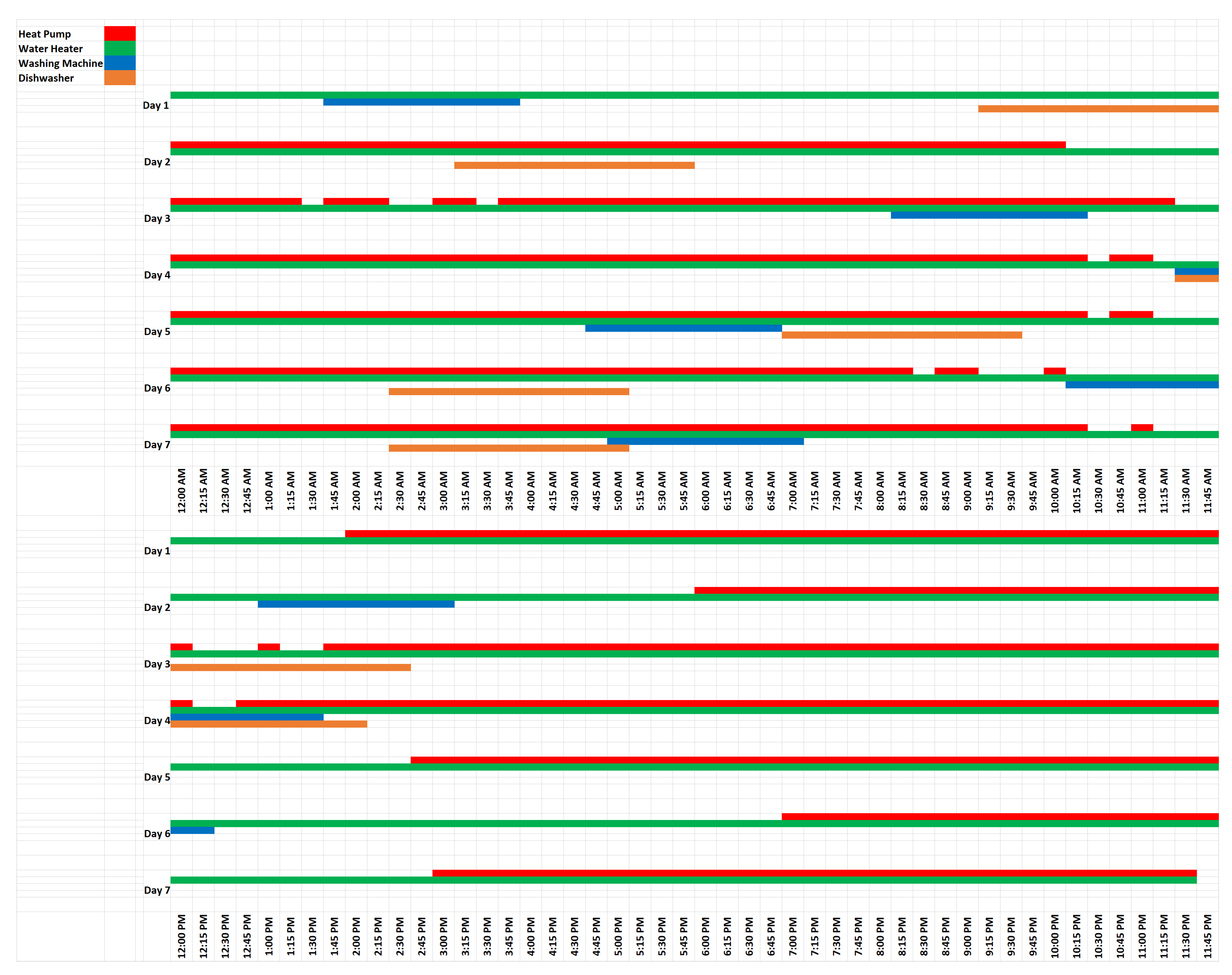
5.2.1. Without HEMS and Linear Quadratic Regulation (LQR) Control for Thermal Appliances

In this case, it was considered that there is no HEMS to schedule the appliances, however, the thermal appliances were operated using LQR feedback control. This control strategy is a state-feedback control method in which the control input u is given by the feedback control law: $u=-Kx$, where x is the state of the system and K is the control gain which is obtained by solving Riccati differential equation.

Figure 5a shows the total power consumption of all the appliances in this case. It can be seen in the figure that initially the power consumption violates the capacity constraints because the water heater runs at full power due to the low initial temperature of water. The maximum power consumption is at 11 kW. The operation schedule of appliances in this case is given in Figure 6. In this case, thermal appliances are almost always running, since the controller tries to track the set point at each time step. However, this could be changed by providing time-varying constraints on the set points. Clearly, we see that the non-thermal appliances are never interrupted and run continuously once started. In Figure 6, on the noon of the fourth day of the week, the water heater, washing machine, and dishwasher are operating all together at their respective maximum rated-power, which brings the total power consumption to 11 kW.

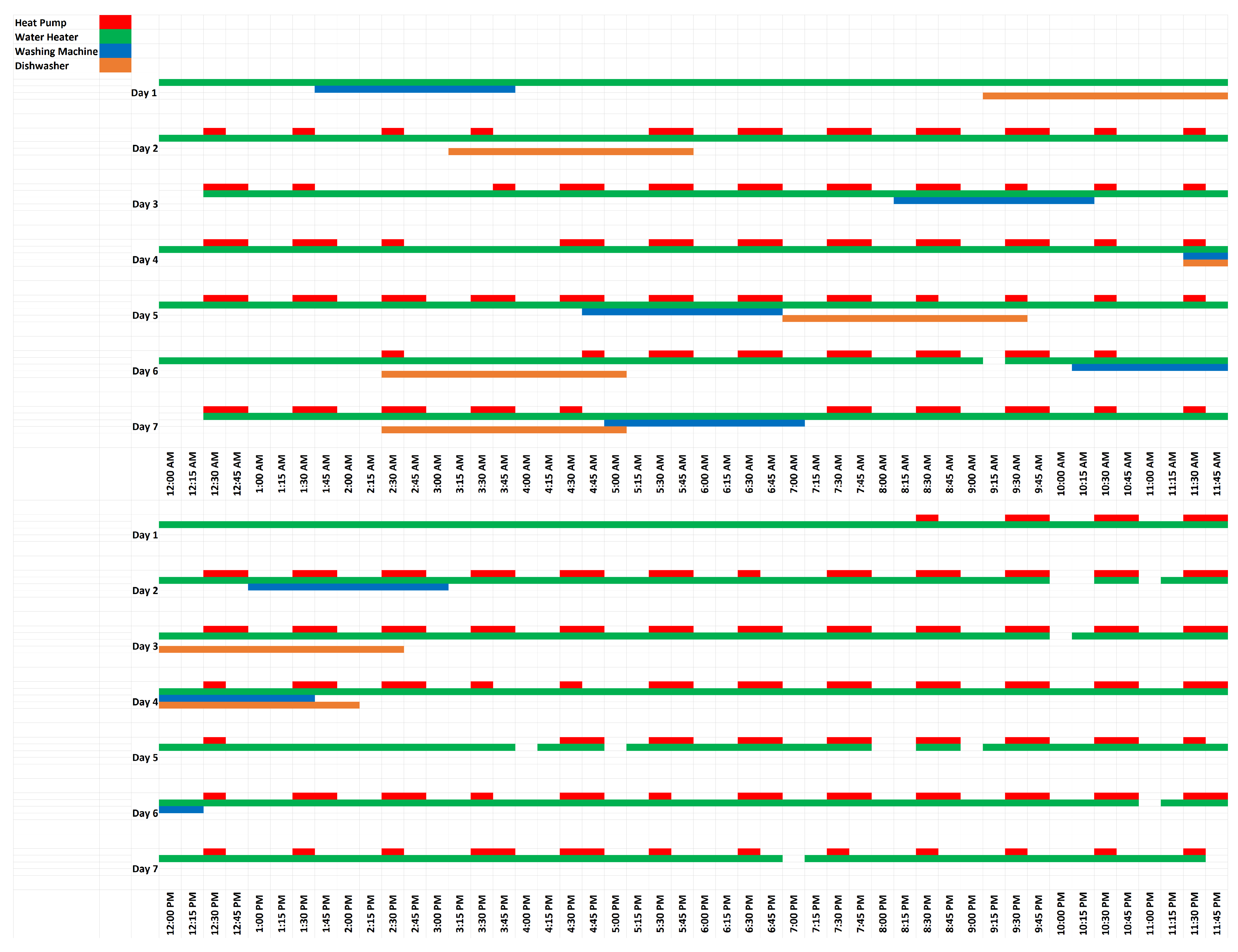
5.2.2. Without HEMS and MPC Control for Thermal Appliances

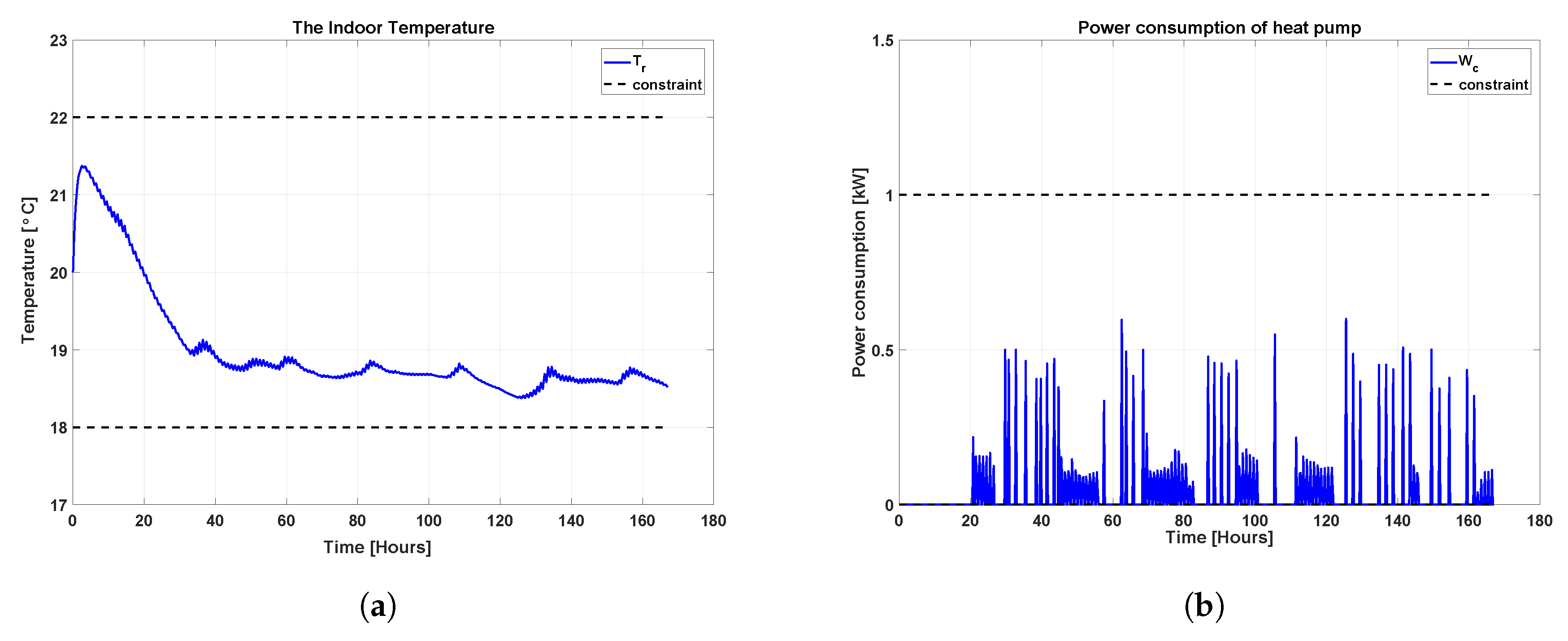
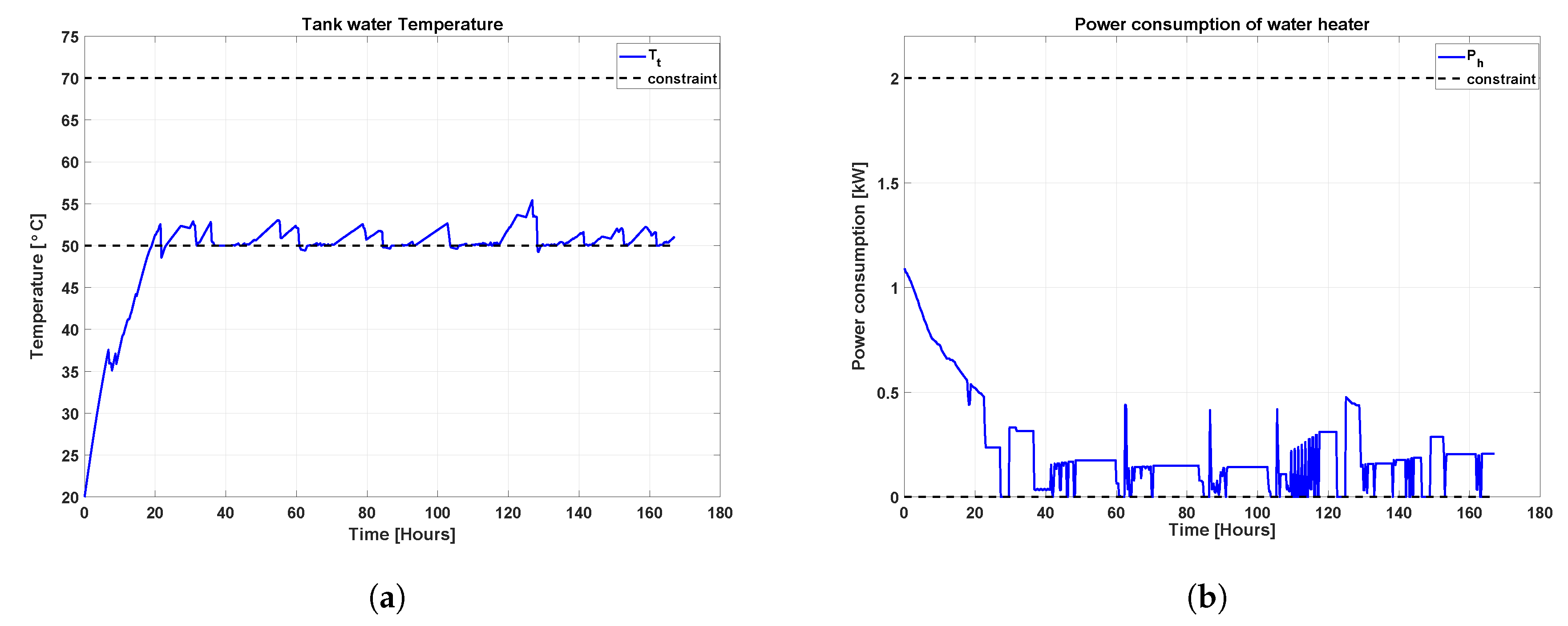
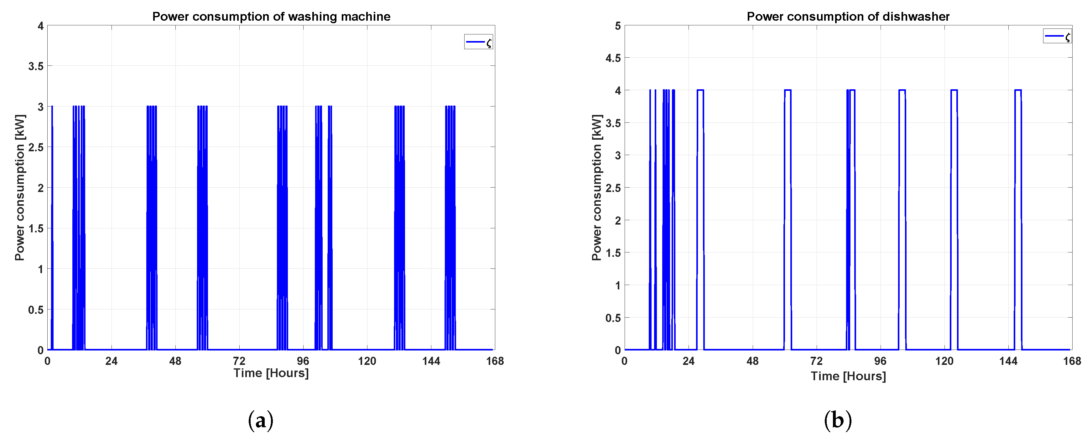
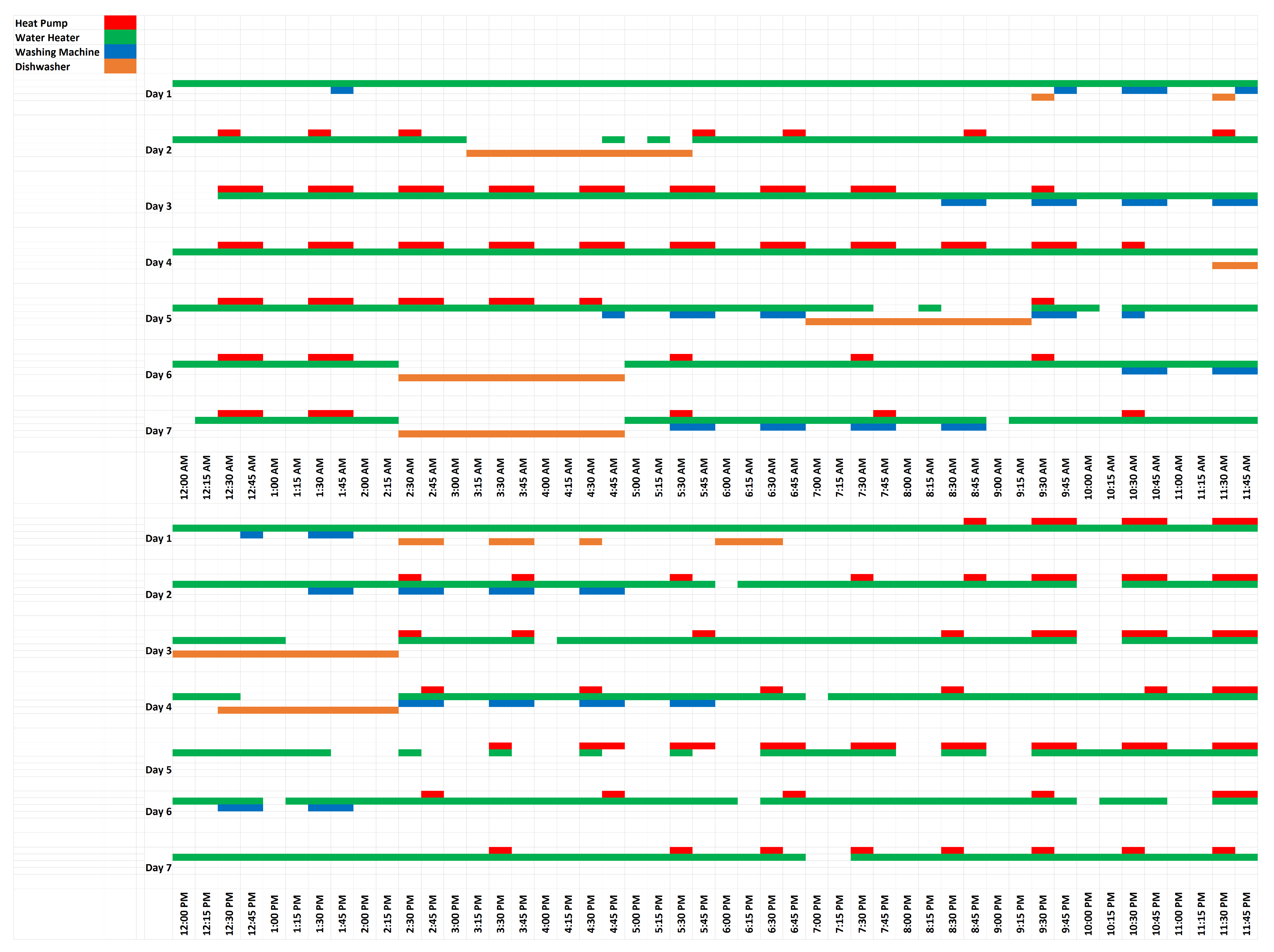
In this case, there also is no HEMS to schedule the appliances in this case also. But the thermal appliances are operated using MPC strategy, which is an advanced control technique in comparison to LQR control. Figure 5b shows the total power consumption in this case. It was observed that the peak power consumption in this case is reduced to around 7.5 kW which occurs at around 12:30 PM on the fourth day. It can seen in the Figure 7 that all the appliances (thermal and non-thermal appliances) are in operation at this time which implies that only 0.5 kW power is consumed by the thermal appliances. This happen because the MPC has prior knowledge of the external disturbances (MPC), so it operates the appliances to comply with the subjected constraint of maximum peak-power consumption. Clearly, using MPC instead of LQR controller is useful to reduce the peak-power consumption.

5.2.3. With HEMS

In this scenario, there is HEMS employed in the house to schedule the appliances. All the appliances are scheduled using MPC strategy in this case. Figure 5c clearly depicts the benefits of using HEMS and presents the total power consumed by all the household appliances. In Figure 5c, it can be seen that for initial time steps, total power consumption goes beyond the capacity limit of 4 kW, which happens due to the high power consumption of water heater since initial water temperature in the tank is low. At later time steps, it can be seen that the maximum total power consumed by all the appliances stays around the capacity limit. The constraints on the capacity limit are allowed to violate to ensure the feasibility of the optimization problem (soft constraints).

Figure 8 shows the operation schedule of the appliances in this case. It can be seen that, the non-thermal appliances are interrupted occasionally to satisfy the capacity constraints and minimize the electricity cost. For example, at the noon of the fourth day of the week, washing-machine and the dishwasher is not running rather they are shifted to run later in the day.

The total electricity cost as per the time varying prices used in this study, is detailed in the

Table 4. The total electricity cost for the entire simulation duration.

Case	Electricity Cost (€)
Without HEMS and LQR control	15.14
Without HEMS and MPC control	8.2005
With HEMS	4.4934

. It should be noted that this includes the cost of running both thermal and non-thermal appliances for entire simulation period. In comparison to the case without HEMS and LQR controller for the thermal appliances, a reduction of 70% is achieved in total electricity cost by using the HEMS. Similarly, in comparison to the case without HEMS and MPC controller for the thermal appliances, the HEMS achieves a reduction of 45%.

To see the effectiveness of HEMS in reducing the peak-load, the total violation of the capacity constraint over the simulation period and the maximum peak-load consumed by the appliances for all the cases was calculated, and is presented in

Table 5. Total violation of capacity constraint during the simulation period.

Case	Overconsumption (kW)	Peak-Power Consumption (kW)
Without HEMS and LQR control	172	12.98
Without HEMS and MPC control	59.8947	7.3
With HEMS	6.4062	4.7285

. The total violation for the case when appliances are scheduled with HEMS is about 10 times lower than the case of no HEMS with MPC control for thermal appliances. Similarly, by using HEMS, the peak power consumption is reduced by 57% and 35% in comparison with the case of no HEMS with LQR control and MPC control for thermal appliances, respectively. The PAR for all the cases is detailed in the

Table 6. Peak to average ratio.

Case	Peak-Power Consumption (kW)	Mean-Power Consumption (kW)	PAR
Without HEMS and LQR control	11	1.88	5.82
Without HEMS and MPC control	7.31	1.10	6.65
With HEMS	4.7285	0.937	5.04

. It is observed that by using the HEMS, PAR is reduced by 35% and 24% in comparison to other two cases.

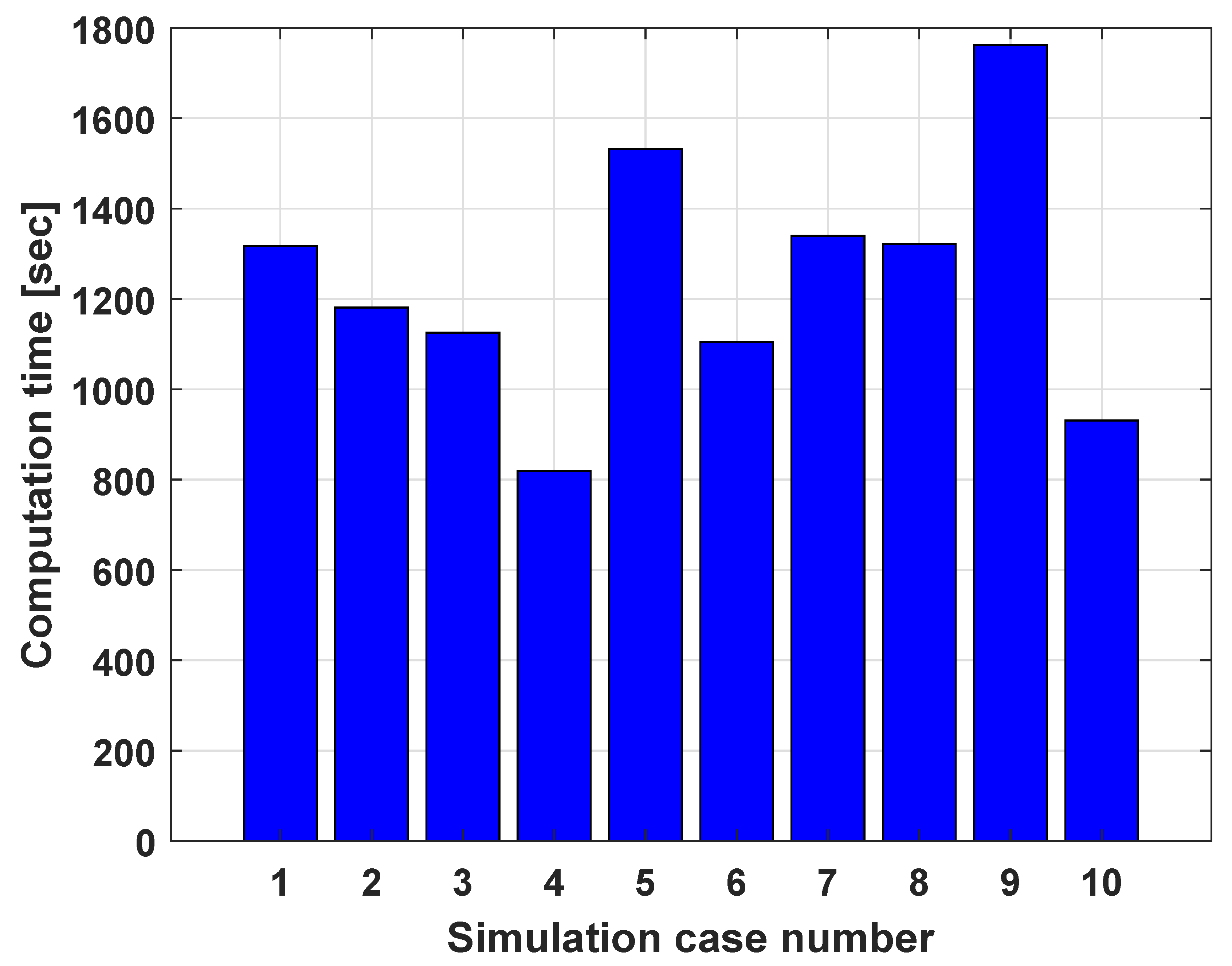
5.3. Computation Time of HEMS

The simulations were carried out in MATLAB on a computer with Intel(R) Core(TM) i7-5600 CPU with 16 GB RAM. Since, the non-thermal appliances can start at any time of the day, 10 different simulation with random starting time of non-thermal appliances are run. The computation time for each case is recorded and presented in Figure 9. The average computation time for each case came out to be 1243.6 s, i.e., 1.8 s per time step.

6. Conclusions

In this work, the problem of scheduling of appliances to achieve reduction in the peak-load and total electricity cost has been investigated using model predictive control (MPC). An architecture of a home energy management system (HEMS) was presented which operate in two modes of operations (MOOs) based upon the categorization of the appliances (thermal and non-thermal). The system dynamics of the appliances was modeled into a state-space formulation.

The proposed approach was able to schedule the appliances dynamically as the optimization problem is formulated and solved at each time step. The proposed framework was shown to provide flexibility to the user to turn the non-thermal appliances at any time step while achieving the objective of cost minimization. The simulation results showed the reductions of up to 70% in the total electricity cost and up to 57% in the peak power consumption, as well. The operation schedule of appliances with and without HEMS was also compared. The non-thermal appliances were able to interrupt and shift the operation to the low electricity price periods while finishing the task by the deadline.

The future work will include the consideration of energy storage facility (thermal and electric) [56,57], renewable energy generation, and integration of plug-in electric vehicle (PEVs) into the framework. In addition, the framework will be scaled up to a small community or a group of houses to investigate the demand-response from the perspective of power utility or aggregator companies.

References

1. Pérez-Lombard, L.; Ortiz, J.; Pout, C. A review on buildings energy consumption information. Energy Build. 2008, 40, 394–398. [Google Scholar] [CrossRef]
2. Andersen, P.B.; Hauksson, E.B.; Pedersen, A.B.; Gantenbein, D.; Jansen, B.; Andersen, C.A.; Dall, J. Smart Grid Applications, Communications, and Security; Wiley-VCH: Weinheim, Germany, 2012. [Google Scholar]
3. Strbac, G. Demand side management: Benefits and challenges. Energy Policy 2008, 36, 4419–4426. [Google Scholar] [CrossRef]
4. Albadi, M.H.; El-Saadany, E. Demand response in electricity markets: An overview. In Proceedings of the 2007 IEEE Power Engineering Society General Meeting, Tampa, FL, USA, 24–28 June 2007. [Google Scholar]
5. Palensky, P.; Dietrich, D. Demand side management: Demand response, intelligent energy systems, and smart loads. IEEE Trans. Ind. Inform. 2011, 7, 381–388. [Google Scholar] [CrossRef] [Green Version]
6. Brambley, M.R.; Hansen, D.; Haves, P.; Holmberg, D.; McDonald, S.; Roth, K.; Torcellini, P. Advanced sensors and controls for building applications: Market assessment and potential R&D pathways. Pac. Northwest Natl. Lab. 2005. [Google Scholar] [CrossRef] [Green Version]
7. Stankovic, J.A. Real-Time Computing System: The Next Generation; University of Massachusetts: Amherst, MA, USA, 1988. [Google Scholar]
8. De Angelis, F.; Boaro, M.; Fuselli, D.; Squartini, S.; Piazza, F.; Wei, Q. Optimal home energy management under dynamic electrical and thermal constraints. IEEE Trans. Ind. Inform. 2013, 9, 1518–1527. [Google Scholar] [CrossRef]
9. Adika, C.O.; Wang, L. Autonomous appliance scheduling for household energy management. IEEE Trans. Smart Grid 2014, 5, 673–682. [Google Scholar] [CrossRef]
10. Mohsenian-Rad, A.H.; Leon-Garcia, A. Optimal residential load control with price prediction in real-time electricity pricing environments. IEEE Trans. Smart Grid 2010, 1, 120–133. [Google Scholar] [CrossRef]
11. Setlhaolo, D.; Xia, X. Optimal scheduling of household appliances with a battery storage system and coordination. Energy Build. 2015, 94, 61–70. [Google Scholar] [CrossRef]
12. Paterakis, N.G.; Erdinc, O.; Bakirtzis, A.G.; Catalão, J.P. Optimal household appliances scheduling under day-ahead pricing and load-shaping demand response strategies. IEEE Trans. Ind. Inform. 2015, 11, 1509–1519. [Google Scholar] [CrossRef]
13. Shirazi, E.; Jadid, S. Optimal residential appliance scheduling under dynamic pricing scheme via HEMDAS. Energy Build. 2015, 93, 40–49. [Google Scholar] [CrossRef]
14. Sou, K.C.; Weimer, J.; Sandberg, H.; Johansson, K.H. Scheduling smart home appliances using mixed integer linear programming. In Proceedings of the 2011 50th IEEE Conference on Decision and Control and European Control Conference, Orlando, FL, USA, 12–15 December 2011; pp. 5144–5149. [Google Scholar]
15. Shirazi, E.; Zakariazadeh, A.; Jadid, S. Optimal joint scheduling of electrical and thermal appliances in a smart home environment. Energy Convers. Manag. 2015, 106, 181–193. [Google Scholar] [CrossRef]
16. Paridari, K.; Parisio, A.; Sandberg, H.; Johansson, K.H. Robust Scheduling of Smart Appliances in Active Apartments With User Behavior Uncertainty. IEEE Trans. Autom. Sci. Eng. 2016, 13, 247–259. [Google Scholar] [CrossRef]
17. Wu, X.; Hu, X.; Yin, X.; Moura, S. Stochastic optimal energy management of smart home with PEV energy storage. IEEE Trans. Smart Grid 2016, 9, 2065–2075. [Google Scholar] [CrossRef]
18. Matallanas, E.; Castillo-Cagigal, M.; Gutiérrez, A.; Monasterio-Huelin, F.; Caamaño-Martín, E.; Masa, D.; Jiménez-Leube, J. Neural network controller for active demand-side management with PV energy in the residential sector. Appl. Energy 2012, 91, 90–97. [Google Scholar] [CrossRef] [Green Version]
19. Soares, A.; Antunes, C.H.; Oliveira, C.; Gomes, Á. A multi-objective genetic approach to domestic load scheduling in an energy management system. Energy 2014, 77, 144–152. [Google Scholar] [CrossRef]
20. Graditi, G.; Di Silvestre, M.L.; Gallea, R.; Sanseverino, E.R. Heuristic-based shiftable loads optimal management in smart micro-grids. IEEE Trans. Ind. Inform. 2015, 11, 271–280. [Google Scholar] [CrossRef]
21. Logenthiran, T.; Srinivasan, D.; Shun, T.Z. Demand side management in smart grid using heuristic optimization. IEEE Trans. Smart Grid 2012, 3, 1244–1252. [Google Scholar] [CrossRef]
22. Aslam, S.; Iqbal, Z.; Javaid, N.; Khan, Z.; Aurangzeb, K.; Haider, S. Towards efficient energy management of smart buildings exploiting heuristic optimization with real time and critical peak pricing schemes. Energies 2017, 10, 2065. [Google Scholar] [CrossRef] [Green Version]
23. Gutierrez-Martinez, V.J.; Moreno-Bautista, C.A.; Lozano-Garcia, J.M.; Pizano-Martinez, A.; Zamora-Cardentas, E.A.; Gomez-Martinez, M.A. A Heuristic Home Electric Energy Management System Considering Renewable Energy Availability. Energies 2019, 12, 671. [Google Scholar] [CrossRef] [Green Version]
24. Meng, F.L.; Zeng, X.J. A bilevel optimization approach to demand response management for the smart grid. In Proceedings of the 2016 IEEE Congress on Evolutionary Computation (CEC), Vancouver, BC, Canada, 24–29 July 2016; pp. 287–294. [Google Scholar]
25. Chen, C.; Kishore, S.; Snyder, L.V. An innovative RTP-based residential power scheduling scheme for smart grids. In Proceedings of the 2011 IEEE International Conference on Acoustics, Speech and Signal Processing (ICASSP), Prague, Czech Republic, 22–27 May 2011; pp. 5956–5959. [Google Scholar]
26. Zhang, D.; Li, S.; Sun, M.; O’Neill, Z. An optimal and learning-based demand response and home energy management system. IEEE Trans. Smart Grid 2016, 7, 1790–1801. [Google Scholar] [CrossRef]
27. Ozturk, Y.; Senthilkumar, D.; Kumar, S.; Lee, G.K. An Intelligent Home Energy Management System to Improve Demand Response. IEEE Trans. Smart Grid 2013, 4, 694–701. [Google Scholar] [CrossRef]
28. Setlhaolo, D.; Xia, X.; Zhang, J. Optimal scheduling of household appliances for demand response. Electr. Power Syst. Res. 2014, 116, 24–28. [Google Scholar] [CrossRef]
29. Haider, H.T.; See, O.H.; Elmenreich, W. Dynamic residential load scheduling based on adaptive consumption level pricing scheme. Electr. Power Syst. Res. 2016, 133, 27–35. [Google Scholar] [CrossRef]
30. Pipattanasomporn, M.; Kuzlu, M.; Rahman, S. An algorithm for intelligent home energy management and demand response analysis. IEEE Trans. Smart Grid 2012, 3, 2166–2173. [Google Scholar] [CrossRef]
31. Costanzo, G.T.; Zhu, G.; Anjos, M.F.; Savard, G. A system architecture for autonomous demand side load management in smart buildings. IEEE Trans. Smart Grid 2012, 3, 2157–2165. [Google Scholar] [CrossRef]
32. Rastegar, M.; Fotuhi-Firuzabad, M.; Zareipour, H. Home energy management incorporating operational priority of appliances. Int. J. Electr. Power Energy Syst. 2016, 74, 286–292. [Google Scholar] [CrossRef]
33. Garcia, C.E.; Prett, D.M.; Morari, M. Model predictive control: Theory and practice—A survey. Automatica 1989, 25, 335–348. [Google Scholar] [CrossRef]
34. Ma, J.; Qin, J.; Salsbury, T.; Xu, P. Demand reduction in building energy systems based on economic model predictive control. Chem. Eng. Sci. 2012, 67, 92–100. [Google Scholar] [CrossRef]
35. Oldewurtel, F.; Ulbig, A.; Parisio, A.; Andersson, G.; Morari, M. Reducing peak electricity demand in building climate control using real-time pricing and model predictive control. In Proceedings of the 49th IEEE Conference on Decision and Control (CDC), Atlanta, GA, USA, 15–17 December 2010; pp. 1927–1932. [Google Scholar]
36. Bianchini, G.; Casini, M.; Vicino, A.; Zarrilli, D. Demand-response in building heating systems: A Model Predictive Control approach. Appl. Energy 2016, 168, 159–170. [Google Scholar] [CrossRef]
37. Li, K.; Wenping, X.; Xu, C.; Mao, H. A multiple model approach for predictive control of indoor thermal environment with high resolution. J. Build. Perform. Simul. 2018, 11, 164–178. [Google Scholar] [CrossRef]
38. Corbin, C.; Henze, G. Predictive control of residential HVAC and its impact on the grid. Part II: Simulation studies of residential HVAC as a supply following resource. J. Build. Perform. Simul. 2017, 10, 365–377. [Google Scholar] [CrossRef]
39. Pedersen, T.H.; Petersen, S. Investigating the performance of scenario-based model predictive control of space heating in residential buildings. J. Build. Perform. Simul. 2018, 11, 485–498. [Google Scholar] [CrossRef]
40. Zhang, Y.; Zhang, T.; Wang, R.; Liu, Y.; Guo, B. Optimal operation of a smart residential microgrid based on model predictive control by considering uncertainties and storage impacts. Sol. Energy 2015, 122, 1052–1065. [Google Scholar] [CrossRef]
41. Zhang, Y.; Wang, R.; Zhang, T.; Liu, Y.; Guo, B. Model predictive control-based operation management for a residential microgrid with considering forecast uncertainties and demand response strategies. IET Gener. Transm. Distrib. 2016, 10, 2367–2378. [Google Scholar] [CrossRef]
42. Parisio, A.; Rikos, E.; Tzamalis, G.; Glielmo, L. Use of model predictive control for experimental microgrid optimization. Appl. Energy 2014, 115, 37–46. [Google Scholar] [CrossRef]
43. Pascual, J.; Barricarte, J.; Sanchis, P.; Marroyo, L. Energy management strategy for a renewable-based residential microgrid with generation and demand forecasting. Appl. Energy 2015, 158, 12–25. [Google Scholar] [CrossRef]
44. Chen, C.; Wang, J.; Heo, Y.; Kishore, S. MPC-based appliance scheduling for residential building energy management controller. IEEE Trans. Smart Grid 2013, 4, 1401–1410. [Google Scholar] [CrossRef]
45. Rahmani-Andebili, M. Scheduling deferrable appliances and energy resources of a smart home applying multi-time scale stochastic model predictive control. Sustain. Cities Soc. 2017, 32, 338–347. [Google Scholar] [CrossRef]
46. Hammer, A.; Heinemann, D.; Lorenz, E.; Lückehe, B. Short-term forecasting of solar radiation: A statistical approach using satellite data. Sol. Energy 1999, 67, 139–150. [Google Scholar] [CrossRef]
47. Mellit, A.; Pavan, A.M. A 24-h forecast of solar irradiance using artificial neural network: Application for performance prediction of a grid-connected PV plant at Trieste, Italy. Sol. Energy 2010, 84, 807–821. [Google Scholar] [CrossRef]
48. Brogan, W.L. Modern Control Theory; Pearson Education India: New Delhi, India, 1982. [Google Scholar]
49. Halvgaard, R.; Poulsen, N.K.; Madsen, H.; Jørgensen, J.B. Economic model predictive control for building climate control in a smart grid. In Proceedings of the 2012 IEEE PES Innovative Smart Grid Technologies (ISGT), Washington, DC, USA, 16–20 January 2012; pp. 1–6. [Google Scholar]
50. Staino, A.; Nagpal, H.; Basu, B. Cooperative optimization of building energy systems in an economic model predictive control framework. Energy Build. 2016, 128, 713–722. [Google Scholar] [CrossRef] [Green Version]
51. Halvgaard, R.; Bacher, P.; Perers, B.; Andersen, E.; Furbo, S.; Jørgensen, J.B.; Poulsen, N.K.; Madsen, H. Model predictive control for a smart solar tank based on weather and consumption forecasts. Energy Procedia 2012, 30, 270–278. [Google Scholar] [CrossRef] [Green Version]
52. Jordan, U.; Vajen, K. DHWcalc: Program to generate domestic hot water profiles with statistical means for user defined conditions. In Proceedings of the ISES Solar World Congress, Orlando, FL, USA, 8–12 August 2005; pp. 8–12. [Google Scholar]
53. Energy Plus Energy Simulation Software-International Weather for Energy. Calculations (IWEC) Data for Ireland. Available online: http://apps1.eere.energy.gov/buildings/energyplus/cfm/weather_data3.cfm/region=6_europe_wmo_region_6/country=IRL/cname=Ireland (accessed on 30 December 2019).
54. Danish Electricity Wholesale Market. Available online: http://www.energinet.dk/EN/El/Engrosmarked/Sider/default.aspx (accessed on 20 June 2018).
55. Löfberg, J. YALMIP: A Toolbox for Modeling and Optimization in MATLAB. In Proceedings of the 2004 IEEE International Conference on Robotics and Automation (IEEE Cat. No.04CH37508), New Orleans, LA, USA, 2–4 September 2004. [Google Scholar]
56. Vatu, R.; Seritan, G.; Ceaki, O.; Mancasi, M. Microgrids operation improvement using storage technologies. In Proceedings of the 2017 10th International Symposium on Advanced Topics in Electrical Engineering (ATEE), Bucharest, Romania, 23–25 March 2017; pp. 791–796. [Google Scholar]
57. Enescu, D.; Chicco, G.; Porumb, R.; Seritan, G. Thermal Energy Storage for Grid Applications: Current Status and Emerging Trends. Energies 2020, 13, 340. [Google Scholar] [CrossRef] [Green Version]
Figure 1. System architecture of HEMS. MILP = mixed-integer-linear-programming.
Applsci 10 01627 g001
Figure 2. (a) Room temperature with HEMS; (b) power consumption by heat pump with HEMS.
Applsci 10 01627 g002
Figure 3. (a) Temperature of water in water tank with HEMS; (b) power consumption by solar water heater with HEMS.
Applsci 10 01627 g003
Figure 4. (a) Power consumption of washing machine with HEMS; (b) power consumption of dishwasher with HEMS.
Applsci 10 01627 g004
Figure 5. (a) Total power consumption of the appliances without HEMS and Linear Quadratic Regulation (LQR) control for the thermal appliances; (b) total power consumption of the appliances without HEMS and model predictive control (MPC) for the thermal appliances; (c) total power consumption of the appliances with HEMS.
Applsci 10 01627 g005
Figure 6. The operation schedule of the appliances without HEMS and LQR control for the thermal appliances.
Applsci 10 01627 g006
Figure 7. The operation schedule of the appliances without HEMS and. MPC control for the thermal appliances.
Applsci 10 01627 g007
Figure 8. Operation schedule of the appliances with HEMS.
Applsci 10 01627 g008
Figure 9. The computation time for the simulation period for 10 simulation cases.
Applsci 10 01627 g009