RUL Prediction of Railway PCCS Based on Wiener Process Model with Unequal Interval Wear Data

Abstract

The railway pantograph carbon contact strip (PCCS) plays a critical role in collecting the electric current from the catenary to guarantee the steady power supply for the train. The catenary contacts with the PCCS and slides from one side to another side when the train runs on the track, which generates the wear on the surface of the PCCS. The thickness of the PCCS cannot be smaller than a lower limit for the sake of safety. Therefore, the remaining useful life (RUL) prediction of the PCCS is beneficial for the pantograph maintenance and inventory management. In this paper, the wear data from Guangzhou Metro are analyzed in the first place. After that, the challenge of predicting the RUL for PCCS from the unequal interval wear data is addressed. A Wiener-process-based wear model and the unequal interval weighted grey linear regression combined model (UIWGLRCM) are proposed for the RUL prediction of the PCCS. The case studies demonstrate the effectiveness of the proposed method via a comparison of RUL prediction with another available method.

1. Introduction

PCCS is one of the critical components of the railway pantograph. It collects the electric current from the catenary and supplies to the train. The catenary slides on the surface of the PCCS from one side to another side when the train runs on the track, which generates the wear on the PCCS, and it should be replaced by a new one when the thickness of the PCCS reaches a lower limit. The PCCS needs to be inspected and polished periodically. Since the wear rate for each PCCS is quite different (as illustrated in Section 2), the inspection of the wear condition and the measurement of thickness for the PCCS are time-consuming. Due to the rapid development of the subway, especially in China, the cost control and inventory management of the PCCS have also received considerable attention from the subway operation companies in recent years. Therefore, the prediction of RUL is critical significance to facilitate predictive maintenance. Moreover, the control for the inventory of the PCCS can be further improved through a precise prediction of RUL of the PCCS.

The RUL prediction methods have been studied extensively in the last decades. In [1], RUL prediction methods are classified into three categories: physical model method, data-driven methodand the combined method. For the data-driven approach, the typical methods include artificial intelligence methods such as artificial neural network, support vector machine (SVM) and Bayesian methods [2,3]. These methods can achieve sound performance for the RUL prediction in some cases. However, they cannot obtain the probability density function (PDF) of the predicted RUL. Another class of data-driven methods applies statistics to predict the RUL, which has attracted considerable interest in the last decade. Jardine et al. [4] summarized the main research results of RUL prediction in recent years, and point out that the current study on RUL prediction should mainly focus on the prediction of the PDF and its expectation. The stochastic process-based method is under the framework of probability theory, and it is one of the conventional methods to estimate the RUL of equipment. This class of methods can obtain the PDF of the RUL prediction and the prediction uncertainty can be analyzed at the same time [5].

The Wiener-process-based method is stochastic process-based method and is also widely-used RUL prediction method. The RUL prediction of this class of approach is updated online via real-time monitoring information of the device. Gebraeel et al. [6] used the linear transformation of the exponential degradation process to establish a linear degradation model. The Bayesian method was used to update the model parameters according to real-time observed bearing degradation data andthus the approximate solution of the RUL distribution of the bearing was achieved. In [7], a model for RUL estimation based on Brownian motion (BM) adaptive drift was developed to compare with other models, and the result shows that the prediction accuracy of the proposed model is improved. The method was further applied to a continuous stirred tank reactor. Si et al. [8] proposed a BM-driven linear degradation model to implement the adaptive prediction of the RUL, where the Kalman filter (KF) was used to update the drift coefficient, and the expectation maximization (EM) algorithm was proposed to update model parameters. The explicit expression of the RUL distribution was deduced in this paper. Gao et al. [9] considered the RUL prediction of LEDs in the railway carriage and reduced the uncertainty of the prediction. An accelerated degradation model was developed based on the Wiener process, where the parameters are updated by Bayesian inference. Hu et al. [10] proposed a RUL prediction model based on the Wiener process and inverse Gaussian distribution. A real-time RUL estimation of wind turbine bearings was undertaken via the proposed model. Zhang et al. [11] incorporated the inspection impact into the degradation modeling based on the Wiener process. The RUL prediction of mechanical gyros and its practical applications was illustrated. Tang et al. [12] used truncated normal distribution to build a RUL prediction model of lithium-ion with measurement error based on the Wiener process. Furthermore, the heuristic algorithm was proposed to update real-time parameters. The review in [13] discussed the RUL prediction methods based on the Wiener process and the variants of which are include nonlinearity, covariates, multi-source and variability, moreover, the degradation process of two or more different stages and multivariate were also discussed. In this paper, the method in [8] of these methods is the best candidate for the RUL prediction of the PCCS because of its advantages, such as the recursive update of the degradation coefficient, the EM algorithm is adopted to update the model parameters and the exact PDF of the RUL is deduced based on first hitting time (FHT). The data in our case is not equal interval, so the method in [8] needs to be improved to solve the issue.

In this paper, the wear data of the PCCS from Guangzhou Metro are analyzed in the first place. The total life cycle distribution is explored and the wear development trend is investigated. After that, the method in [8] is extended for unequal interval data. Firstly, the method on how to transfer the unequal interval data into equal interval data is investigated in detail. Furthermore, the RUL prediction methods based on Wiener linear model and the parameter estimation methods are briefly reviewed. Besides, the detailed parameter reconstruction algorithm based on UIWGLRCM is addressed. Finally, the proposed RUL prediction method considering unequal data interval is applied to the RUL prediction of the PCCS. The proposed method is also compared with other methods available in the literature. To the best knowledge of the authors, there is not any other report considering the RUL prediction of the PCCS yet. This paper provides a practical method for estimating the RUL of the PCCS. The main contribution of this paper is that the RUL prediction method in [8] is extended to the data with unequal intervals, and it is successfully applied to the RUL prediction of the PCCS. A practical solution is provided to the RUL prediction of the PCCS.

The remaining sections in this paper are organized as follows. The PCCS is introduced in Section 2 before the wear data analysis is presented. The RUL prediction issue is also stated in this section. In Section 3, the RUL prediction algorithm based on the Wiener process considering unequal interval data is presented in detail. The RUL prediction case study of the PCCS is provided in Section 4. The conclusions are given in Section 5.

2. The Wear Data Analysis for PCCS and Problem Statement

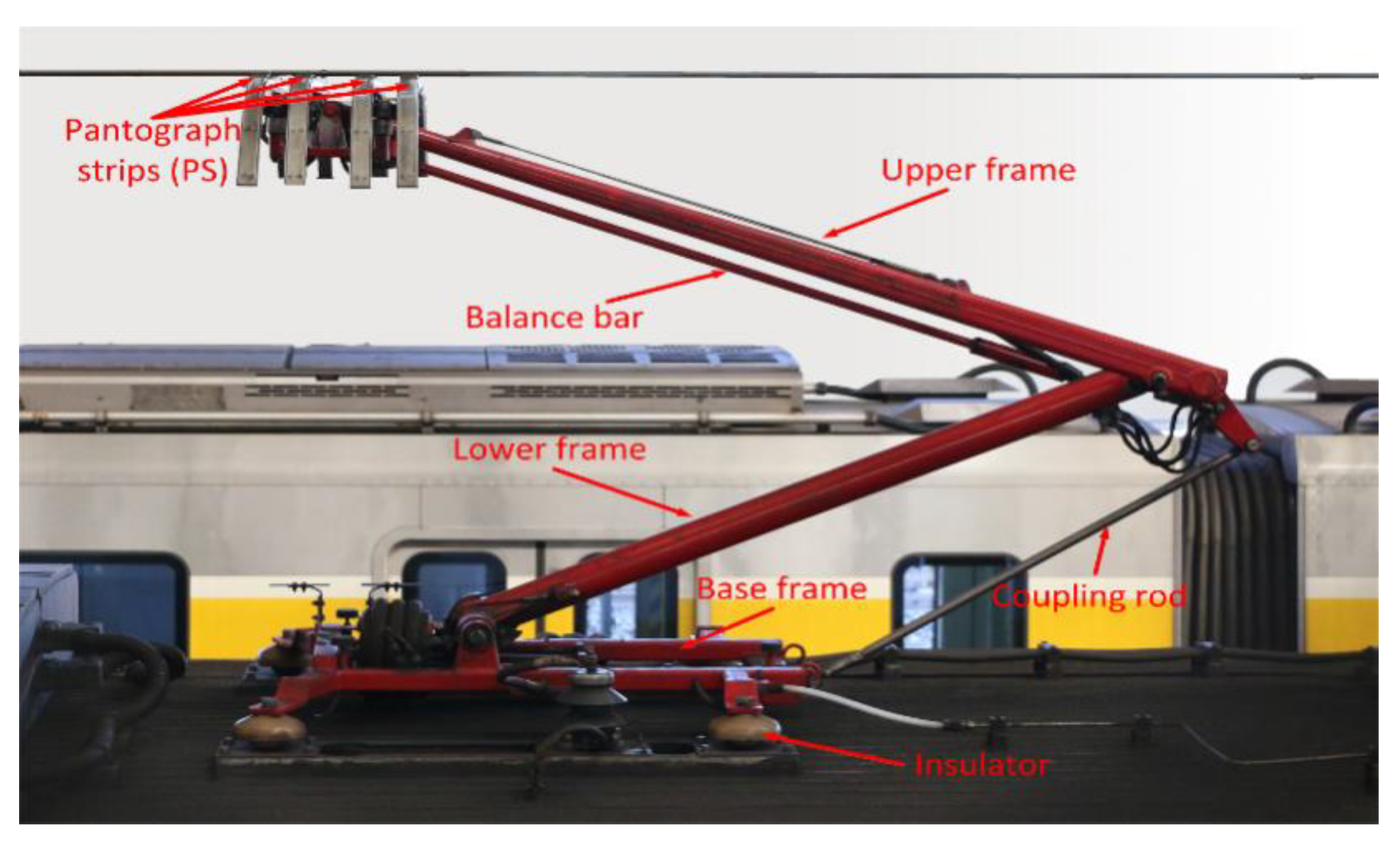
2.1. The Pantograph Carbon Contact Strip

Every subway has a total of two sets of pantographs (single-arm) which are installed on the odd number terminal and even number terminal, respectively. A typical single-arm pantograph for the subway system is shown in Figure 1. The overhead line is staggered for the track in order to guarantee uniform contact strip wear. The PCCS (see Figure 1) is located at the top of the pantograph head. It can clearly be seen that there are four carbon strips on the pantograph in contact with the catenary. If the train operates regularly, the four PCCSs contact with the catenary directly. If the pantograph lifting holding force is under the standard value, the carbon strip and catenary will not cooperate well, which may cause the arc discharge phenomenon due to the separation of carbon strip and catenary during operation, resulting in abrasion of the carbon strip and the catenary. The operation stability may influence the contacting force between one PCCS and the catenary. The overhead line slides over the carbon contact strips from one side to the other side repeatedly. The PCCS gets thinner and thinner gradually due to the wear issue between the catenary and the pantograph.

The thickness of the pantograph strip of a brand-new pantograph is around 40 mm for the one used in this application. In terms of the Pantograph Maintenance Manual, if the PCCS itself does not have any cracks, it is replaced according to the wear thickness. When the carbon contact strip is thinner than 4.5 mm, the PCCS must be replaced. This inspection work is still carried out by the maintenance staff periodically. It is very desirable to predict the RUL of the PCCS in time so that predictive maintenance can be carried out. For an illustrative purpose, an illustration of wear condition for PCCS is demonstrated in Figure 2.

In Figure 2, 40 mm represents the original thickness value, T1 and T2 are the remaining thickness value, the wear loss of the PCCS is the original thickness value minus the smallest value between T1 and T2 (the smallest remaining thickness value is taken as the record standard in practical).

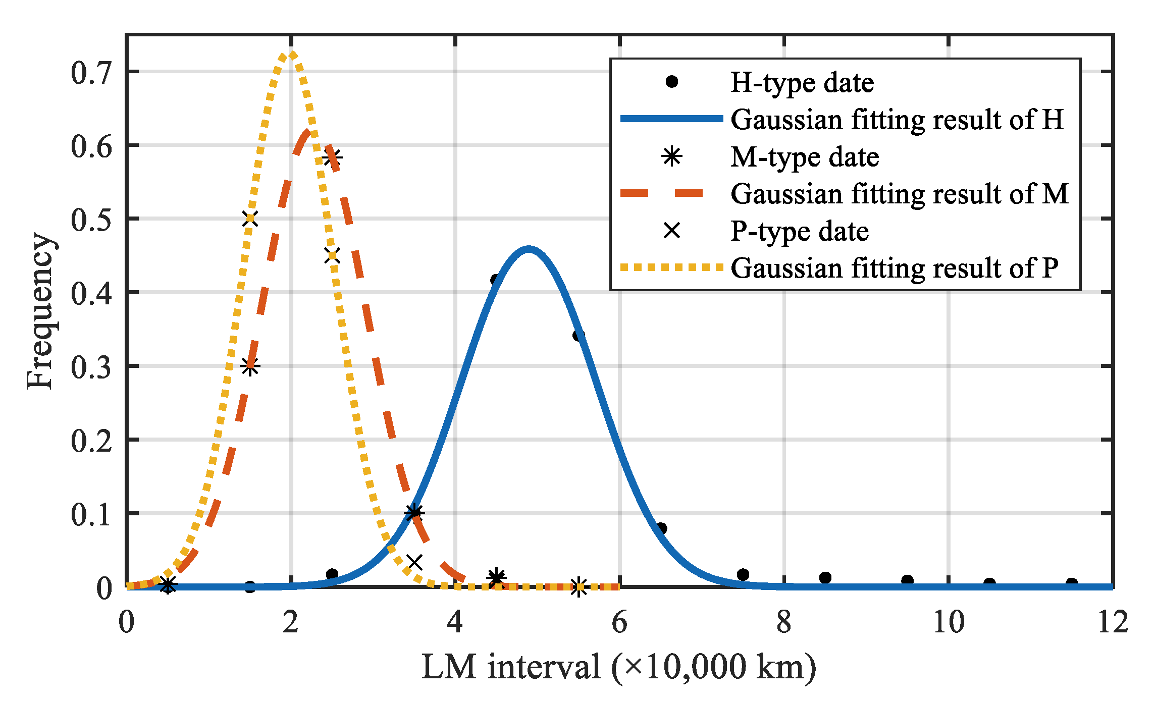
2.2. The Life Mileage Analysis of PCCS

In this section, life mileage (LM) of PCCS at Guangzhou Metro is analyzed. Three types of PCCS are used in Guangzhou Metro, including H-type, M-type and P-type, which are installed on the odd number terminal and even number terminal. H type is a metal impregnated material. M- and P-types are the all-carbon carbon strips. A total of 720 sets of wear data in the even number terminal are used for the LM analysis. Among the 720 data sets, 240 data sets are for the LM analysis of H-, M- and P-type PCCS, respectively.

The PCCS of each type have the ended life cycle of specific kilometers, which is called LM. The LM of each type PCCS is divided into twelve LM intervals, which take ten thousand kilometers as unit and begin from zero to twelve. The number of each type of PCCS in the intervals are shown in

Table 1. The number of three types for PCCS in the LM interval.

Type	LM Interval (×10,000 km)
	[0,1)	[1,2)	[2,3)	[3,4)	[4,5)	[5,6)	[6,7)	[7,8)	[8,9)	[9,10)	[10,11)	[11,12)
H type number	0	0	4	24	100	82	19	4	3	2	1	1
M type number	1	72	140	24	3	0	--	--	--	--	--	--
P type number	1	120	108	8	2	--	--	--	--	--	--	--

.

It can be seen from Table 1, the LM of the three types for the PCCS are quite different. H type PCCS has a much longer LM than the other two types. M-type and P-type have similar LM. The histogram of these three types of PCCS is shown in Figure 3.

Figure 3 demonstrates the LM for the three types of PCCS intuitively. The LM of these three types of PCCS from large to small is H-, M-, and P-type. The LM statistical distributions of the three types are assumed as Gaussian distribution according to Figure 3. The fitting results are described in Figure 4. The goodness of fit for the Gaussian distribution of the three types of PCCS are statistically analyzed. The statistical results are shown in

Table 2. The goodness of fit for the Gaussian distribution of the three types of PCCS.

Type	SSE	Adjusted R-Square	RMSE
H	8.7326e−4	0.9952	0.0099
M	2.0689e−4	0.9987	0.0083
P	6.5990e−4	0.9962	0.0148

. It should be noted that the closer the sum of squares due to error (SSE) is to zero, the better model fitting, and the more successful data prediction. Root mean squared error (RMSE) and SSE have the same effect. The typical value range of degree-of-freedom adjusted coefficient of determination (called Adjusted R-square) is [0, 1], and the closer it is to 1, the better the model fits the data.

The goodness of fit results in

Table 3. LM statistical results of the three types of PCCS.

Sample Parameter	Average	Maximum	Minimum	Standard Deviation
H	5.7691	11.1411	2.2022	1.6709
M	2.6948	5.0949	1.0311	0.6817
P	2.3689	4.1328	1.0092	0.6605

indicate that the Gaussian distribution fit the LM distribution of the three types of PCCS well. The statistical LM results are shown in Table 3, and the histogram of the average LM distribution of PCCS is shown in Figure 5.

Table 3 shows that the average LM for the three types of PCCS is quite different. For the same type, the LM is also with a significant distinction. For instance, for the H-type, the longest LM is 11.14 which is almost five times longer than the shortest LM 2.2. Therefore, the LM cannot be determined by the statistical distribution directly. Each type of PCCS has its own LM and should be estimated accurately. Figure 5 demonstrates the average of H-, M-, and P-types intuitively.

2.3. The Wear Development Trends Analysis of PCCS

Same as in Section 2.2, PCCS data are collected from forty-nine trains and from different seasons and times. The inspectors measure the data of PCCS on site, and there are at least two inspectors complete the maintenance related work. The PCCS should be inspected every week. The time of the inspect is not fixed. The recording interval of the data is not equal. Several data are used to analyze the wear development trends analysis of PCCS in every LM interval. Figure 6 shows the wear development trends of the three different types of PCCS.

2.4. Problem Statement

PCCS is a critical component of railway vehicles. It is desirable to know its RUL after one inspection is carried out. As stated in Section 2.3, the wear trend for each PCCS is distinctive. Therefore, RUL prediction is necessary for determining the maintenance and also inventory control, which motivates the work in this paper.

The Wiener process is widely used for the modeling of linear degradation process with random noise. A major advantage of the method is its sound mathematical characteristics. The standard BM-driven stochastic model can not only model the non-monotonic degradation process but also model the monotonic degradation process approximately, which has great flexibility. The method proposed in [8] is chosen because of its several attractive features: the degradation coefficient is update recursively by the KF algorithm; the EM algorithm is adopted to update the model parameters, and the exact PDF of the RUL is deduced based on FHT.

The standard method in [8] uses equal-interval data and the degradation process of the gyros has the non-monotonic. Because of the flexibility of the standard BM-driven stochastic model, the Wiener process can be used to model the monotonic degradation process of PCCS approximately. However, the wear inspection data is usually unequal interval data. Therefore, the problem to be solved is how to use the unequal interval data with the method in [8] to predict the RUL. This issue will be addressed in the following section first.

3. A Wiener Process-Based Approach of RUL Prediction with Unequal Interval Data

In this section, the RUL prediction method in [8] is extended to unequal interval data. Firstly, the method of unit time difference coefficient [14] is applied to deal with the unequal interval data. After that, the algorithm in [8] is briefly reviewed. After that, the EM algorithm is adopted to estimate the model parameters. Finally, the UIWGLRCM is introduced to restore the model parameters estimation.

The wear of the PCCS is recorded based on the mileage (km) the train has run. In this paper, it is assumed that the PCCSs are used under the same average train velocity; the mileage is used to describe the time scale; the mileage variable is equal as the time variable. In practice, the average velocity for each train is almost the same. Therefore, the assumption is acceptable. In practical application, the wear of PCCS depends on a univariate time scale, and the running miles are used to describe the wear process of PCCS. In this paper, the mileage is taken as the time scale variate. The notations used in the modeling process are described as nomenclature in Appendix A.

3.1. Preprocessing of Unequal Interval PCCS Wear Series

The method of unit time difference coefficient [14] is used to deal with the unequal interval data, to correct the deviation after unequal interval series are converted into equal interval series. The details are as follows.

The original unequal interval wear series are given:

$$\left\{Z^{\left(0\right)}({\tau }_1),Z^{\left(0\right)}({\tau }_2),\dots ,Z^{\left(0\right)}({\tau }_k)\right\},\hspace{0.17em}(k=1,2,\dots ,n)$$

(1)

where Z⁽⁰⁾(τ_k) = Z(τ_k), τ_k is unequal interval mileage point, Z(τ_k) is the wear loss at τ_k.

The actual mileage interval of the original unequal interval wear series at each monitored mileage point:

$$\Delta {\tau }_k={\tau }_k-{\tau }_{k-1}$$

(2)

The average mileage interval of monitoring mileage points:

$$\Delta {\tau }_0=\frac{{\tau }_n-{\tau }_1}{n-1}$$

(3)

Equal interval mileage points:

$${{\displaystyle T}}_{1:k}=\left\{0,\Delta {\tau }_0,2\Delta {\tau }_0,\dots ,(k-1)\Delta {\tau }_0\right\},\hspace{0.17em}(k=1,2,\dots ,n)$$

(4)

The unit mileage difference coefficients between every mileage segment and average mileage segment:

$$U({\tau }_k)=\frac{{\tau }_k-(k-1)\Delta {\tau }_0}{\Delta {\tau }_0},\hspace{0.17em}(k=1,2,\dots ,n)$$

(5)

The total difference of every actual mileage segment:

$$\Delta x^{\left(0\right)}({\tau }_k)=U({\tau }_k)[Z^{\left(0\right)}({\tau }_k)-Z^{\left(0\right)}({\tau }_{k-1})],\hspace{0.17em}(k=1,2,\dots ,n)$$

(6)

Equal mileage interval wear series:

$$X^{\left(0\right)}(T_k)=x^{\left(0\right)}({\tau }_k)-\Delta x^{\left(0\right)}({\tau }_k),\hspace{0.17em}(k=1,2,\dots ,n)$$

(7)

where X⁽⁰⁾(T_k) = X(T_k), X(T_k) is the wear loss at equal interval mileage points T_k.

After converting the unequal interval wear series to equal interval series, a linear wear model based on the equal interval wear series can be established.

3.2. Linear Random Wear Modeling and RUL Prediction

In this article, a linear wear model is established based on the Wiener process. The random wear process X(T) is described as:

$$X({\rm T})=X\left(0\right)+\theta T+\sigma B\left(T\right)$$

(8)

where θ is the coefficient of wear rate, σ is the diffusion coefficient, X(0) is the initial wear loss, B(T) is standard BM. In general, X(0) = 0.

In order to predict the RUL of the device accurately, the FHT [15] is used to define the life of the device. X_0:k = X(T_0:k) indicates the wear series of PCCS at T_k. The RUL of PCCS is defined as:

$${{\displaystyle L}}_k=\inf \left\{{{\displaystyle l}}_k:X({{\displaystyle l}}_k+{{\displaystyle {\rm T}}}_k)\ge w|{{\displaystyle X}}_{0:k}\right\}$$

(9)

where w is failure threshold, X_0:k = {X₀,X₁,X₂,…,X_k} is the wear loss at T_k.

The model assumptions are widely used in [6,16,17,18,19,20,21]. In this paper, the assumptions are as follows:

(1) θ is a Gaussian distribution, which satisfies $\theta =N({\mu }_{\theta },{{\displaystyle \sigma }}_{\theta }^2)$,

(2) θ and B(T) are mutually independent.

The initial wear rate coefficient θ is assumed ${\theta }_0=N(\mu ,{{\displaystyle \sigma }}_{\theta }^2)$. In most methods of RUL prediction, the estimation of the parameters at the current monitoring point is assumed exactly equal to the posterior estimations of the previous monitoring point. In this assumption, the state equation and observation equation based on state-space models [22] are described as:

$$\begin{array}{l}{\theta }_k={\theta }_{k-1}+{\omega }_k\\ X_k=X_{k-1}+{\theta }_{k-1}(T_k-T_{k-1})+{\upsilon }_{k-1}\end{array}$$

(10)

where ω and υ are random error terms, ${\omega }_k~N(0,Q)$,${{\displaystyle \upsilon }}_{k-1}=\sigma (B({{\displaystyle {\rm T}}}_k)-B({{\displaystyle {\rm T}}}_{k-1}))$, ${\upsilon }_{k-1}~N(0,{{\displaystyle \sigma }}^2({{\rm T}}_{k-1},{{\rm T}}_{k-1}))$ is obtained according to the characteristics of standard BM.

In this article, θ_k is a hidden variable. The Bayesian rule is used to recursively update the estimation of probability distribution under X_0:k. The expectation and variance of the posterior estimation of θ at T_k are defined as:

$$\begin{array}{l}{{\displaystyle \widehat{\theta }}}_{k|k}=E({{\displaystyle \theta }}_k|{{\displaystyle X}}_{0:k})\\ {{\displaystyle P}}_{k|k}=\mathrm{var}({{\displaystyle \theta }}_k|{{\displaystyle X}}_{0:\mathrm{k}})\end{array}$$

(11)

The KF [22] is used to estimate the variables in the Equation (11) based on the Equation (10) and X_0:k. Furthermore, in the KF process, the equation ${{\displaystyle \widehat{X}}}_{{}_{k+1}}={{\displaystyle X}}_k+{{\displaystyle \widehat{\theta }}}_{{}_{k+1}}({{\displaystyle T}}_{k+1}-{{\displaystyle T}}_k)$ is used to predict the wear path by one-step. KF algorithm is well known and it will not be repeated here.

According to the wear data X_0:k, the Equations (8), (9) and (11), the PDF of RUL prediction for PCCS is:

$$f_{L_k|X_{1:\mathrm{k}}}({{\displaystyle l}}_k|X_{0:\mathrm{k}})=\frac{w-X_k}{\sqrt{2\pi {{\displaystyle l}}_k^3({{\displaystyle P}}_{k|k}{{\displaystyle l}}_k+{\sigma }^2)}}\exp [-\frac{{(w-X_k-{{\displaystyle \widehat{\theta }}}_{k|k}{{\displaystyle l}}_k)}^2}{2l_k({{\displaystyle P}}_{k|k}{{\displaystyle l}}_k+{\sigma }^2)}],\hspace{0.17em}{l}_k>0$$

(12)

The Equation (12) has a detailed proof process in [8], it will not be repeated here. It can be seen that the RUL distribution predicted by the method in this article is an exact closed solution. The expectation of RUL prediction is described as:

$$\begin{array}{l}E({{\displaystyle L}}_k|{{\displaystyle X}}_{0:k})=E(\frac{w-X_k}{\theta }|{{\displaystyle X}}_{0:k})=\frac{w-X_k}{{{\displaystyle P}}_{k|k}}\exp (-\frac{{{\displaystyle \widehat{\theta }}}_{k|k}}{2{{\displaystyle P}}_{k|k}}){\displaystyle {\int }_0^{{{\displaystyle \widehat{\theta }}}_{k|k}}\exp (-\frac{{{\displaystyle u}}^2}{2{{\displaystyle P}}_{k|k}})}\\ =\frac{\sqrt{2}(w-X_k)}{\sqrt{{{\displaystyle P}}_{k|k}}}D(\frac{{{\displaystyle \widehat{\theta }}}_{k|k}}{\sqrt{2{{\displaystyle P}}_{k|k}}})\end{array}$$

(13)

where $D(z)=\exp (-{{\displaystyle z}}^2){\displaystyle {\int }_0^z\exp ({{\displaystyle u}}^2)}du$ is Dawson integral. In particular, if Pr(θ < 0) = 0, the D(z) ≈ 1/2z, then $E({{\displaystyle L}}_k|{{\displaystyle X}}_{0:k})=(w-{{\rm X}}_k)/{{\displaystyle \widehat{\theta }}}_{k|k}$.

The model parameters ${\mu }_{\theta },{{\displaystyle \sigma }}_{\theta }^2,Q,{\sigma }^2$ are unknown. In order to obtain a more accurate RUL prediction for PCCS, the wear data X_0:k are used to update the model parameters continuously.

3.3. Model Parameters Estimation

In this article, the unknown model parameters are donated by a vector; the vector is written as $\Theta ={[{\mu }_{\theta },{{\displaystyle \sigma }}_{\theta }^2,Q,{\sigma }^2]}^{\mathrm{T}}$. The log-likelihood function of X_0:k at T_k for Θ is expressed as:

$${{\displaystyle L}}_k(\Theta )=\ln [p({{\displaystyle X}}_{0:k}|\Theta )]$$

(14)

where p(X_0:k|Θ) is the joint PDF of X_0:k for Θ. The maximum likelihood estimation of Θ based on L_k(Θ) is formulated by:

$${{\displaystyle \widehat{\Theta }}}_k=\arg \underset{\Theta }{{\displaystyle \max }}{{\displaystyle L}}_k(\Theta )$$

(15)

In this paper, θ is a hidden variable. Therefore, it is difficult to maximize the Equation (14) directly. The EM algorithm [23] is used to solve this problem. The following two steps can achieve the estimation of Θ:

(1)

E-step

$$\ell (\Theta |{\widehat{\Theta }}_k^{(i)})={{\displaystyle \mathbb{E}}}_{{\theta }_k|X_{0:k},{\widehat{\Theta }}_k^{(i)}}\{\ln p({{\displaystyle X}}_{0:k},{{\displaystyle \theta }}_k|\Theta )\}$$

(16)

where ${\widehat{\Theta }}_k^{(i+1)}={[({\mu }_{\theta })}_k^{(i)},{({{\displaystyle \sigma }}_{\theta }^2)}_k^{(i)},{(Q)}_k^{(i)},{({\sigma }^2)}_k^{(i)}{]}^{\mathrm{T}}$ is the result in the ith iteration based on X_0:k.

(2)

M-step

$${\widehat{\Theta }}_k^{(i+1)}=\arg \underset{\Theta }{{\displaystyle \max }}\{\ell (\Theta |{\widehat{\Theta }}_k^{(i)})\}$$

(17)

The EM algorithm needs to iterate many times. Generally, the iteration is terminated when the difference between $\ell (\Theta |{\widehat{\Theta }}_k^{(i)})$ and $\ell (\Theta |{\widehat{\Theta }}_k^{(i+1)})$ is less than a small value. A series of optimal estimation of model parameters are obtained through the iterative process; the model parameters are denoted by $\{{\widehat{\Theta }}_k^{(0)},{\widehat{\Theta }}_k^{(1)},\dots ,{\widehat{\Theta }}_k^{(i)},{\widehat{\Theta }}_k^{(i+1)}\}$. The details of the EM algorithm and realization are summarized in Appendix B. The convergence property of the EM algorithm has a detailed demonstration in [8]. It will not be repeated here.

3.4. Restoration of Model Parameter and Wear Loss

The estimated parameters in Section 3.2 need to be reversed to the original value at unequal interval mileage points. In this paper, the UIWGLRCM in [24] is applied to restore the estimation of the parameters.

The estimated optimal parameters are ${\widehat{\Theta }}_k^{(i+1)}=[{({{\displaystyle \widehat{\mu }}}_{\theta })}_k^{(i+1)},{({{\displaystyle \widehat{\sigma }}}_{\theta }^2)}_k^{(i+1)},{(\widehat{Q})}_k^{(i+1)},{({{\displaystyle \widehat{\sigma }}}^2)}_k^{(i+1)}{]}^{\mathrm{T}}$ through the EM algorithm. The wear loss estimates ${{\displaystyle \widehat{X}}}_{1:k}$ are obtained by one-step prediction in the KF process. $({{\displaystyle \widehat{\mu }}}_{\theta }{)}_k^{(i+1)}$ is used to describe the proposed model in detail, let $x_{1:k}={({{\displaystyle \widehat{\mu }}}_{\theta })}_{1:k}^{(i+1)}$.

The original parameter series of equal mileage intervals is given as:

$$x^{\left(0\right)}(k)=\left\{x^{\left(0\right)}(1),x^{\left(0\right)}(2),\dots ,x^{\left(0\right)}(k)\right\},\hspace{0.17em}(k=1,2,\dots ,n)$$

(18)

where $x^{\left(0\right)}(1:k)=x_{1:k},\hspace{0.17em}(k=1,2,\dots ,n)$.

The original parameter series of equal mileage intervals is accumulated once, the series is written as:

$$x^{\left(1\right)}(k)=\left\{x^{\left(1\right)}(1),x^{\left(1\right)}(2),\dots ,x^{\left(1\right)}(k)\right\},\hspace{0.17em}(k=1,2,\dots ,n)$$

(19)

where $x^{\left(1\right)}(k)={\displaystyle \sum _{j=1}^k{x}^{\left(0\right)}(j)},\hspace{0.17em}(k=1,2,\dots ,n)$.

According to the principle of the classical grey model (GM) [25], the response equation of equal interval GM (1,1) is formulated by:

$${{\displaystyle \widehat{x}}}^{(1)}(k+1)=(x^{(0)}(1)-b/a)\exp (-ak)+b/a$$

(20)

where a denotes development coefficient, b is grey action, they are calculated according to the principle of the least square method.

The form of the Equation (20) can be written as:

$${{\displaystyle \widehat{x}}}^{(1)}(k+1)={{\displaystyle C}}_1\exp (vk)+{{\displaystyle C}}_2$$

(21)

The linear regression equation Y = aX + b and exponential equation Y = ae^X are used to fit the accumulation series. The series is formulated by:

$${{\displaystyle \widehat{x}}}^{(1)}(k+1)={{\displaystyle C}}_1\exp (vk)+{{\displaystyle C}}_{2}k+{{\displaystyle C}}_3$$

(22)

where C₁, C₂, C₃, and v are all unknown, they need to be estimated.

C₁, C₂, C₃ and v are assumed to have a relationship of the Equation (23):

$$\begin{array}{l}L(k)={{\displaystyle \widehat{x}}}^{(1)}(k+1)-{{\displaystyle \widehat{x}}}^{(1)}(k)\\ ={{\displaystyle C}}_1\exp (vk)[\exp (v)-1]+{{\displaystyle C}}_2\end{array}$$

(23)

$Y_{\mathrm{m}}(k)=L(k+m)-L(k)$ is assumed to calculated v, v is written as:

$$v=\ln [Y_{\mathrm{m}}(k+1)/Y_{\mathrm{m}}(k)]$$

(24)

The approximations of v in the Equation (24) are obtained by replacing ${\widehat{x}}^{(1)}(k)$ as $x^{(1)}(k)$, the average approximations are taken as the estimation of v, which are obtained by:

$$\widehat{v}=2{\displaystyle \sum _{m=1}^{n-3}{\displaystyle \sum _{k=1}^{n-2-m}{v}_m(k)}}/[(n-2)(n-3)]$$

(25)

The value of different mileage points in the original data series should be assigned a weight to represent its reliability, and the weight increases exponentially with time. The weight matrix is formulated by:

$$p=diag({{\displaystyle R}}^{n-1})$$

(26)

where R is weight increasing factor, generally the value range of w is from 1 to 2. In this article, R = 1.5.

According to the Equation (26), the least squares is used to calculate C:

$$\mathrm{C}={{(\mathrm{A}}^{\mathrm{T}}p\mathrm{A})}^{-1}{\mathrm{A}}^{\mathrm{T}}p{{\displaystyle \widehat{X}}}^{(1)}$$

(27)

where $C=\left[\begin{array}{l}{{\displaystyle C}}_1\\ {{\displaystyle C}}_2\\ {{\displaystyle C}}_3\end{array}\right]$, ${{\displaystyle \widehat{X}}}^{(1)}=\left[\begin{array}{c}{{\displaystyle \widehat{X}}}^{(1)}(1)\\ {{\displaystyle \widehat{X}}}^{(1)}(2)\\ ⋮\\ {{\displaystyle \widehat{X}}}^{(1)}(n)\end{array}\right]$, $A=\left[\begin{array}{ccc}{e}^v& 1& 1\\ e^{2v}& 2& 1\\ ⋮& ⋮& ⋮\\ e^{3v}& n& 1\end{array}\right]$.

The UIWGLRCM is written as:

$${{\displaystyle \widehat{x}}}^{(1)}(\tau )=C_1\exp [v(\tau /\Delta {\tau }_0+1)]+C_2(\tau /\Delta {\tau }_0+1)+C_3$$

(28)

where τ is the mileage interval which distances from the first cycle, τ = τ_k-Δτ₀.

Through once inverse accumulated, the unequal interval wear series is formulated by:

$$\{\begin{array}{l}{{\displaystyle \widehat{x}}}^{(0)}(\tau )={{\displaystyle \widehat{x}}}^{(0)}(\tau ),\hspace{0.17em}\tau =0\\ {{\displaystyle \widehat{x}}}^{(0)}(\tau )={{\displaystyle \widehat{x}}}^{(1)}(\tau )-{{\displaystyle \widehat{x}}}^{(1)}(\tau -\Delta {\tau }_0),\hspace{0.17em}\tau >0\end{array}$$

(29)

The flow chart of the RUL prediction method proposed in this article is shown in Figure 7. The estimated parameters and the prediction of wear loss after the KF algorithm are restored by the Equation (29). The PDF of the RUL prediction is calculated by the Equation (12), and the expectation of the RUL prediction is obtained by the Equation (13).

4. Cases Study

4.1. Data Description

The thickness of the PCCS determines whether it should be replaced or not. When the lower limit of the PCCS is reached, maintenance needs to be scheduled to replace it with a new one. The initial thickness minus the minimum required thickness 4.5 mm is taken as the failure threshold of the PCCS.

The wear data are collected from the Guangzhou Metro. The wear value is recorded by the mileage (km) the train runs. The collected wear data are unequal intervals since the inspection interval of the PCCS is not fixed strictly. Here the H-type PCCS is taken as an example to demonstrate the proposed method. The wear development trends of 12 samples for H-type PCCS are illustrated in Figure 8.

As is shown in Figure 8, the wear development trends of the twelve samples are similar, but the wear rates are very different. In this paper, two PCCS samples (as marked in the plot) with large differences in wear rates are selected for this case study. The selected wear data of PCCS are shown in

Table 4. The selected wear data for PCCS.

Category	Original Thickness mm	Thickness of the Last Point mm	Original Mileage 1000 km	Mileage of the Last Point 1000 km	LM 1000 km
Sample 1	18.5	4.6	850.786	893.473	42.687
Sample 2	19.10	4.7	1394.295	1504.763	110.468

. The wear loss (Z(τ_k)) is obtained by using the original thickness minus the thickness of each point. The running miles as the unequal interval mileage point (τ_k) are given by using the original mileage minus the mileage of each mileage point. The original unequal interval wear series are taken as the input. Then the proposed method is used to predict the wear loss at a specific point and the prediction of the remaining useful mileage life. Furthermore, the estimation of the parameters, PDF of the RUL, and other related parameters are also obtained.

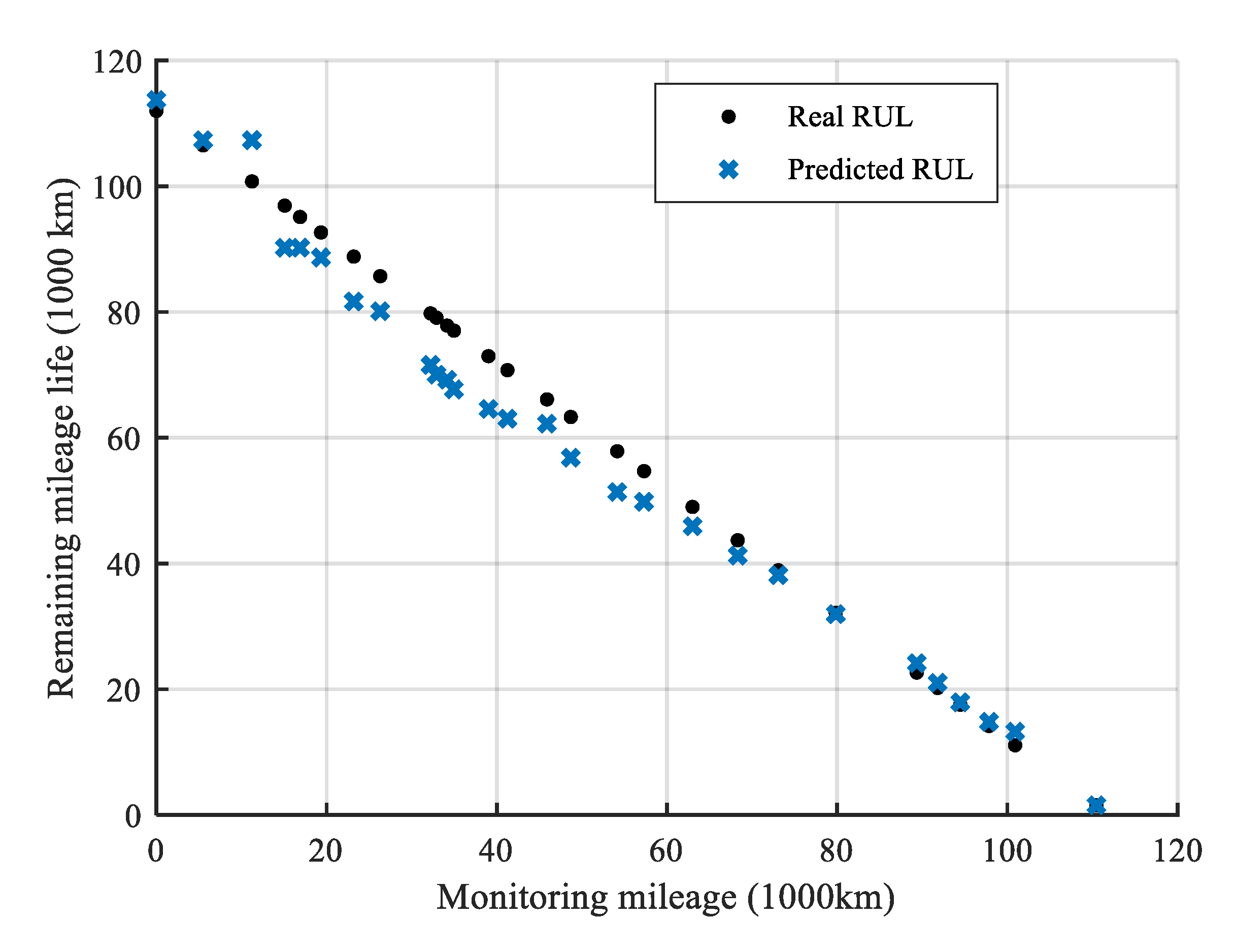
4.2. RUL Prediction of PCCS

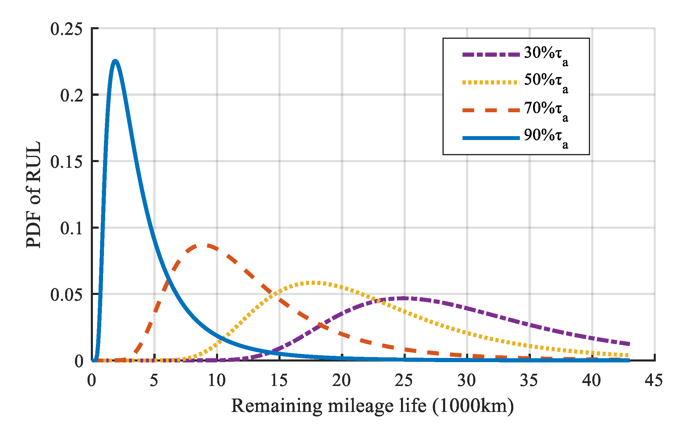
4.2.1. The RUL Prediction of Sample 1

In light of the PCCS maintenance requirement, the failure threshold of Sample 1 is w = 14 mm and the actual failure LM L_fail = 43 thousand kilometers. Fourteen mileage points are recorded. The inspection of mileage intervals are unequal. Firstly, the unequal interval wear series are converted to equal interval series. Figure 9 shows the result of the conversion process of unequal interval wear series to equal interval ones.

In order to calculate the prediction of the wear rate coefficient and the PDF distribution of the RUL prediction for the PCCS at each mileage point, firstly, the initial model parameters are taken as Θ = [0.3,0.2,0.01,0.1]^T, the equation ${{\displaystyle \widehat{X}}}_{{}_{k+1}}={{\displaystyle X}}_k+{{\displaystyle \widehat{\theta }}}_{{}_{k+1}}({{\displaystyle T}}_{k+1}-{{\displaystyle T}}_k)$ is used to predict the wear path by one-step, and then, the predicted results are restored by Equation (29). The predicted wear trend of the proposed method and the actual wear path are shown in Figure 10.

It can be seen from Figure 10 that the predicted wear loss is very close to the actual wear loss. The mean squared error (MSE) of the predicted wear and the actual wear at each mileage point is used to assess the prediction results. The MSE index at each monitoring mileage point τ_k is defined by:

$${\displaystyle MSE}(k)={\displaystyle \sum _{i=1}^k{{\displaystyle [Z({\tau }_k)-{{\displaystyle Z}}_{pre}({\tau }_k)]}}^2/k}$$

(30)

where Z_pre(τ_k) is the restored wear loss at τ_k after one-step prediction.

The MSE of Sample 1 at each mileage point is illustrated in Figure 11.

The average MSE between the actual wear and predicted wear is 0.0047 which is small. For example, at the last mileage point MSE(14) = 0.0041, the prediction result is very good, which demonstrates that the proposed model can predict the wear of the PCCS very well.

In order to demonstrate the prediction ability of the proposed method, the PDF of RUL at life quantiles of 30%, 50%, 70%, and 90% are applied to compare the results, τ_k∈{0.30τ_a, 0.50τ_a, 0.70τ_a, 0.90τ_a}, where τ_a is the actual LM of the PCCS. The prediction results are shown in Figure 12.

Figure 12 shows that the PDF of the RUL becomes narrower with the accumulation of wear data. Hence it indicates that the prediction result is better and better.

The relative error (RE) between the real and predicted RUL is adopted as a performance measure of prediction ability. The RE at each monitoring mileage point τ_k is formulated by:

$$RE(k)=|L_{real}({\tau }_k)-E_{pre}({\tau }_k)|/L_{real}({\tau }_k)$$

(31)

where L_real(τ_k) is the real RUL, here L_real(τ_k) = L_fail-τ_k, E_pre(τ_k) is the expectation of RUL prediction at τ_k.

The RE of Sample 1 is calculated by the Equation (31). The illustration of the results is given in Figure 13.

In Figure 13, it can observe that the RE at the last three mileage point exceeds 0.1, but the RE of the other mileage points are smaller than 0.1. At the last mileage point, the RE(14) = 0.0083. It indicates that the proposed method in this paper is feasible.

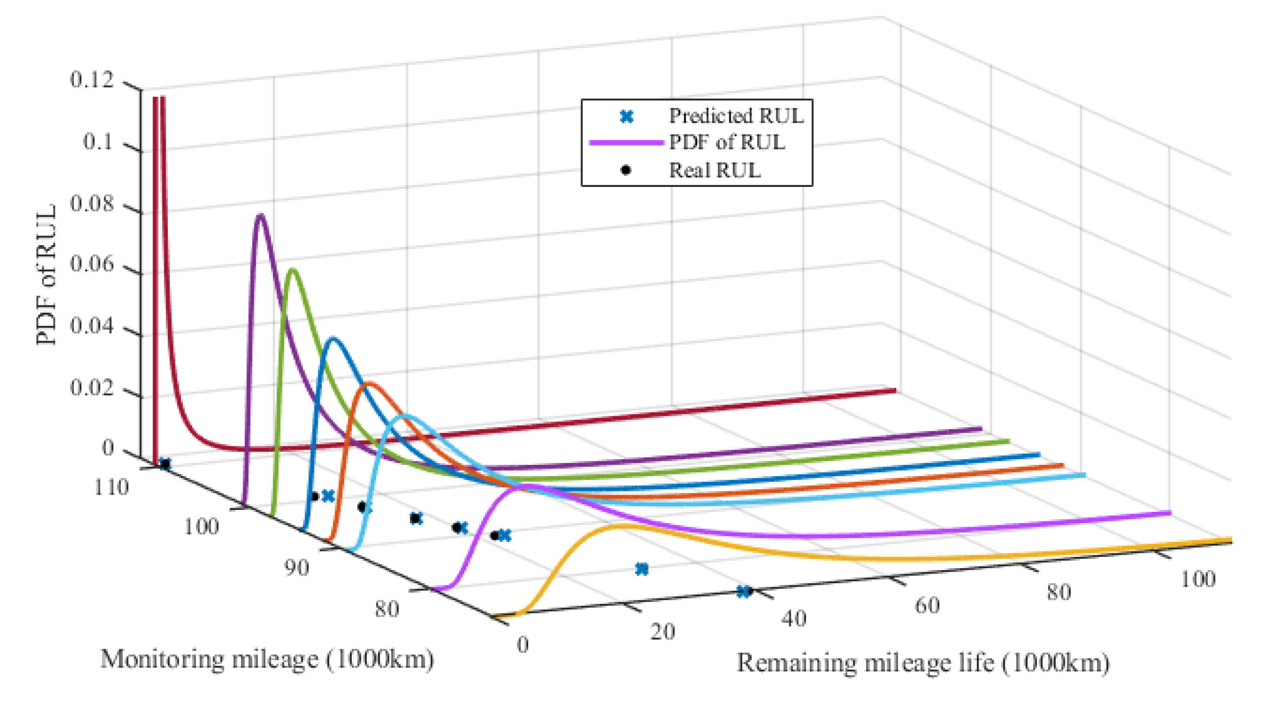
4.2.2. The RUL Prediction Result of Sample 2

The failure threshold of Sample 2 is w = 14.6, the actual failure LM L_fail = 112 thousand kilometers, and the initial parameters are given as Θ = [0.12,0.6,0.01,0.1]^T, the predicted and actual wear path of sample 2 are shown in Figure 14.

Figure 14 shows that the predicted wear trend is very close to the actual wear loss, and the average MSE between the actual predicted wear is 0.0597, which is small. It proves that the proposed model can fit the wear loss well. The EM algorithm is applied to estimate the model parameter. The restoration results of estimation at each mileage point are shown in Figure 15.

Figure 15 demonstrates that the model parameters can converge quickly with the wear data accumulates. The model parameters can be updated at each mileage point, and then the PDF of the RUL is calculated by the Equation (12). The PDF of RUL prediction at the last eight monitoring points is shown in Figure 16.

As is shown in Figure 16, every real RUL point falls within the PDF of the RUL, and the PDF curves become narrower with wear data information increases, which indicates the result of RUL prediction is more and more accurate.

In order to validate the performance of the proposed method, the prediction result is compared to the real RUL at each mileage point. The results are shown in Figure 17.

Figure 17 shows that the result of the RUL prediction is very close to the real RUL. The average RE between the real RUL and predict RUL is 0.0702. For example, the RE at the last mileage point is 0.0170. It shows that the RUL prediction of PCCS is very precise.

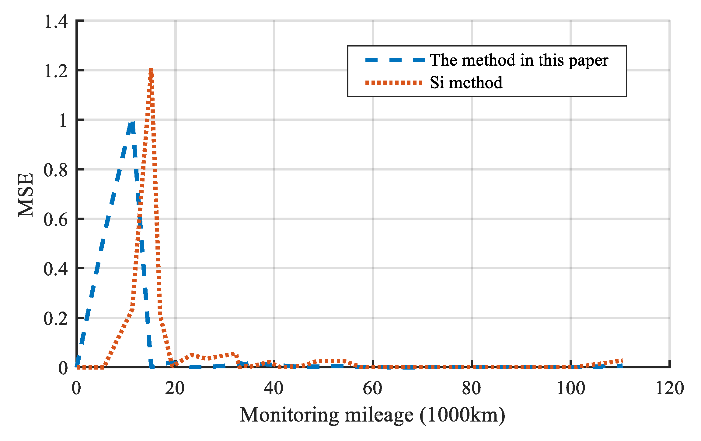
4.3. Comparative Study

A comparative study is set up to validate the effectiveness and advantages of the proposed method in applications of unequal interval data. The method in [8] (it is called the Si method in the following) is used to compare the RUL prediction with the proposed method. The equation ${{\displaystyle \widehat{X}}}_{{}_{k+1}}={{\displaystyle X}}_k+{{\displaystyle \widehat{\theta }}}_{{}_{k+1}}({{\displaystyle T}}_{k+1}-{{\displaystyle T}}_k)$ is used to predict the wear path by one-step in the Si method. The predicted wear paths of the PCCS are obtained by the proposed method in this article. The actual wear path and predicted wear paths of two methods are shown in Figure 18.

It should be noted that the smaller the MSE, the higher the accuracy of the prediction of wear loss. The MSE of two methods at each mileage point is illustrated in Figure 19.

It can be seen that the method in this article has a higher accuracy of the prediction of wear loss than the one by Si method. At the last mileage point, the MSE(28) of the two methods is 0.0062 and 0.0272, respectively. It indicates that the algorithm proposed in this paper improves the accuracy of the prediction for the PCCS wear loss effectively.

It is essential to point out that the smaller the RE, the higher the accuracy of the prediction. The RE of RUL prediction at the life quantiles of 35%, 55%, 75%, and 95% are calculated to compare the RUL prediction performance of the two methods. The prediction results are shown in

Table 5. RUL Prediction and RE of the two methods.

Method	35% Quantile	55% Quantile	75% Quantile	95% Quantile
Si method	57.1711	40.6560	28.2535	1.3780
	(21.66%)	(17.02%)	(12.16%)	(10.05%)
Method of this paper	64.5765	45.9183	31.9183	1.5580
	(11.51%)	(6.28%)	(0.77%)	(1.70%)

.

As can be seen that in Table 5 the RE at the four quantiles of the method in this paper are smaller than the Si method. To intuitively describe the change of RE, the RE of the two methods at each mileage point is given in Figure 20.

Figure 20 shows that the RE of the method in this paper is smaller than the RE of the Si method. The average RE of the method in this paper and Si method are 0.0702 and 0.1514, respectively. It demonstrates that the method in this paper has a higher accuracy of the RUL prediction than the Si method. The performance of the RUL estimation of the two methods is illustrated in Figure 21.

It demonstrates that the proposed method of this article has distinct advantages compared with the Si method in Figure 21. For example, the real RUL is 1.5320 at the last mileage point, the predicted RUL of this paper and the Si method are 1.5580 and 1.3780, respectively. The corresponding absolute error is 0.0260 and 0.1540, respectively. At τ₂₈ = 110.4680, the RE of the two methods is 0.0170 and 0.1005, respectively. It shows that the method in this paper can effectively improve the accuracy of RUL prediction.

5. Conclusions

This paper focuses on the RUL prediction of the PCCS in the railway system. The LM distribution is analyzed in the first place. It shows that the wear development trend is distinctive for each PCCS, even for the same type of PCCS. After that, a Wiener-process-based RUL prediction method considering unequal data interval is proposed. Firstly, the method of unit time difference coefficient is applied to convert the unequal interval wear data into the equal interval ones which are used for wear modeling. Then, the model parameters are estimated by the EM algorithm, and the UIWGLRCM is introduced to restore the estimations of model parameters and the wear loss. Finally, the PDF and the prediction of RUL are obtained.

The proposed method is further applied to the RUL prediction issue of the PCCS. By comparing with the Si method (the method in [8]), the proposed method in this article achieves a more accurate prediction of wear path and RUL in considering the unequal interval wear data. So the proposed method has attractive features: the degradation coefficient is update recursively by the KF algorithm; the EM algorithm is adopted to update the model parameter; the exact PDF of the RUL is deduced based on FHT. The comparative study demonstrates that the proposed method is practical and achieves a better performance in solving the unequal interval problem. The improved method provides a practical alternative for the RUL prediction of the PCCS.

References

1. Petch, M. Prognostics and Health Management of Electronics; Wiley Online Library: Hoboken, NJ, USA, 2008. [Google Scholar]
2. Heng, A.; Zhang, S.; Tan, A.C.C.; Mathew, J. Rotating machinery prognostics: State of the art, challenges and opportunities. Mech. Syst. Signal Process. 2009, 23, 1600–1614. [Google Scholar] [CrossRef]
3. Sikorska, J.Z.; Hodkiewicz, M.; Ma, L. Prognostic modeling options for remaining useful life estimation by industry. Mech. Syst. Signal Process. 2011, 25, 1803–1836. [Google Scholar] [CrossRef]
4. Jardine, A.; Lin, D. A review on machinery diagnostics and prognostics implementing condition-based maintenance. Mech. Syst. Signal Process. 2006, 20, 1483–1510. [Google Scholar] [CrossRef]
5. Hu, C.; Zhou, Z.; Zhang, J.; Si, X. A survey on life prediction of equipment. Chin. J. Aeronaut. 2015, 28, 25–33. [Google Scholar] [CrossRef] [Green Version]
6. Gebraeel, N.; Lawley, M.; Liu, R.; Parmeshwaran, V. Residual life predictions from vibration-based degradation signals: A neural network approach. IEEE Trans. Ind. Electron. 2004, 51, 694–700. [Google Scholar] [CrossRef]
7. Wang, W.; Carr, M.; Xu, W.; Kobbacy, K. A model for residual life prediction based on Brownian motion with an adaptive drift. Microelectron. Reliab. 2011, 51, 285–293. [Google Scholar] [CrossRef]
8. Si, X.; Wang, W.; Hu, C.; Chen, M.; Zhou, D. A Wiener-process-based degradation model with a recursive filter algorithm for RUL estimation. Mech. Syst. Signal Process. 2013, 35, 219–237. [Google Scholar] [CrossRef]
9. Gao, Z.; Yin, X.; Zhang, B.; Chen, M.; Li, B. A Wiener process-based remaining life prediction method for light-emitting diode driving power in rail vehicle carriage. Adv. Mech. Eng. 2019, 11, 1–8. [Google Scholar] [CrossRef]
10. Hu, Y.; Li, H.; Shi, P.; Chai, Z.; Wang, K.; Xie, X. A prediction method for the real-time remaining useful life of wind turbine bearings based on the Wiener process. Renew. Energy 2018, 127, 452–460. [Google Scholar] [CrossRef]
11. Zhang, Z.; Si, X.; Hu, C.; Hu, X.; Sun, G. An adaptive prognostic approach incorporating inspection influence for deteriorating systems. IEEE Trans. Reliab. 2018, 68, 302–316. [Google Scholar] [CrossRef]
12. Tang, S.; Yu, C.; Wang, X.; Guo, X.; Si, X. Remaining useful life prediction of lithium-ion batteries based on the Wiener process with measurement error. Energies 2014, 7, 520–547. [Google Scholar] [CrossRef] [Green Version]
13. Zhang, Z.; Si, X.; Hu, C.; Lei, Y. Degradation data analysis and remaining useful life estimation: A review on wiener-process-based methods. Eur. J. Oper. Res. 2018, 271, 775–796. [Google Scholar] [CrossRef]
14. Yuan, J. Grey System Theory and Application; Science Press: Beijing, China, 1991; pp. 52–57. [Google Scholar]
15. Lee, M.; Whitmore, G. Threshold regression for survival analysis: Modeling event times by a stochastic process reaching a boundary. Stat. Sci. 2006, 21, 501–513. [Google Scholar] [CrossRef] [Green Version]
16. Meeker, W.; Escobar, L. Statistical Methods for Reliability Data; John Wiley & Sons Inc.: New York, NY, USA, 1998. [Google Scholar]
17. Gebraeel, N.; Elwany, A.; Pan, J. Residual life predictions in the absence of prior degradation knowledge. IEEE Trans. Reliab. 2009, 58, 106–117. [Google Scholar] [CrossRef]
18. Park, J.; Bae, S. Direct prediction methods on lifetime distribution of organic light-emitting diodes from accelerated degradation tests. IEEE Trans Reliab. 2010, 59, 74–90. [Google Scholar] [CrossRef]
19. Elwany, A.; Gebraeel, N.; Maillart, L. Structured replacement policies for components systems with complex degradation processes and dedicated sensors. Oper. Res. 2011, 59, 684–695. [Google Scholar] [CrossRef]
20. Wang, D.; Tsui, K. Brownian motion with adaptive drift for remaining useful life prediction: Revisited. Mech. Syst. Signal Process. 2018, 99, 691–701. [Google Scholar] [CrossRef]
21. Cai, Z.; Guo, J.; Chen, Y.; Dong, X.; Xiang, H. Remaining lifetime online prediction based on step-stress accelerated degradation modeling. Syst. Eng. Electron. 2018, 40, 2605–2610. [Google Scholar]
22. Harvey, A.C. Forecasting Structural Time Series Models and the Kalman Filter; Cambradge University Press: Cambridge, UK, 1989. [Google Scholar]
23. Dempster, A.P. Maximum likelihood from incomplete data via the EM algorithm. J. R. Stat. Soc. B 1977, 39, 1–38. [Google Scholar]
24. Li, B.; He, C. The combined forecasting method of GM(1,1) with linear regression and its application. In Proceedings of the IEEE International Conference on Grey Systems and Intelligent Services, Nanjing, China, 18–20 November 2007; pp. 394–398. [Google Scholar]
25. Deng, J. Control Problems of Grey Systems. Syst. Control Lett. 1982, 1, 288–294. [Google Scholar]
Figure 1. The pantograph of the metro vehicle.
Applsci 10 01616 g001
Figure 2. The carbon contact strip.
Applsci 10 01616 g002
Figure 3. The LM histogram of the three types of PCCS.
Applsci 10 01616 g003
Figure 4. The LM Gaussian distribution fitting results of three types for PCCS.
Applsci 10 01616 g004
Figure 5. Average LM histogram of the three types of PCCS.
Applsci 10 01616 g005
Figure 6. The wear trend of the three types of PCCS.
Applsci 10 01616 g006
Figure 7. Flow chart of RUL prediction.
Applsci 10 01616 g007
Figure 8. The wear path of H type for PCCS.
Applsci 10 01616 g008
Figure 9. The conversion process.
Applsci 10 01616 g009
Figure 10. The actual wear path and predicted wear path of sample 1.
Applsci 10 01616 g010
Figure 11. MSE of sample 1.
Applsci 10 01616 g011
Figure 12. The PDF of the RUL prediction at life quantiles.
Applsci 10 01616 g012
Figure 13. RE of sample 1.
Applsci 10 01616 g013
Figure 14. The actual wear path and predicted wear path of sample 2.
Applsci 10 01616 g014
Figure 15. Results of model parameter estimation, (a) the restoration results of estimated μθ; (b) the restoration results of estimated σ θ 2 ; (c) the restoration results of estimated Q; (d) the restoration results of estimated σ2.
Applsci 10 01616 g015
Figure 16. The PDF of RUL prediction.
Applsci 10 01616 g016
Figure 17. The expectation of RUL prediction and real RUL.
Applsci 10 01616 g017
Figure 18. The actual wear path and predicted wear paths of two methods.
Applsci 10 01616 g018
Figure 19. MSE of two methods.
Applsci 10 01616 g019
Figure 20. RE of the two methods.
Applsci 10 01616 g020
Figure 21. Prediction results of the RUL in the two methods.
Applsci 10 01616 g021