Robustness of STIRAP Shortcuts under Ornstein-Uhlenbeck Noise in the Energy Levels

Abstract

In this article, we evaluate the efficiency of two shortcuts to adiabaticity for the STIRAP system, in the presence of Ornstein–Uhlenbeck noise in the energy levels. The shortcuts under consideration preserve the interactions of the original Hamiltonian, without adding extra counterdiabatic terms, which directly connect the initial and target states. The first shortcut is such that the mixing angle is a polynomial function of time, while the second shortcut is derived from Gaussian pulses. Extensive numerical simulations indicate that both shortcuts perform quite well and robustly even in the presence of relatively large noise amplitudes, while their performance is decreased with increasing noise correlation time. For similar pulse amplitudes and durations, the efficiency of classical STIRAP is highly degraded even in the absence of noise. When using pulses with similar areas for the two STIRAP shortcuts, the shortcut derived from Gaussian pulses appears to be more efficient. Since STIRAP is an essential tool for the implementation of emerging quantum technologies, the present work is expected to find application in this broad research field.

1. Introduction

Stimulated Raman adiabatic passage (STIRAP) is a widely used quantum control method for the efficient transfer of a population in a three-level $\mathsf{\Lambda }$-type system [1,2,3,4], which has also been exploited in multi-level systems [5]. The population is transferred from level $|1\rangle$ to level $|3\rangle$ through the intermediate level $|2\rangle$ by applying two laser pulses in a counterintuitive order, the Stokes pulse connecting levels $|2\rangle -|3\rangle$ and the pump pulse connecting levels $|1\rangle -|2\rangle$. During the application of STIRAP pulses, the intermediate level $|2\rangle$ is hardly populated, while states $|1\rangle$ and $|3\rangle$ form a coherent superposition, which is adiabatically transformed from state $|1\rangle$ at the beginning to state $|3\rangle$ at the end. The method has found a broad spectrum of applications in current quantum technologies, ranging from optical waveguides [6] and matter waves [7] to diamond nitrogen vacancy centers [8] and superconducting quantum circuits [9]; for more details, see the recently published roadmap [4]. The major advantage of STIRAP is its robustness against moderate variations of system parameters. Its drawback is the long time required for the adiabatic transfer, which in general leads to a degraded performance in the presence of undesirable interactions with the environment.

In order to reduce the necessary time and thus improve the efficiency of quantum adiabatic evolution, several methods have been suggested, collectively referred as shortcuts to adiabaticity [10,11,12,13,14,15,16,17,18]. As their name indicates, the main concept behind them is to bring the system to the same final state in shorter time; some of these methods simply bypass the intermediate adiabatic states, while in others, an extra term is added in the system Hamiltonian, which cancels the diabatic transitions and allows the system to evolve along the adiabatic trajectory of the original Hamiltonian. The latter procedure is usually referred to as the transitionless tracking algorithm or assisted adiabatic passage. Both techniques have found a wide range of applications across various disciplines of modern quantum science; see the recent review [10]. They have also been exploited to improve the performance of the STIRAP system; see for example [19,20,21,22,23] for the first method and [12,24,25,26,27,28,29,30,31] for the second. We should nevertheless point out that in the transitionless tracking methods, the extra counterdiabatic term usually corresponds to a third laser pulse coupling directly levels $|1\rangle$ and $|3\rangle$, deviating thus from the classical STIRAP framework.

Several works have been devoted to study the effect of noise on STIRAP. In [32], the efficiency of STIRAP in the presence of classical Ornstein–Uhlenbeck noise [33] in the energy levels, leading to dephasing, was evaluated. In [34,35], the dephasing caused by quantum baths was considered. The effect of broadband colored noise to population transfer in superconducting artificial atoms was studied in [36,37]. Aside from these works, which concentrated on classical STIRAP, there were also a few studies that investigated the effect of dephasing in transitionless tracking STIRAP [24,29,38], where extra counterdiabatic terms were introduced in the Hamiltonian. Additionally, in a recent publication, the efficiency of a Floquet-engineered shortcut, which preserved the STIRAP framework, was studied in the presence of colored noise [39].

In the present article, we evaluate the performance under noise for two shortcuts to adiabaticity, which also preserve the interactions of the original STIRAP Hamiltonian, without making use of additional terms. Both STIRAP shortcuts are obtained following the recipe described in [19,40]; the first shortcut is such that the mixing angle is a polynomial function of time, while the second one is derived from Gaussian STIRAP pulses. In both cases, the shortcut pulses are low frequency signals, while the Floquet-engineered pulses have higher frequency content [39]. We use classical Ornstein–Uhlenbeck noise processes with exponential correlation functions [33] in the energy levels, as used in [32] for molecules in a liquid. This type of noise may also be present in the phases of the applied laser fields, which in the rotating wave approximation, appear as a corresponding noise term in the energy levels [24]. From extensive numerical simulations, we conclude that both shortcuts perform quite well and robustly even in the presence of relatively large noise amplitudes, while the efficiency is decreased for increasing noise correlation time. For comparison, we show that for similar pulse amplitudes and durations, the performance of classical STIRAP is highly degraded even in the absence of noise. We also find that, when using pulses with a similar area, the shortcut derived from Gaussian pulses is more efficient. At this point, it is worth mentioning that the sensitivity of shortcuts to adiabaticity to Ornstein–Uhlenbeck noise has also been studied in the context of fast shuttling of a particle using a moving harmonic trap [41].

The structure of the paper is as follows. In the next section, we derive the STIRAP shortcuts under consideration and evaluate their efficiency in the absence of noise. In Section 3, we study the effect of noise in the performance of these shortcuts. Section 4 concludes this work.

2. STIRAP Shortcuts in the Absence of Noise

The derivation of STIRAP shortcuts follows the procedure described in [19,40]. The time evolution of probability amplitudes in the three-level STIRAP system, $\mathbf{c}\left(t\right)={(c_1\left(t\right),c_2\left(t\right),c_3\left(t\right))}^T$ where superscript T denotes the matrix transpose, is governed by the following Schrödinger equation:

$$i\hslash \frac{d}{dt}\mathbf{c}\left(t\right)=H_0\left(t\right)\mathbf{c}\left(t\right)$$

(1)

with the STIRAP Hamiltonian:

$$H_0\left(t\right)=\frac{\hslash }{2}\left(\begin{array}{ccc}0& {\mathsf{\Omega }}_p\left(t\right)& 0\\ {\mathsf{\Omega }}_p\left(t\right)& \Delta & {\mathsf{\Omega }}_s\left(t\right)\\ 0& {\mathsf{\Omega }}_s\left(t\right)& \delta \end{array}\right),$$

(2)

where ${\mathsf{\Omega }}_p\left(t\right),{\mathsf{\Omega }}_s\left(t\right)$ are the Rabi frequencies for the pump and Stokes lasers, respectively, while $\Delta ,\delta$ are the one-photon and two-photon detunings, respectively. The desired shortcuts are derived for the case where both resonances hold,

$$\Delta =\delta =0.$$

(3)

Deviations from this ideal situation are later modeled through the considered noise mechanisms. For this resonant case, the three-level system can be reduced to the following effective two-level system:

$$H_0^{\prime }=\frac{\hslash }{2}\left(\begin{array}{cc}{\mathsf{\Omega }}_s/2& {\mathsf{\Omega }}_p/2\\ {\mathsf{\Omega }}_p/2& -{\mathsf{\Omega }}_s/2\end{array}\right)=\frac{\hslash }{2}\frac{{\mathsf{\Omega }}_s}{2}{\sigma }_z+\frac{\hslash }{2}\frac{{\mathsf{\Omega }}_p}{2}{\sigma }_x.$$

(4)

The relation between the three-level probability amplitudes $\mathbf{c}\left(t\right)$ and the two-level amplitudes $\mathbf{b}\left(t\right)={(b_1\left(t\right),b_2\left(t\right))}^T$ is:

$$\begin{array}{ccc}\hfill c_1\left(t\right)& =& |b_1{\left(t\right)|}^2-{|b_2\left(t\right)|}^2,\hfill \end{array}$$

(5a)

$$\begin{array}{ccc}\hfill c_2\left(t\right)& =& 2i\mathrm{Im}\left[b_1^{*}\left(t\right)b_2\left(t\right)\right],\hfill \end{array}$$

(5b)

$$\begin{array}{ccc}\hfill c_3\left(t\right)& =& -2\mathrm{Re}\left[b_1^{*}\left(t\right)b_2\left(t\right)\right].\hfill \end{array}$$

(5c)

If we parameterize the pump and stokes Rabi frequencies in terms of a (generally) time-dependent amplitude $\mathsf{\Omega }\left(t\right)$ and angle $\theta \left(t\right)$,

$${\mathsf{\Omega }}_s\left(t\right)=\mathsf{\Omega }\left(t\right)cos\theta \left(t\right),{\mathsf{\Omega }}_p\left(t\right)=\mathsf{\Omega }\left(t\right)sin\theta \left(t\right),$$

(6)

then we find the following instantaneous eigenstates for the effective two-level system:

$$\begin{array}{ccc}\hfill |{\varphi }_{+}\left(t\right)\rangle & =& \left(\begin{array}{c}cos\frac{\theta }{2}\\ sin\frac{\theta }{2}\end{array}\right),\hfill \end{array}$$

(7a)

$$\begin{array}{ccc}\hfill |{\varphi }_{-}\left(t\right)\rangle & =& \left(\begin{array}{c}sin\frac{\theta }{2}\\ -cos\frac{\theta }{2}\end{array}\right),\hfill \end{array}$$

(7b)

with corresponding eigenvalues:

$$E_{\pm }=\pm \hslash \frac{\mathsf{\Omega }\left(t\right)}{4}.$$

(8)

Now, suppose that we vary the angle $\theta$ from the initial value $\theta \left(0\right)=0$ to the final value $\theta \left(T\right)=\pi /2$ at the final time $t=T$. If the change is slow enough (adiabatic), then the two-level system moves along the adiabatic state $|{\varphi }_{+}\left(t\right)\rangle$, from the initial state $\mathbf{b}\left(0\right)={(1,0)}^T$ to the final state $\mathbf{b}\left(T\right)={(0,1)}^T$. In this scenario, the three-level system moves from state $|1\rangle$ to state $|3\rangle$ along the dark state $cos\theta \left(t\right)|1\rangle -sin\theta (t)|3\rangle$, as can be verified from Equation (5).

If the change in the angle $\theta$ is fast, the adiabatic evolution breaks down, and at the final time, there are in general unwanted residual populations, in state $|2\rangle$ for the two-level system or in states $|1\rangle$ and $|2\rangle$ for the three-level system. In order to achieve the desired population transfer in arbitrarily short times, it is necessary to add in Hamiltonian $H_0^{\prime }$ an extra counter-diabatic Hamiltonian $H_{cd}^{\prime }$ to cancel the diabatic terms arising when $H_0^{\prime }$ is transformed to the time-dependent adiabatic basis,

$$\begin{array}{ccc}\hfill H_{cd}^{\prime }\left(t\right)& =& i\hslash \sum _{n=\pm }\left[|{\dot{\varphi }}_n\left(t\right)\rangle \langle {\varphi }_n\left(t\right)|-\langle {\varphi }_n\left(t\right)|{\dot{\varphi }}_n\left(t\right)\rangle |{\varphi }_n\left(t\right)\rangle \langle {\varphi }_n\left(t\right)|\right]\hfill \\ & =& i\hslash \sum _{n=\pm }|{\dot{\varphi }}_n\left(t\right)\rangle \langle {\varphi }_n\left(t\right)|\hfill \\ & =& \hslash \frac{\dot{\theta }}{2}{\sigma }_y,\hfill \end{array}$$

(9)

where we note that the second term in the first line of Equation (9) is zero. Under the total Hamiltonian $H^{\prime }=H_0^{\prime }+H_{cd}^{\prime }$, the system can track with perfect fidelity and for arbitrarily short times one of the adiabatic states, for example $|{\varphi }_{+}\left(t\right)\rangle$, and this is why this method is called the transitionless tracking algorithm. For an evolution along $|{\varphi }_{+}\left(t\right)\rangle$, the corresponding probability amplitudes are:

$${\mathbf{b}}^{\prime }\left(t\right)=\left(\begin{array}{c}{b}_1^{\prime }\left(t\right)\\ b_2^{\prime }\left(t\right)\end{array}\right)=e^{-i\frac{\hslash }{4}{\int }_0^t\mathsf{\Omega }\left(\tau \right)d\tau }\left(\begin{array}{c}cos\frac{\theta }{2}\\ sin\frac{\theta }{2}\end{array}\right).$$

(10)

The drawback of this technique is that the counter-diabatic Hamiltonian is proportional to ${\sigma }_y$, while Hamiltonian $H_0^{\prime }$ contains only terms proportional to ${\sigma }_x$ and ${\sigma }_z$. In the case of the original three-level system, the counter-diabatic term becomes:

$$H_{cd}\left(t\right)=\hslash \left(\begin{array}{ccc}0& 0& i\dot{\theta }\\ 0& 0& 0\\ -i\dot{\theta }& 0& 0\end{array}\right),$$

(11)

i.e., introduces a direct coupling between states $|1\rangle$ and $|3\rangle$, which can be difficult or even impossible to implement. Nevertheless, there is a modification of this method that allows one to implement a shortcut of the desired adiabatic evolution using the original Hamiltonian (2) or (4) [40]. According to this technique, in the total Hamiltonian $H^{\prime }=H_0^{\prime }+H_{cd}^{\prime }$, we apply the unitary transformation $|\tilde{\psi }\rangle =U^{†}|\psi \rangle$, where:

$$U\left(t\right)=e^{-i\frac{\varphi \left(t\right)}{2}{\sigma }_z}=\left(\begin{array}{cc}{e}^{-i\varphi \left(t\right)/2}& 0\\ 0& e^{i\varphi \left(t\right)/2}\end{array}\right),$$

(12)

and obtain the modified Hamiltonian:

$${\tilde{H}}^{\prime }=\frac{\hslash }{2}(\frac{{\mathsf{\Omega }}_s}{2}-\dot{\varphi }){\sigma }_z+\frac{\hslash }{2}(\frac{{\mathsf{\Omega }}_p}{2}cos\varphi +\dot{\theta }sin\varphi ){\sigma }_x+\frac{\hslash }{2}(\frac{{\mathsf{\Omega }}_p}{2}sin\varphi -\dot{\theta }cos\varphi ){\sigma }_y.$$

(13)

If we set:

$$tan\varphi =\frac{2\dot{\theta }}{{\mathsf{\Omega }}_p}=\frac{2\dot{\theta }}{\mathsf{\Omega }sin\theta },$$

(14)

then the last term in Equation (13), proportional to ${\sigma }_y$, vanishes, and the modified Hamiltonian becomes:

$${\tilde{H}}^{\prime }=\frac{\hslash }{2}\frac{{\tilde{\mathsf{\Omega }}}_s}{2}{\sigma }_z+\frac{\hslash }{2}\frac{{\tilde{\mathsf{\Omega }}}_p}{2}{\sigma }_x,$$

(15)

which has the same form as the two-level Hamiltonian $H_0^{\prime }$ with controls:

$$\begin{array}{ccc}\hfill {\tilde{\mathsf{\Omega }}}_p\left(t\right)& =& {\mathsf{\Omega }}_{p}cos\varphi +2\dot{\theta }sin\varphi =\sqrt{{\mathsf{\Omega }}_p^2+4{\dot{\theta }}^2}=\sqrt{{\mathsf{\Omega }}^2{sin}^2\theta +4{\dot{\theta }}^2},\hfill \end{array}$$

(16a)

$$\begin{array}{ccc}\hfill {\tilde{\mathsf{\Omega }}}_s\left(t\right)& =& {\mathsf{\Omega }}_s-2\dot{\varphi }=\frac{{\mathsf{\Omega }}^3{sin}^2\theta cos\theta +4\dot{\mathsf{\Omega }}\dot{\theta }sin\theta +4\mathsf{\Omega }(2{\dot{\theta }}^{2}cos\theta -\ddot{\theta }sin\theta )}{{\mathsf{\Omega }}^2{sin}^2\theta +4{\dot{\theta }}^2}.\hfill \end{array}$$

(16b)

The modified probability amplitudes are $\tilde{\mathbf{b}}=U^{†}{\mathbf{b}}^{\prime }$, thus:

$$\tilde{\mathbf{b}}\left(t\right)=\left(\begin{array}{c}{\tilde{b}}_1\left(t\right)\\ {\tilde{b}}_2\left(t\right)\end{array}\right)=\left(\begin{array}{c}{b}_1^{\prime }\left(t\right)e^{i\varphi \left(t\right)/2}\\ b_2^{\prime }\left(t\right)e^{-i\varphi \left(t\right)/2}\end{array}\right).$$

(17)

The modified Hamiltonian for the three-level system is:

$$\tilde{H}\left(t\right)=\frac{\hslash }{2}\left(\begin{array}{ccc}0& {\tilde{\mathsf{\Omega }}}_p\left(t\right)& 0\\ {\tilde{\mathsf{\Omega }}}_p\left(t\right)& 0& {\tilde{\mathsf{\Omega }}}_s\left(t\right)\\ 0& {\tilde{\mathsf{\Omega }}}_s\left(t\right)& 0\end{array}\right),$$

(18)

the same as $H_0$ in the resonant case $\Delta =\delta =0$, but with modified controls ${\tilde{\mathsf{\Omega }}}_s,{\tilde{\mathsf{\Omega }}}_p$ instead of ${\mathsf{\Omega }}_s,{\mathsf{\Omega }}_p$. The relation between the three-level and two-level probability amplitudes for evolution under the modified Hamiltonians $\tilde{H},{\tilde{H}}^{\prime }$ is:

$$\begin{array}{ccc}\hfill {\tilde{c}}_1\left(t\right)& =& |{\tilde{b}}_1{\left(t\right)|}^2-{|{\tilde{b}}_2\left(t\right)|}^2=cos\theta ,\hfill \end{array}$$

(19a)

$$\begin{array}{ccc}\hfill {\tilde{c}}_2\left(t\right)& =& 2i\mathrm{Im}\left[{\tilde{b}}_1^{*}\left(t\right){\tilde{b}}_2\left(t\right)\right]=isin\theta sin\varphi ,\hfill \end{array}$$

(19b)

$$\begin{array}{ccc}\hfill {\tilde{c}}_3\left(t\right)& =& -2\mathrm{Re}\left[{\tilde{b}}_1^{*}\left(t\right){\tilde{b}}_2\left(t\right)\right)]=-sin\theta cos\varphi .\hfill \end{array}$$

(19c)

In order to achieve the population transfer from level $|1\rangle$ to level $|3\rangle$ using the modified Hamiltonian $\tilde{H}$, it is necessary to impose some boundary conditions on angle $\theta$ and its derivatives, since we note from Equation (14) that angle $\varphi$ is a function of $\theta ,\dot{\theta }$. In order to start from $|{\tilde{c}}_1{\left(0\right)|}^2=1$, we can choose $\theta \left(0\right)=0$. In order to end at $|{\tilde{c}}_3{\left(T\right)|}^2=1$, we can pick $\theta \left(T\right)=\pi /2$ and $\varphi \left(T\right)=0$. We also require that ${\tilde{\mathsf{\Omega }}}_p\left(0\right)=0,{\tilde{\mathsf{\Omega }}}_s\left(T\right)=0$, so the initial and the desired target states are stationary states of the Schrödinger equation $i\hslash \dot{\tilde{\mathbf{c}}}=\tilde{H}\tilde{\mathbf{c}}$. From Equation (16a), we see that the first requirement leads to the condition $\dot{\theta }\left(0\right)=0$, while from Equation (16b), the second requirement leads to $\ddot{\theta }\left(T\right)=0$. We additionally impose $\dot{\theta }\left(T\right)=0$ for smoothness. Summarizing, the boundary conditions are:

$$\theta \left(0\right)=0,\theta \left(T\right)=\pi /2,\varphi \left(T\right)=0,\dot{\theta }\left(0\right)=\dot{\theta }\left(T\right)=\ddot{\theta }\left(T\right)=0.$$

(20)

We emphasize that the modified fields ${\tilde{\mathsf{\Omega }}}_s,{\tilde{\mathsf{\Omega }}}_p$ are the actual controls that should be applied in the laboratory setting in order to implement the desired shortcut to adiabaticity.

We now use the above theory to derive two different shortcuts to adiabaticity, which we will compare in the presence of energy level noise in the next section. In the first case, we consider a polynomial time dependence for angle $\theta$. It can be easily verified that the lowest order polynomial to satisfy the boundary conditions (20) is:

$$\theta \left(t\right)=3\pi s^2-4\pi s^3+\frac{3\pi }{2}{s}^4,s=\frac{t}{T},$$

(21)

where note from Equation (14) that for $\dot{\theta }\left(T\right)=0$, it is also $\varphi \left(T\right)=0$, as long as ${\mathsf{\Omega }}_p\left(T\right)\ne 0$. For $\mathsf{\Omega }\left(t\right)$, we can use a constant value $\mathsf{\Omega }\left(t\right)={\mathsf{\Omega }}_0$ or a ramp $\mathsf{\Omega }\left(t\right)={\mathsf{\Omega }}_{0}t/T$, and for both cases, ${\mathsf{\Omega }}_p\left(T\right)={\mathsf{\Omega }}_0$. In Figure 1, we plot the controls ${\tilde{\mathsf{\Omega }}}_p\left(t\right),{\tilde{\mathsf{\Omega }}}_s\left(t\right)$ and the corresponding time evolution of populations $p_i\left(t\right)={|{\tilde{c}}_i\left(t\right)|}^2,i=1,2,3$, for ${\mathsf{\Omega }}_0=15T^{-1}$ and arbitrary duration T.

The second shortcut that we consider is obtained using Gaussian pulses for the original pump and Stokes fields:

$$\begin{array}{ccc}\hfill {\mathsf{\Omega }}_p\left(t\right)& =& {\mathsf{\Omega }}_0{e}^{-{\left(\frac{t-T/2-\tau }{\sigma }\right)}^2},\hfill \end{array}$$

(22a)

$$\begin{array}{ccc}\hfill {\mathsf{\Omega }}_s\left(t\right)& =& {\mathsf{\Omega }}_0{e}^{-{\left(\frac{t-T/2+\tau }{\sigma }\right)}^2},\hfill \end{array}$$

(22b)

thus:

$$\begin{array}{ccc}\hfill tan\theta & =& e^{\frac{4\tau }{{\sigma }^2}(t-T/2)},\hfill \end{array}$$

(23a)

$$\begin{array}{ccc}\hfill \dot{\theta }& =& \frac{4\tau }{{\sigma }^2}\frac{tan\theta }{1+{tan}^2\theta },\hfill \end{array}$$

(23b)

$$\begin{array}{ccc}\hfill \ddot{\theta }& =& {\left(\frac{4\tau }{{\sigma }^2}\right)}^2\frac{tan\theta (1-{tan}^2\theta )}{{(1+{tan}^2\theta )}^2}.\hfill \end{array}$$

(23c)

Note that in this case, the boundary conditions (20) are not exact, but can be satisfied to an excellent approximation by the appropriate choice of the pulse parameters. In Figure 2, we display the controls and the corresponding time evolution of populations for ${\mathsf{\Omega }}_0=10\pi T^{-1}$, $\tau =T/8$, and $\sigma =T/6$, values taken from [19]. An almost perfect transfer is obtained for these parameter values.

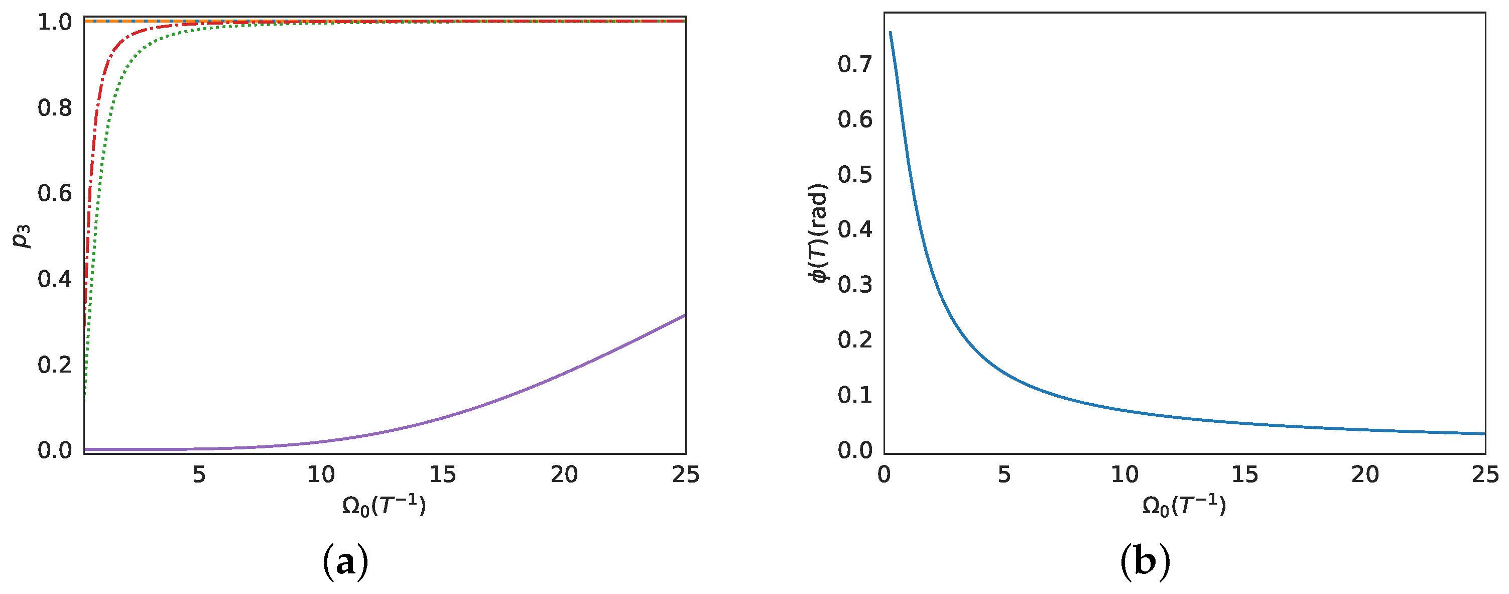
In Figure 3a, we plot the final population $p_3\left(T\right)$ versus parameter ${\mathsf{\Omega }}_0$ (in units of $T^{-1}$), in the absence of noise and for the various shortcuts considered so far: those derived from polynomial $\theta \left(t\right)$ with constant (blue solid line) and ramp (orange dashed line) $\mathsf{\Omega }\left(t\right)$ and the shortcut derived from Gaussian pulses (green dotted line). We also plot the efficiency of the simple STIRAP method with the Gaussian pulses of Equation (22) (solid purple line), which obviously lies well below that of the shortcuts, indicating that STIRAP requires substantially longer times or larger amplitudes in order to achieve comparable efficiency levels. Observe that both the shortcuts with constant $\mathsf{\Omega }\left(t\right)={\mathsf{\Omega }}_0$ and ramp $\mathsf{\Omega }\left(t\right)={\mathsf{\Omega }}_{0}t/T$ achieve perfect population transfer to level $|3\rangle$ even for very small values of ${\mathsf{\Omega }}_0$. This is not surprising since the corresponding controls ${\tilde{\mathsf{\Omega }}}_p,{\tilde{\mathsf{\Omega }}}_s$ contain the terms $4{\dot{\theta }}^2,2\dot{\varphi }$, respectively, which do not vanish as ${\mathsf{\Omega }}_0\to 0$. This is clearly demonstrated in Figure 4, where we display the controls and the evolution of populations for the shortcut with constant $\mathsf{\Omega }\left(t\right)={\mathsf{\Omega }}_0=0.1T^{-1}$. On the other hand, the shortcut derived from Gaussian pulses has a decreasing efficiency with decreasing ${\mathsf{\Omega }}_0$. For this shortcut, the variables $\theta ,\dot{\theta },\ddot{\theta }$ are independent of ${\mathsf{\Omega }}_0$ and depend only on parameters $\tau ,\sigma$; see Equation (23), which have been selected such that the corresponding boundary conditions in Equation (20) are satisfied with high precision. What actually fails for decreasing ${\mathsf{\Omega }}_0$ is the boundary condition $\varphi \left(T\right)=0$, as displayed in Figure 3b. In Figure 5a,b, we plot the controls and corresponding populations obtained for this shortcut when the small value ${\mathsf{\Omega }}_0=0.5T^{-1}$ is used. Observe that the performance (value of $p_3$) degrades when the Stokes pulse ${\tilde{\mathsf{\Omega }}}_s\left(t\right)$ acquires negative values. If we truncate the negative final part of the Stokes pulse, a better transfer can be achieved, as demonstrated in Figure 5c,d. The efficiency of this modified shortcut versus ${\mathsf{\Omega }}_0$ is also displayed in Figure 3a (red dashed-dotted line).

In the following section, we evaluate the performance of the presented STIRAP shortcuts in the presence of Ornstein–Uhlenbeck noise in the energy levels of the system.

3. Performance of the Shortcuts in the Presence of Ornstein–Uhlenbeck Noise in the Level Energies

We consider the system evolution under the total Hamiltonian:

$$H\left(t\right)=\tilde{H}\left(t\right)+H_n\left(t\right),$$

(24)

where $\tilde{H}\left(t\right)$ is given in Equation (18) and the noise term is:

$$H_n\left(t\right)=\frac{\hslash }{2}\left(\begin{array}{ccc}{n}_1\left(t\right)& 0& 0\\ 0& n_2\left(t\right)& 0\\ 0& 0& n_3\left(t\right)\end{array}\right),$$

(25)

with $n_i\left(t\right),i=1,2,3$, being independent Ornstein–Uhlenbeck noise processes. They are defined through the relations [33]:

$${\dot{n}}_i=-\frac{1}{{\tau }_c}{n}_i+\frac{1}{{\tau }_c}{w}_i,$$

(26)

where $w_i\left(t\right),i=1,2,3$, are independent Gaussian white noises with zero mean and correlations:

$$\langle w_i\left(t\right)w_j(t+\tau )\rangle =2{\sigma }_n^2{\tau }_c{\delta }_{ij}\delta \left(\tau \right).$$

(27)

The resulting Ornstein–Uhlenbeck processes are also zero mean Gaussian with correlations:

$$R_{n_i{n}_j}\left(\tau \right)=\langle n_i\left(t\right)n_j(t+\tau )\rangle ={\sigma }_n^2{\delta }_{ij}{e}^{-|\tau |/{\tau }_c}$$

(28)

and steady state probability distributions:

$$P_i\left(n\right)=\frac{1}{\sqrt{2\pi {\sigma }_n^2}}{e}^{-\frac{n^2}{2{\sigma }_n^2}}.$$

(29)

Obviously, parameter ${\tau }_c$ is the noise correlation time. For each process, the power spectral density is:

$$S_{n_i{n}_i}\left(\omega \right)={\int }_{-\infty }^{\infty }{R}_{n_i{n}_i}\left(\tau \right)e^{-i\omega \tau }d\tau =\frac{2{\sigma }_n^2{\tau }_c}{1+{\left(\omega {\tau }_c\right)}^2}$$

(30)

and the expectation value of the total power is:

$$\langle n_i^2\left(t\right)\rangle =R_{n_i{n}_i}\left(0\right)=\frac{1}{2\pi }{\int }_{-\infty }^{\infty }{S}_{n_i{n}_i}\left(\omega \right)d\omega ={\sigma }_n^2.$$

(31)

In the following simulations, the Ornstein–Uhlenbeck processes were implemented using the algorithm described in [33]. We used a fixed standard deviation ${\sigma }_n$, corresponding to fixed noise power, and various correlation times ${\tau }_c$. From Equation (30), corresponding to a low-pass filter with cut-off frequency ${\omega }_c=1/{\tau }_c$, it is obvious that for larger correlation times, the fixed noise power was distributed to lower frequencies $\omega$. Thus, for larger ${\tau }_c$, the noises in the energy levels were low frequency signals, which brought the system out of resonance for larger time intervals, leading to a degraded performance. Note that the noise model considered here, with independent noises of equal strength in each energy level, applies directly to the physical system of molecules in a liquid; see [32]. In atomic systems, usually the second level is more noisy than the others. Obviously, the first model with independent noises present in all levels provided a harder test for the efficiency of STIRAP shortcuts, and for this reason, we used it here.

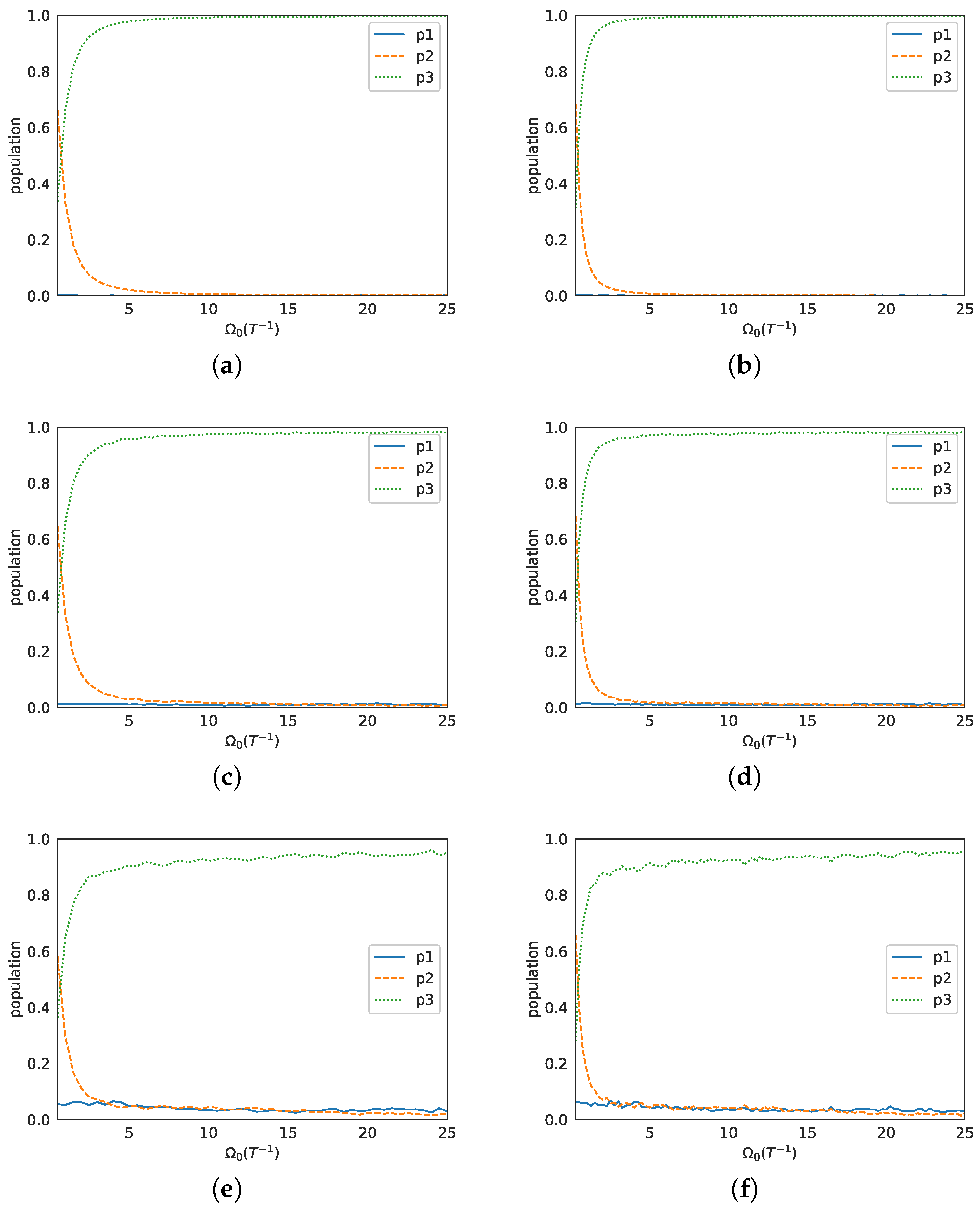
In Figure 6, we plot the final populations $p_i\left(T\right)={|{\tilde{c}}_1\left(T\right)|}^2,i=1,2,3$, versus parameter ${\mathsf{\Omega }}_0$ (in units $T^{-1}$) for the shortcuts derived from polynomial $\theta \left(t\right)$, with constant $\mathsf{\Omega }\left(t\right)={\mathsf{\Omega }}_0$ (first column) and ramp $\mathsf{\Omega }\left(t\right)={\mathsf{\Omega }}_{0}t/T$ (second column), in the presence of the aforementioned noise processes in the energy levels. We fixed ${\sigma }_n=5T^{-1}$ and used three different values of the correlation time, ${\tau }_c/T=0.008,0.08,0.8$, corresponding to each of the three rows from top to bottom. The diagrams were produced by averaging over the results of 200 simulations. Observe that for both shortcuts, the efficiency $p_3\left(T\right)$ had a similar robust behavior to this kind of noise, which was degraded as the noise correlation time increased.

In Figure 7, we display similar results for the two shortcuts derived from Gaussian pulses, with the first column corresponding to the usual shortcut and the second column to the modified one obtained by truncating the negative part of the Stokes pulse, while the three rows correspond to different noise correlation times. Observe that the behavior of these shortcuts was more robust than in the previous case. As before, the performance was degraded with increasing correlation time, but here, the reduction was milder. Note that the modified shortcut behaved better for smaller values of ${\mathsf{\Omega }}_0$, while for larger values, the two shortcuts had the same efficiency. The reason was that for larger ${\mathsf{\Omega }}_0$, the truncated negative part of the Stokes pulse became smaller, and the two shortcuts actually coincided.

Note that, since the two shortcut types used in Figure 6 and Figure 7 had different time dependence, the same value of parameter ${\mathsf{\Omega }}_0$ may correspond to different areas of the pump and Stokes pulses. In order to make a more fair comparison between them, we used two different ${\mathsf{\Omega }}_0$ resulting in similar pulse areas for the two shortcuts. Specifically, for the shortcut with constant $\mathsf{\Omega }\left(t\right)={\mathsf{\Omega }}_0$, we used the value ${\mathsf{\Omega }}_0=15T^{-1}$, while for the standard shortcut derived from Gaussian pulses, we used ${\mathsf{\Omega }}_0=10\pi T^{-1}$. The corresponding pulses are displayed in Figure 1a and Figure 2a, respectively. The areas of the pump and Stokes pulses were 11.34, 10.52 in the first case and 10.36, 12.36 in the second case, i.e., they had similar values. In Figure 8, we plot the time evolution of populations $p_i\left(t\right),i=1,2,3$, in the interval $0\le t\le T$. The first column shows results for the pulses of Figure 1a, while the second column for the pulses of Figure 2a. As before, the three rows correspond to different values of correlation time, ${\tau }_c/T=0.008,0.08,0.8$, while we set ${\sigma }_n=5T^{-1}$. Observe that for all cases, the shortcut derived from Gaussian pulses (second column) was more robust to noise than the shortcut derived from polynomial $\theta \left(t\right)$ with constant $\mathsf{\Omega }\left(t\right)={\mathsf{\Omega }}_0$ (first column). This difference became more pronounced for larger correlation times. A possible explanation of this behavior might be the observation that for the shortcut with constant $\mathsf{\Omega }\left(t\right)={\mathsf{\Omega }}_0$ (first column), the major changes in the populations took place during longer time intervals than the corresponding changes for the shortcut derived from Gaussian pulses (second column). Consequently, the evolution of populations in the first case was probably affected more by the low frequency noise corresponding to increasing correlation time ${\tau }_c$.

This observation can be further exploited to provide a rough explanation about the somehow strange dependence of efficiency versus ${\mathsf{\Omega }}_0$, for the shortcut with constant $\mathsf{\Omega }\left(t\right)={\mathsf{\Omega }}_0$ and noise correlation ${\tau }_c=0.8T$, displayed in Figure 6e. Observe that the efficiency $p_3\left(T\right)$ (green dotted line) initially dropped with increasing ${\mathsf{\Omega }}_0$, but then rose again, as ${\mathsf{\Omega }}_0$ increased further. In order to explain this behavior along the lines of the observation at the end of the previous paragraph, we needed an estimate of the duration during which the major changes in populations took place for a specific ${\mathsf{\Omega }}_0$. A rough such estimate was provided by the time $T_{0.9}$, needed so the population of level $|3\rangle$ rose from $p_3\left(t_1\right)=0.01$ to $p_3(t_1+T_{0.9})=0.9$, for the shortcut under consideration and in the absence of noise. In Figure 9, we plot the quantity $1-T_{0.9}/T$ as a function of ${\mathsf{\Omega }}_0$. Note the similarity with the efficiency $p_3\left(T\right)$ in Figure 6e. In closing, it is worth mentioning that a similar behavior to that displayed in Figure 6 was observed in [24] for assisted adiabatic passage, when there was exponentially correlated noise in the phases of the applied laser fields.

4. Conclusions

We studied the performance of two shortcuts to adiabaticity for the STIRAP system, in the presence of dephasing by exponentially correlated noise. For the first shortcut the mixing angle was a polynomial function of time, while the second shortcut was derived from Gaussian pulses. From numerical simulations, we found that both shortcuts performed quite well and robustly even in the presence of relatively large noise amplitudes, while their efficiency was degraded when the noise correlation time increased. With similar pulse amplitudes and durations, the efficiency of classical STIRAP was highly degraded even in the absence of noise. We also found that, when using pulses with similar areas for the two STIRAP shortcuts, the shortcut derived from Gaussian pulses appeared to perform better. The current work is expected to have a wide range of applications, since STIRAP plays an important role in the implementation of many modern quantum technologies.

References

1. Bergmann, K.; Theuer, H.; Shore, B.W. Coherent population transfer among quantum states of atoms and molecules. Rev. Mod. Phys. 1998, 70, 1003. [Google Scholar] [CrossRef]
2. Král, P.; Thanopulos, I.; Shapiro, M. Coherently controlled adiabatic passage. Rev. Mod. Phys. 2007, 79, 53. [Google Scholar] [CrossRef] [Green Version]
3. Vitanov, N.V.; Rangelov, A.A.; Shore, B.W.; Bergmann, K. Stimulated Raman adiabatic passage in physics, chemistry, and beyond. Rev. Mod. Phys. 2017, 89, 015006. [Google Scholar] [CrossRef]
4. Bergmann, K.; Nägerl, H.C.; Panda, C.; Gabrielse, G.; Miloglyadov, E.; Quack, M.; Seyfang, G.; Wichmann, G.; Ospelkaus, S.; Kuhn, A.; et al. Roadmap on STIRAP applications. J. Phys. B At. Mol. Opt. Phys. 2019, 52, 202001. [Google Scholar] [CrossRef] [Green Version]
5. Kobrak, M.N.; Rice, S.A. Selective photochemistry via adiabatic passage: An extension of stimulated Raman adiabatic passage for degenerate final states. Phys. Rev. A 1998, 57, 2885. [Google Scholar] [CrossRef]
6. Dreisow, F.; Szameit, A.; Keil, M.H.M.R.; Nolte, S.; Tünnermann, A.; Longhi, S. Adiabatic transfer of light via a continuum in optical waveguides. Opt. Lett. 2009, 34, 2405. [Google Scholar] [CrossRef]
7. Menchon-Enrich, R.; Benseny, A.; Ahufinger, V.; Greentree, A.D.; Busch, T.; Mompart, J. Spatial adiabatic passage: A review of recent progress. Rep. Prog. Phys. 2016, 79, 074401. [Google Scholar] [CrossRef] [PubMed] [Green Version]
8. Golter, D.A.; Wang, H.L. Optically driven Rabi oscillations and adiabatic passage of single electron spins in diamond. Phys. Rev. Lett. 2014, 112, 116403. [Google Scholar] [CrossRef] [PubMed]
9. Kumar, K.S.; Danilin, A.V.A.S.; Paraoanu, G.S. Stimulated Raman adiabatic passage in a three-level superconducting circuit. Nat. Commun. 2016, 7, 10628. [Google Scholar] [CrossRef] [Green Version]
10. Guéry-Odelin, D.; Ruschhaupt, A.; Kiely, A.; Torrontegui, E.; Martínez-Garaot, S.; Muga, J.G. Shortcuts to adiabaticity: Concepts, methods, and applications. Rev. Mod. Phys. 2019, 91, 045001. [Google Scholar] [CrossRef]
11. Unanyan, R.G.; Yatsenko, L.P.; Bergmann, K.; Shore, B.W. Laser-induced adiabatic atomic reorientation with control of diabatic losses. Opt. Commun. 1997, 139, 48. [Google Scholar] [CrossRef]
12. Demirplak, M.; Rice, S.A. Adiabatic population transfer with control fields. J. Phys. Chem. A 2003, 107, 9937. [Google Scholar] [CrossRef]
13. Berry, M.V. Transitionless quantum driving. J. Phys. A Math. Theor. 2009, 42, 365303. [Google Scholar] [CrossRef] [Green Version]
14. Motzoi, F.; Gambetta, J.M.; Rebentrost, P.; Wilhelm, F.K. Simple pulses for elimination of leakage in weakly nonlinear qubits. Phys. Rev. Lett. 2009, 103, 110501. [Google Scholar] [CrossRef] [PubMed] [Green Version]
15. Chen, X.; Ruschhaupt, A.; Schmidt, S.; del Campo, A.; Guéry-Odelin, D.; Muga, J.G. Fast optimal frictionless atom cooling in harmonic traps: Shortcut to adiabaticity. Phys. Rev. Lett. 2010, 104, 063002. [Google Scholar] [CrossRef] [PubMed]
16. Masuda, S.; Nakamura, K. Fast-forward of adiabatic dynamics in quantum mechanics. Proc. R. Soc. A 2010, 466, 1135. [Google Scholar] [CrossRef]
17. Deffner, S.; Jarzynski, C.; del Campo, A. Classical and quantum shortcuts to adiabaticity for scale-invariant driving. Phys. Rev. X 2014, 4, 021013. [Google Scholar] [CrossRef] [Green Version]
18. Claeys, P.W.; Pandey, M.; Sels, D.; Polkovnikov, A. Floquet-engineering counterdiabatic protocols in quantum many-body systems. Phys. Rev. Lett. 2019, 123, 090602. [Google Scholar] [CrossRef] [Green Version]
19. Li, Y.; Chen, X. Shortcut to adiabatic population transfer in quantum three-level systems: Effective two-level problems and feasible counterdiabatic driving. Phys. Rev. A 2016, 94, 063411. [Google Scholar] [CrossRef] [Green Version]
20. Baksic, A.; Ribeiro, H.; Clerk, A.A. Speeding up adiabatic quantum state transfer by using dressed states. Phys. Rev. Lett. 2016, 116, 230503. [Google Scholar] [CrossRef] [Green Version]
21. Du, Y.-X.; Liang, Z.; Li, Y.; Yue, X.; Lv, Q.; Huang, W.; Chen, X.; Yan, H.; Zhu, S. Experimental realization of stimulated Raman shortcut-to-adiabatic passage with cold atoms. Nat. Commun. 2016, 7, 12479. [Google Scholar] [CrossRef] [PubMed]
22. Zhou, B.B.; Baksic, A.; Ribeiro, H.; Yale, C.G.; Heremans, F.J.; Jerger, P.C.; Auer, A.; Burkard, G.; Clerk, A.A.; Awschalom, D.D. Accelerated quantum control using superadiabatic dynamics in a solid-state lambda system. Nat. Phys. 2017, 13, 330. [Google Scholar] [CrossRef] [Green Version]
23. Mortensen, H.L.; Sørensen, J.J.; Mølmer, K.; Sherson, J.F. Fast state transfer in a Λ-system: A shortcut-to-adiabaticity approach to robust and resource optimized control. New J. Phys. 2018, 20, 025009. [Google Scholar] [CrossRef]
24. Demirplak, M.; Rice, S.A. Assisted adiabatic passage revisited. J. Phys. Chem. B 2005, 109, 6838. [Google Scholar] [CrossRef]
25. Chen, X.; Lizuain, I.; Ruschhaupt, A.; Guéry-Odelin, D.; Muga, J.G. Shortcut to adiabatic passage in two- and three-level atoms. Phys. Rev. Lett. 2010, 105, 123003. [Google Scholar] [CrossRef]
26. Giannelli, L.; Arimondo, E. Three-level superadiabatic quantum driving. Phys. Rev. A 2014, 89, 033419. [Google Scholar] [CrossRef] [Green Version]
27. Torosov, B.T.; Valle, G.D.; Longhi, S. Non-Hermitian shortcut to stimulated Raman adiabatic passage. Phys. Rev. A 2014, 89, 063412. [Google Scholar] [CrossRef] [Green Version]
28. Masuda, S.; Rice, S.A. Fast-forward assisted STIRAP. J. Phys. Chem. A 2015, 119, 3479. [Google Scholar] [CrossRef] [Green Version]
29. Masuda, S.; Rice, S.A. A model study of assisted adiabatic transfer of population in the presence of collisional dephasing. J. Chem. Phys. 2015, 142, 244303. [Google Scholar] [CrossRef]
30. Danilin, A.V.A.S.; Paraoanu, G.S. Superadiabatic population transfer in a three-level superconducting circuit. Science Adv. 2019, 5, eaau5999. [Google Scholar]
31. Impens, F.; Guéry-Odelin, D. Fast quantum control in dissipative systems using dissipationless solutions. Sci. Rep. 2019, 9, 4048. [Google Scholar] [CrossRef] [PubMed] [Green Version]
32. Demirplak, M.; Rice, S.A. Optical control of molecular dynamics in a liquid. J. Chem. Phys. 2002, 116, 8028. [Google Scholar] [CrossRef]
33. Fox, R.F.; Gatland, I.R.; Roy, R.; Vemuri, G. Fast, accurate algorithm for numerical simulation of exponentially correlated colored noise. Phys. Rev. A 1988, 38, 5938. [Google Scholar] [CrossRef] [PubMed] [Green Version]
34. Shi, Q.; Geva, E. Stimulated Raman adiabatic passage in the presence of dephasing. J. Chem. Phys. 2003, 119, 11773. [Google Scholar] [CrossRef]
35. Zeng, Y.X.; Gebremariam, T.; Ding, M.S.; Li, C. The influence of non-Markovian characters on quantum adiabatic evolution. Ann. Phys. 2019, 531, 1800234. [Google Scholar] [CrossRef] [Green Version]
36. Falci, G.; Cognata, A.L.; Berritta, M.; D’Arrigo, A.; Paladino, E.; Spagnolo, B. Design of a Lambda system for population transfer in superconducting nanocircuits. Phys. Rev. B 2013, 87, 214515. [Google Scholar] [CrossRef]
37. Stefano, P.G.D.; Paladino, E.; Pope, T.J.; Falci, G. Coherent manipulation of noise-protected superconducting artificial atoms in the Lambda scheme. Phys. Rev. A 2016, 93, 051801(R). [Google Scholar] [CrossRef] [Green Version]
38. Issoufa, Y.H.; Messikh, A. Effect of dephasing on superadiabatic three-level quantum driving. Phys. Rev. A 2014, 90, 055402. [Google Scholar] [CrossRef]
39. Boyers, E.; Pandey, M.; Campbell, D.K.; Polkovnikov, A.; Sels, D.; Sushkov, A.O. Floquet-engineered quantum state manipulation in a noisy qubit. Phys. Rev. A 2019, 100, 012341. [Google Scholar] [CrossRef] [Green Version]
40. Ibáñez, S.I.; Chen, X.; Torrontegui, E.; Muga, J.G.; Ruschhaupt, A. Multiple Schrödinger pictures and dynamics in shortcuts to adiabaticity. Phys. Rev. Lett. 2012, 109, 100403. [Google Scholar] [CrossRef] [Green Version]
41. Lu, X.; Ruschhaupt, A.; Muga, J.G. Fast shuttling of a particle under weak spring-constant noise of the moving trap. Phys. Rev. A 2018, 97, 053402. [Google Scholar] [CrossRef] [Green Version]
Figure 1. (a) Pump and Stokes pulses (in units T 1 ) for the shortcut to adiabaticity where the mixing angle is a polynomial function of time and Ω ( t ) = Ω 0 is a constant. (b) Corresponding time evolution of the level populations. (c,d) Controls (in units T 1 ) and populations for the case where Ω ( t ) = Ω 0 t / T is a ramp. In both cases, the value Ω 0 = 15 T 1 is used.
Applsci 10 01580 g001
Figure 2. (a) Pump and Stokes pulses (in units T 1 ) for the shortcut to adiabaticity derived from Gaussian pulses. (b) Corresponding evolution of populations. Gaussian parameters: Ω 0 = 10 π T 1 , τ = T / 8 , and σ = T / 6 .
Applsci 10 01580 g002
Figure 3. (a) The efficiency (final population p 3 ( T ) of level | 3 ) of the various shortcuts to diabaticity versus parameter Ω 0 , in the absence of noise. The shortcuts derived from polynomial θ ( t ) with constant (blue solid line) and ramp (orange dashed line) Ω ( t ) have a unit efficiency independent of Ω 0 , while the efficiency of the shortcut derived from Gaussian pulses (green dotted line) and its modification (red dashed-dotted line) increases gradually to unity with increasing Ω 0 . We also plot for reference the efficiency of the simple STIRAP method with Gaussian pulses (22) (purple solid line). (b) Final angle ϕ ( T ) versus Ω 0 for the shortcut derived from Gaussian pulses. Obviously, the boundary condition ϕ ( T ) = 0 is severely violated for smaller Ω 0 .
Applsci 10 01580 g003
Figure 4. (a) Controls (in units T 1 ) and (b) time evolution of populations for the shortcut to adiabaticity derived from polynomial θ ( t ) with constant Ω ( t ) = Ω 0 = 0.1 T 1 .
Applsci 10 01580 g004
Figure 5. (a) Pump and Stokes pulses (in units T 1 ) for the shortcut derived from Gaussian pulses with Ω 0 = 0.5 T 1 . (b) Corresponding time evolution of the level populations. (c,d) Controls (in units T 1 ) and populations for the modified shortcut where the final negative part of the Stokes pulse is truncated.
Applsci 10 01580 g005
Figure 6. Final populations p i ( T ) , i = 1 , 2 , 3 , as functions of parameter Ω 0 , for the STIRAP shortcuts derived from polynomial θ ( t ) with (a,c,e) constant Ω ( t ) = Ω 0 and (b,d,f) ramp Ω ( t ) = Ω 0 t / T . The three rows correspond to three different values of the noise correlation time, τ c / T = 0.008 , 0.08 , 0.8 , respectively, while the standard deviation is set to σ n = 5 T 1 . For the cases corresponding to τ c / T = 0.8 (last row), where the averages still fluctuate, we also display the 98% confidence intervals.
Applsci 10 01580 g006
Figure 7. Final populations p i ( T ) , i = 1 , 2 , 3 , as functions of parameter Ω 0 , for the STIRAP shortcuts derived from Gaussian pulses. In (a,c,e) standard shortcut has been used and in (b,d,f) the modified shortcut has been used. The three rows correspond to three different values of the noise correlation time, τ c / T = 0.008 , 0.08 , 0.8 , respectively, while the standard deviation is set to σ n = 5 T 1 .
Applsci 10 01580 g007
Figure 8. Evolution of populations in the interval 0 t T for the shortcut pulses displayed in Figure 1a (first column), Figure 2a (second column), and different values of the noise correlation time: (a,b) τ c / T = 0.008 , (c,d) τ c / T = 0.08 , and (e,f) τ c / T = 0.8 . These results are obtained after averaging over many simulation instances. The trajectories do not exhibit a high-frequency “noisy” behavior, since the power of the considered noise processes is concentrated in lower frequencies, affecting only the final efficiency.
Applsci 10 01580 g008
Figure 9. Quantity 1 T 0.9 / T versus Ω 0 , where T 0.9 is the time needed so the population of level | 3 rises from p 3 ( t 1 ) = 0.01 to p 3 ( t 1 + T 0.9 ) = 0.9 , for the shortcut with constant Ω ( t ) = Ω 0 and in the absence of noise.
Applsci 10 01580 g009