1. Introduction
Vacuum-assisted composite fabrication processes are widely used for producing large components with good quality, and widely applied in many industries due to being low cost, time-consuming, simplicity of the required equipment and better ecology conditions at the manufacturing. The technical details and components of the vacuum infusion in composite manufacturing are described in many papers, technical reports, dissertations [
1,
2,
3,
4,
5] and others.
The history of the vacuum infusion process in the production of composites should be dated back to 1945, when two engineers at Marco Chemical, Inc. Muscat and Plainfield proposed a new method of molding, patented by them in 1950 [
3]. Despite the extremely great attention of specialists and scientists, which was manifested in the large number of patents and publications issued, in the development of its various kinds [
6], the wide industrial use of the process is constrained by its lack of reliability in terms of quality assurance and the absence of irreparable defects, especially in the manufacture of the critical load-carrying composite structures.
Meanwhile, some modifications of the VARTM (Vacuum-Assisted Resin Transfer Molding) processes have been developed to improve its quality, versatility and performance that allowed to significantly expand the scope of the process in the practice of composites manufacturing. Among the developed contrivances, which were able to overcome the difficulties associated with low permeability of the preforms, are a high permeability (HPM) and flow distribution media [
7,
8], air-permeable membrane [
7], use of multiple injection lines and vents with independent control of resin and vacuum pressure [
2,
7,
9,
10,
11,
12,
13,
14]. A distributed thermal control sometimes is used.
Due to the above-mentioned improvements while ensuring a low degree of the resin cure at the end of the preform filling [
13,
15,
16,
17,
18,
19,
20,
21] they were successfully implemented in the manufacture of aircraft structures (usually shell type) [
1,
22,
23], blades of the wind turbines [
1,
20,
24,
25,
26,
27], ship’s hulls [
1,
2,
20,
24,
25], details of spacecraft [
1,
28], large-sized parts of cars bodies [
29,
30] and in the defense industry [
7,
27].
Despite the abundance of completed and increasing number of ongoing studies of the processes, in each case, the developer must solve a number of difficult problems due to the features of vacuum infusion. The most important feature of VARTM is due to the presence of a flexible vacuum bag that covers the upper surface of the infused preform. This causes the compressive effect of atmospheric pressure on the preform, and the result of this action is its compression deformation, which changes according to the location of advancing front of the resin. In the dry region, where the low air pressure
is supplied due to connection to the vacuum vent, the compressive pressure exerting a compression effect on the preform is equal to
, whereas in the region filled with liquid resin, the pressure approaching the atmospheric pressure counteracts the external, atmospheric pressure
[
6]. This phenomenon, which significantly changes the permeability of the preform for the moving liquid resin, can contribute to the creation of incompletely saturated zones and dry spots [
7,
12,
24,
28,
30,
31]. Another reason for the preform compaction is a wetting compaction, which can arise due to the lubricant effect of the resin when it wets the fibers [
32]. This compaction accompanies the moving front of the resin, further worsening the conditions of its propagation, and also causes the hysteresis behavior of the preform when it is unloaded from external pressure.
The presence of differently oriented layers in laminated preform leads to the fact that the impregnation of the layers depends on their permeability in the direction of the resin front propagation, as well as leads to the layers deformation that disrupts their packing [
5,
16].
During infusion of large-sized thin-walled aircraft structures, the resin can transform from a liquid to a gel state, without having time to fill the entire preform due to the long path [
2,
10,
23,
33]. This fact makes it necessary to thoroughly analyze the thermal-kinetic and rheological state of the resin during the infusion process.
A change in the compressing state along the porous preform and the resin rheology during the process can cause difficulty in ensuring the uniformity of the product’s thickness and the homogenous distribution of the reinforcing and resin fractions [
8,
34,
35].
The solution of the listed problems using the trial and error method requires considerable time, financial expenses due to the high cost of the components, raising the importance of the development of process modeling tools that allow taking into account with maximum accessible precision the following process features:
Geometry of preform and mold;
Their mechanical and thermal properties, which determine the effect of pressures and temperatures on the spread of liquid resin in a medium with varying porosity and permeability;
The evolution of the thermal-kinetic and rheological properties of the resin;
A process scheme including numbers, locations and shapes of the liquid resin gates and vacuum vents. Such a modeling system would make it possible to reconstruct the nature of the motion of the resin front and its state throughout the entire technological cycle, to select the optimal process parameters to ensure the production of defect-free products. Historically, the first such system was the LIMS software [
3,
9,
12,
36], the theoretical foundations of which were presented in the 1990s of the 20th century and presented in [
37]. Lately, a kind of similar systems have been developed and used by some scientists: PAM-RTM [
9,
13,
15,
38]; RTM-WORKS [
2,
24,
26]; 3DINFIL [
39]; RTMSim [
40]; Moldex3D RTM [
41] and the ANSYS Fluent module [
23,
25,
32]. All of these systems are based on the use of the so-called finite element/control volume (FE/CV) method, which uses special means of monitoring the front movement of the resin to eliminate the need to work with the moving boundaries and the deformed FE mesh. Some features of the FE/CV method are presented here to justify the proposed approach.
In the fundamental work [
36], the modeling approach that was used to describe the resin flow process is based on the FE/CV method. The modeled part’s geometry was assumed as shell-like, the thickness of which is much smaller than other dimensions. This approach was implemented in almost all later works [
10,
25,
27,
38], including the most recent ones [
5,
16,
20].
The FE/CV method proposed in [
36] and used in all subsequent works does not require the rebuilding of the mesh as the resin front moves in areas with complex geometries. A key feature of the FE/CV method is a rough approximation of the shape of the modeled region, combined with careful consideration of mass conservation. Three basic steps are needed to simulate an FE/CV flow [
37]: (1) use the FE solution to obtain the pressure distribution in the area filled with resin; (2) calculate the resin flow rate; and (3) trace the front of the resin flow. The commonly used approach to construct control volumes introduces an error when using skewed elements, which is almost always observed in the case of complex part geometry. For such cells, the mass conservation condition may be violated. In some works, a modification of the method is proposed, according to which the finite elements and control volumes coincide.
Tracking the interface between air and resin is the main goal of our study. In [
10,
13,
25,
27,
37,
38], which use the FE/CV approach, the tracking was implemented by solving the continuity equation for the volume fraction of resin
Vr. The construction of the resin flow theory in these works always begins with Darcy’s law, which determines the dependence of the superficial resin velocity on the pressure gradient in the liquid phase, on the porous media permeability tensor and the resin viscosity. Some works, for example [
42], use Brinkman’s correction to Darcy’s law to take into account the pressure drop due to shear stresses at the interface liquid—porous region.
Heat transfer and thermal-kinetic processes affecting the resin rheology have been studied in a number of works [
6,
13,
19,
20,
21,
43,
44,
45] to reduce the filling time of the preform and eliminate the dry spots. The influence of process parameters, in particular heating rates and holding times, on the resin viscosity and laminate infiltration was evaluated during experimental tests and confirmed by monitoring the process.
There are also a number of works (e.g., [
3,
36]) focused on the construction of analytical models of infusion processes. Despite the relative simplicity and impossibility of using analytical approaches for modeling the real structures, they can be used to test more complex models on simple systems, as well as in experimental evaluations of the properties of preforms and resins.
The work [
46] presents the lumped model of VARTM with parameters, developed using the mechanical-electrical analogy. This model was intended to describe the flow of fluid through preform’s macropores and the absorption of resin by micropores in fiber bundles. To characterize the double fiber reinforcement, two physical phenomena are used, described in the work by lumped elements: resistance to the flow of liquid resin and the effect of its absorption during infusion.
In some works, the problem of process optimization is considered by which, in the broad sense, we mean the determination of the values of controlled parameters (design variables) that ensure the achievement of the best results (objectives). Optimization approaches and technologies can be divided into the following four kinds.
The first kind of optimization problem includes the classical investigations of the process output at varying controlled parameters (inputs) using some experimental methods. The paper [
28] reports about a microscopic study of the void content at the locations near the inlet as well as near the outlet of the infused preform at the varying independently controlled resin gates and vacuum vents pressures. A minimum filling time and absence of the dry spots were accepted as objectives in the experimental work [
6], where design variables were: parameters of the temperature cure cycle (heating rate at the first and second ramps, temperatures and durations during dwell sections).
The second kind is based on the numerous computer simulations and their results’ analysis to choose better process conditions. Dong [
9,
10] optimizes the filling time of preform and tries to eliminate the dry spots by varying the resin gate and vacuum vent diameters, their numbers and locations using FE/CV-based software. Influence of the heating rates and isothermal holds on the uniformity of the temperature and degree of cure fields during resin impregnation were studied in [
21] using the FE software ABAQUS. In order to provide a resin flowing profile uniformity and make the infusion time less than resin gel time, the authors of [
2,
24] used RTM-Worx software to optimize the manufacturing process of the boat hulls by manual changing injection gate position, length and spacing of minor pipes for parallel and fish-bone arrangements of the pipes.
The third kind combines the methodology of the two previous ones: computer simulation and experiment, the results of which are used to set parameters and validate the model of the infusion process. In the paper [
38], Zhao with co-workers informs about the minimization of the filling time in grooved foam sandwich composites changing the resin sources pattern at the experiments and numerical simulations. In article [
41], a flow front control system was developed using a real-time assessment of the permeability/porosity ratio on the base information obtained by the visualization system monitored the porous panel infusion. This approach substantially used the metamodel of the radial basis function (RBF), obtained as a result of training by Moldex 3D simulation module. The responses of this artificial neural network are used to predict the position of the front of the future flow by entering the injection pressure, the current position of the flow front and the calculated permeability/porosity ratio. By carrying out optimization based on a metamodel, the injection pressure value is obtained, which must be implemented at each stage.
The most advanced fully functional optimization systems belonging to the fourth kind include a process simulation module (forward problem solver) and optimizer, which carries out the multiple calls of the forward problem according to some optimization strategy, and forms the optimum solutions set in the objective space. The structure, organization and logic of the prototype of such optimization systems are described with the necessary completeness in an innovative work [
37], which uses the FE/CV modeling method, and the results of such a system were published in [
12]. The most important part of this paper is aimed at the problem of the dry spots’ formation, detection and evolution during infusion. It considers in detail conditions and evidence of dry spots formation at its surrounding by the inner and outer flow fronts. On the base of the numerous fulfilled simulations, the authors formulate the very useful recommendations that can be used in a practice. The dry spot detection algorithm, which is explained in [
12], requires significant computational efforts, therefore it is not very efficient, especially for the parts of complex 3D geometry. Moreover, the proposed technique includes the rebuilding of FE mesh in the vicinity of the flow front to supply the necessary accuracy of its configuration [
37].
Concluding our analysis of the considered works, it should be noted that the most important problem of the dry spots formation in the infusible preform was not solved with the necessary accuracy and reliability, which is due to the difficulties in reconstructing the movement of the resin front. The reason for this is the extremely high computational complexity of solving the problem of the resin dynamics in a porous medium at moving boundaries, as well as the insufficient accuracy of the widely used FE/CV method, which makes strict requirements for the design of cells of a control volume. Therefore, the main purpose of the present work is the development of a system for diagnosing and reliably predicting the occurrence of incompletely saturated and dry places at the VARTM. This system should provide the reconstruction of the motion of the resin front in preforms of complex 3D geometry, identification of the dry spot formation and effectively simulate the resin infusion dynamics to work as the forward problem solver that will be repeatedly called by the optimization module.
This paper is organized as follows. First, we present some results of two experimental studies with large Carbon Fiber Reinforced Plastic (CFRP) panels during vacuum infusion, where resin front advancement and dry spots formation were monitored in time. The next part contains the problem statement where we formulate the resin infusion model as the coupled two-phase (air/resin) media dynamics problem, where the phase field equation is accepted as the ruling one. In order to simplify the verification of the new modeling approach, we neglect the heat transfer, the thermal-kinetics, the wetting compaction and the change of the part’s dimension effects during filling and post-filling stages. On the base of the problem statement, we present its computer implementation in the FE Comsol Multiphysics 5.2 a (COMSOL AB, Stockholm, Sweden) software environment and describe the model’s structure and function, specially intended to identify the time instants and location of dry spots forming during simulation. Finally, we present some simulation results and consider how to use the model together with the optimization module, as well as the abilities of the developed MATLAB R2016 a (MathWorks Inc., Natick, MA, USA) module, destined to determine the evolution of dry spots formed by analyzing the postprocessing of the FE solution.
2. Vacuum Infusion of Large CFRP Parts: Experiment
In order to understand how the dry spots are formed during resin front advances in the porous preform, the experimental vacuum infusion processes for two different CFRP panels were carried out. At the manufacturing of both panels, the carbon fiber fabric CC245 with weaving twill 4/4, mass density 240 g/m2 and thickness 0.28 mm +/− 15% was used. To speed up the filling, Gerster HPM tape was laid in accordance with the selected method. A semi-permeable membrane VAP3D-C2003 was used to effectively remove air while retaining resin in a preform. The infused epoxy compound SR1710 with hardener SD8822 (Sicomin) had viscosity ~0.1 Pa·s at 25 °C. The air dissolved in resin was evacuated before the start of the process in the special vessel Vacmobiles RT 19/11 where low air pressure was supplied by the vacuum station Vacmobiles 20/2 (Vacmobiles Lim., Auckland, New Zealand).
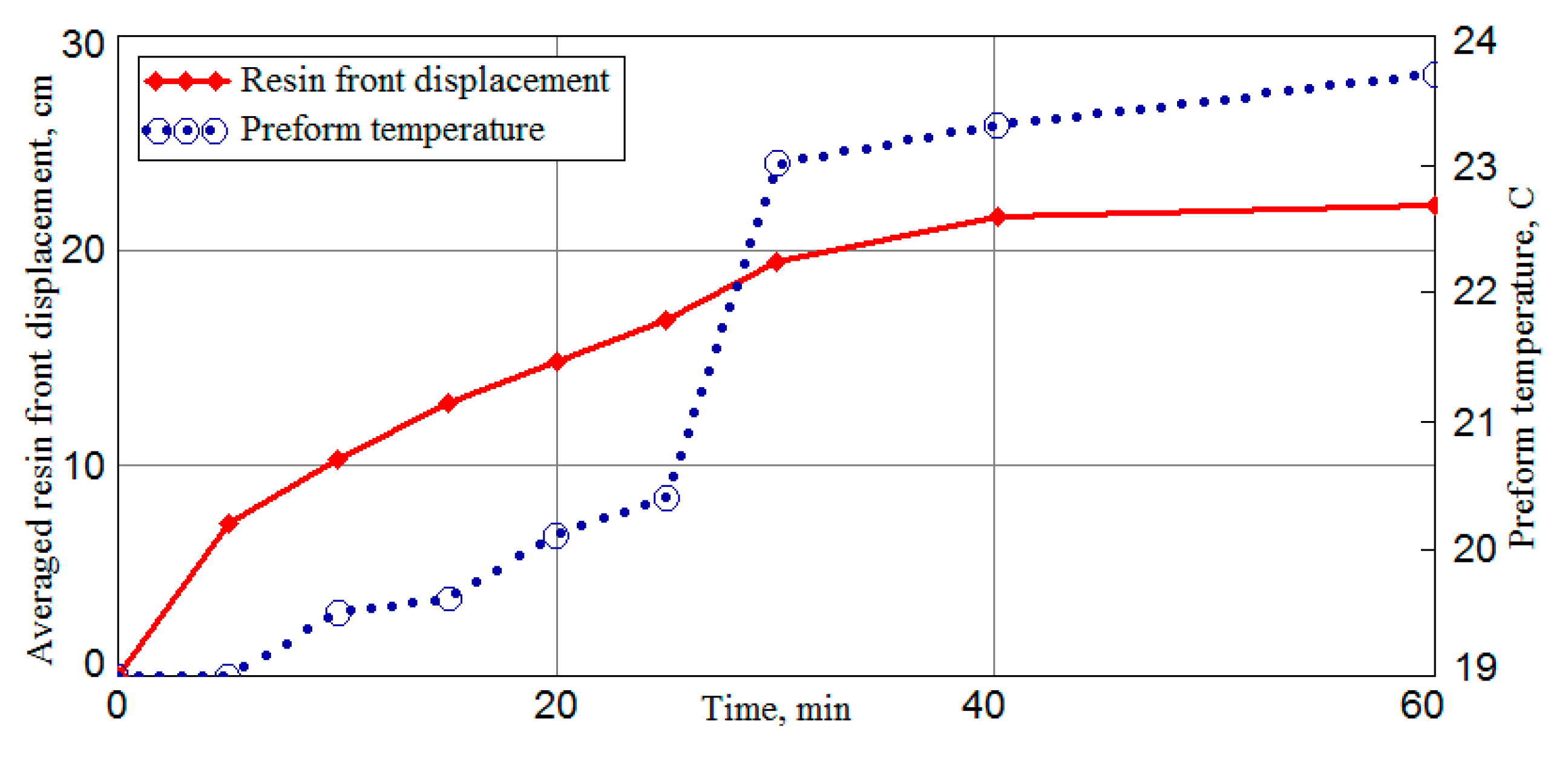
The first thin-walled rectangular panel of dimensions (800 × 700) mm with thickness 1.5 mm was an 8 layered cross-ply symmetric balanced laminate. Laying of HPM, hoses for pumping out the vacuum and resin injection was carried out along three sides around the perimeter of the panel. The vacuum infusion process was carried out at the ambient temperature 19 °C; the averaged preform temperature in the filled region and resin front position recorded every 5 min (see
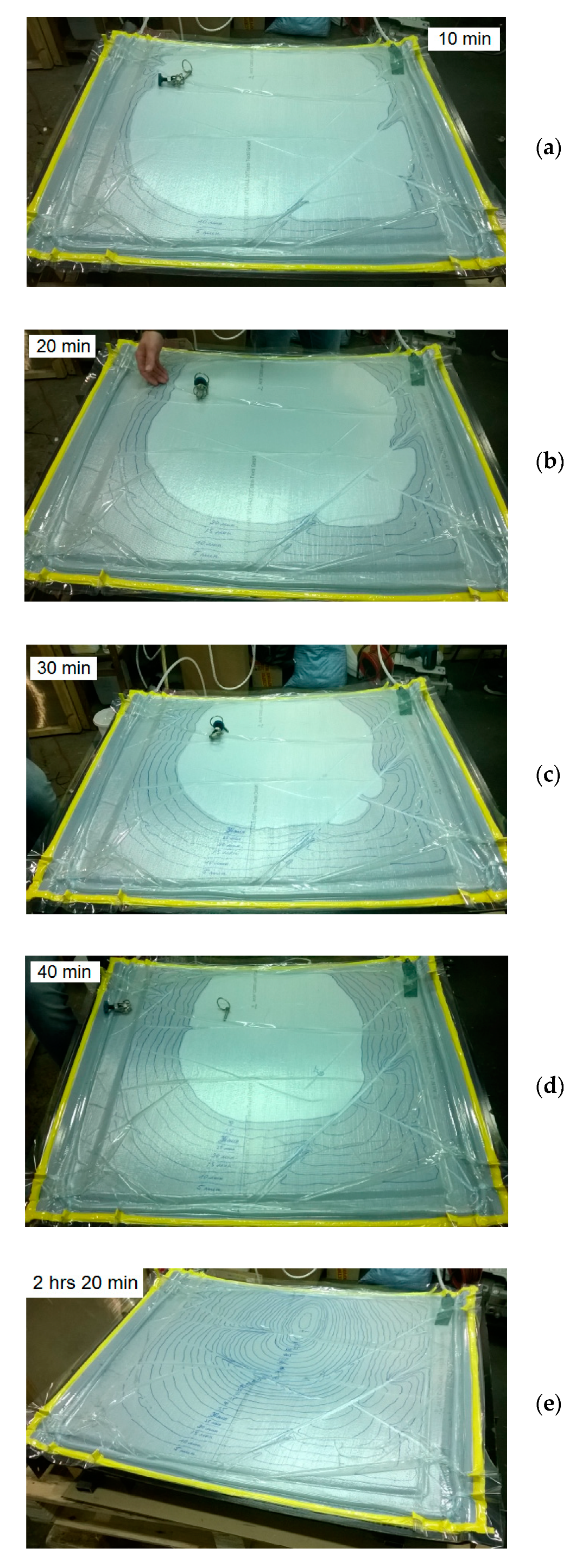
Figure 1). The dynamics of the preform resin infusion is illustrated by a series of photographs in
Figure 2.
The propagation speed of the resin front began to decline sharply after 40 min from the start of the process. Obviously, this is caused in part by the polymerization reaction of the resin, accompanied by an increment in temperature (see
Figure 1), partly by the closure of the resin fronts encountered, as a result of which the conditions for the penetration of vacuum to the dry preform region surrounded by the resin worsened (see
Figure 2d). After 2 h and 20 min, the movement of the resin ceased. A gradual decrease in the front velocity in the time interval 0–40 min is in full agreement with the observations [
3,
8,
27,
35,
39,
40].
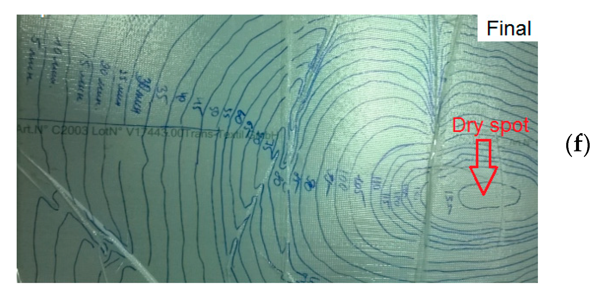
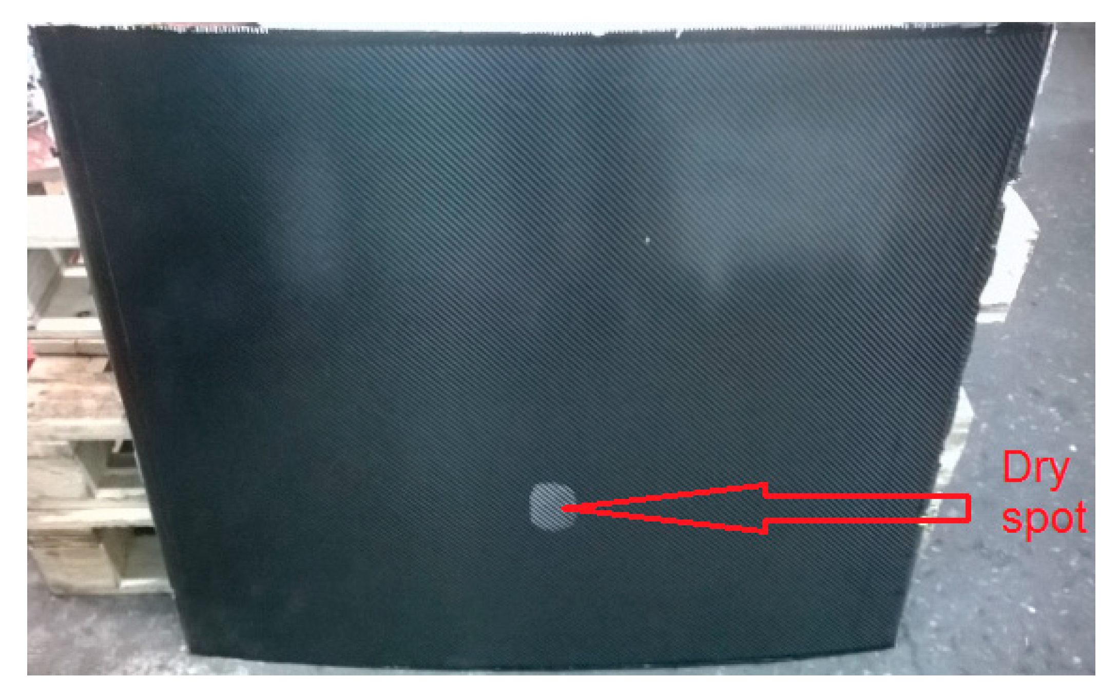
Photograph of the ready infused panel is shown in
Figure 3, where the formed dry spot is clearly visible. It arose as a result of the closure of the resin front, called in paper [
12] as the inner front, i.e., surrounding the void area with resin in the inner part of the preform.
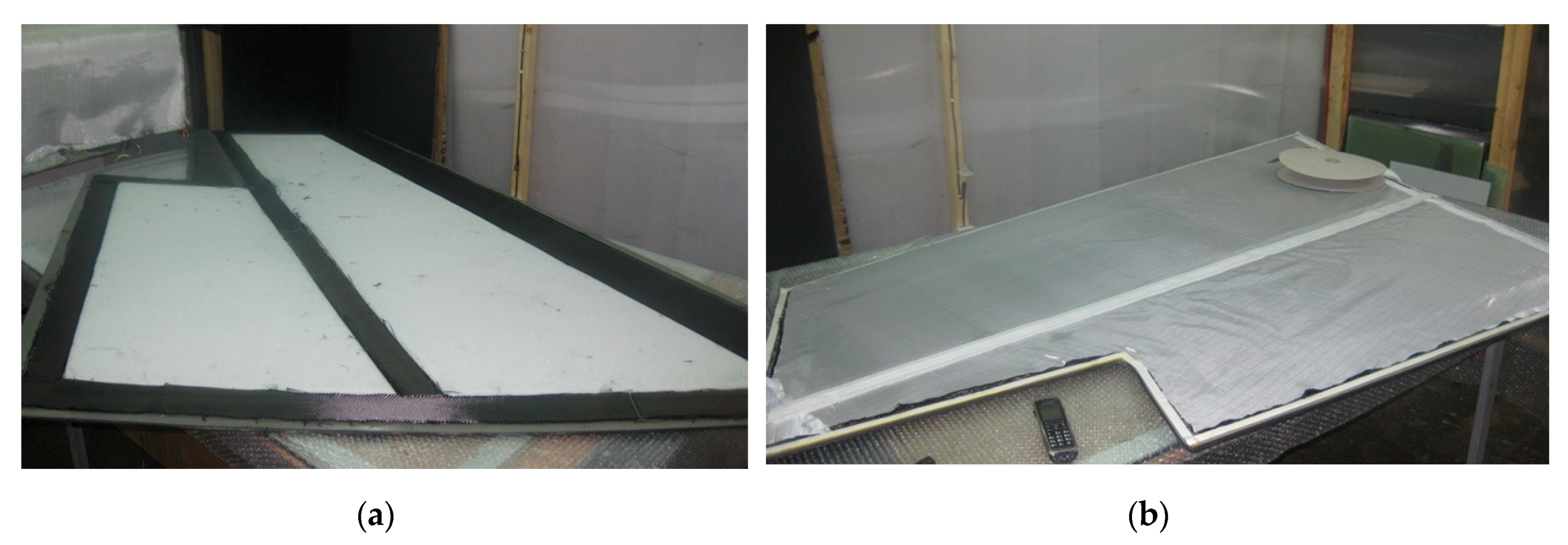
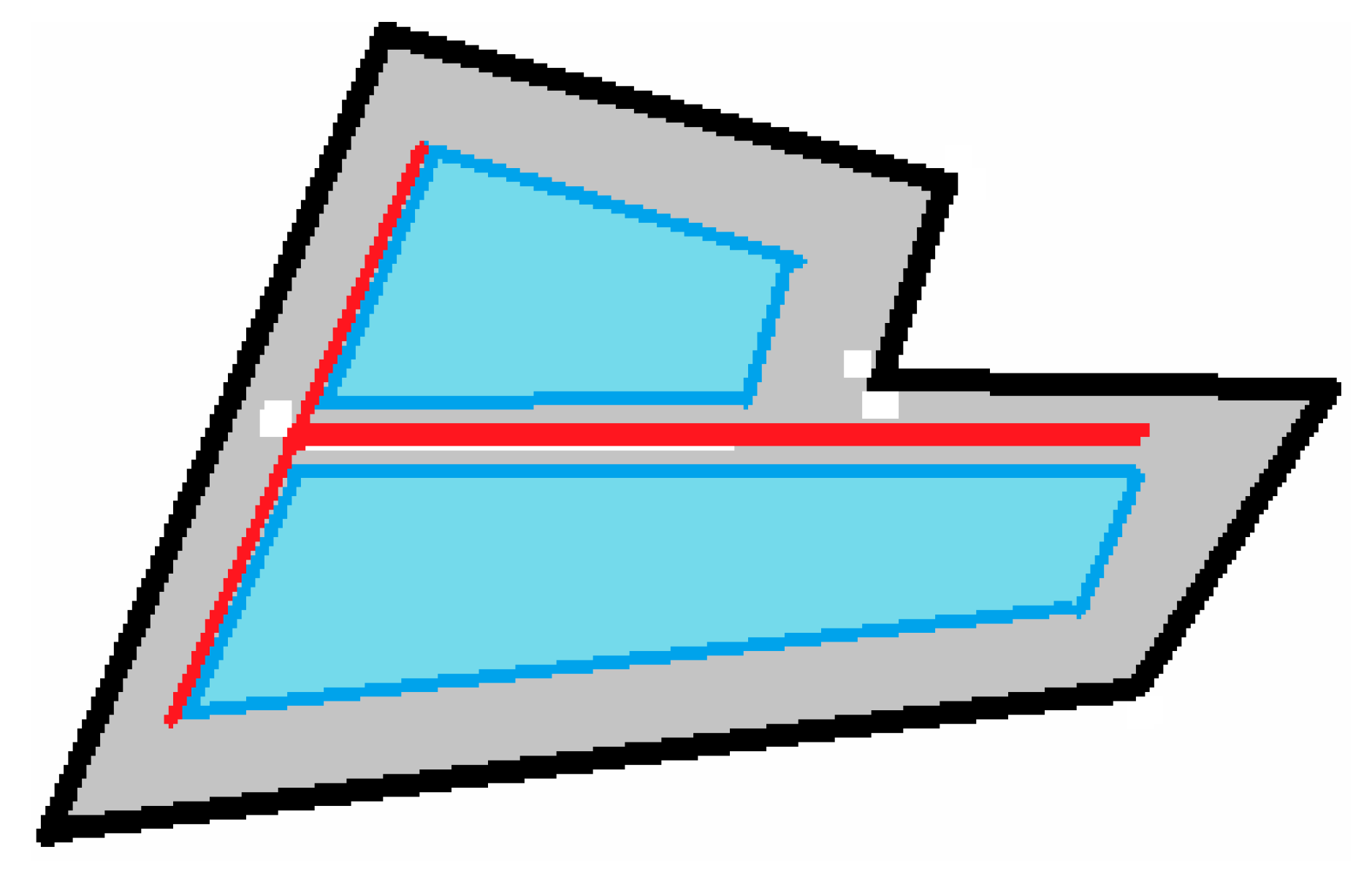
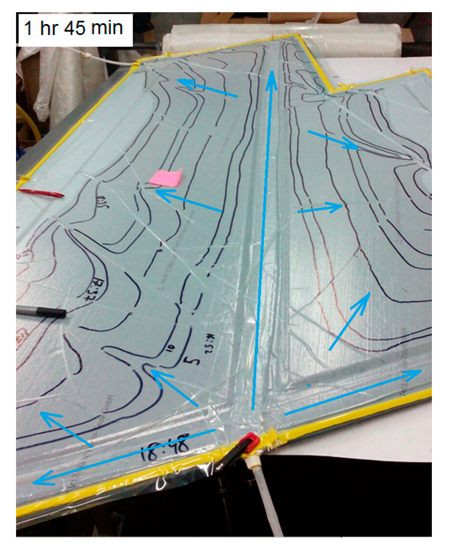
Much more difficult in terms of ensuring the quality of impregnation is the tail panel of a light aircraft with an overall size of more than 2 m. At the assembly of the technological packet, 4 layers of carbon fabric are laid sequentially over the entire area of the tooling, then foam plates (see
Figure 4a). The space between these foam plates is filled with carbon fabric ribbons (8 layers), and the whole sandwich is covered with 4 layers of carbon fabric, a semi-permeable membrane (see
Figure 4b) and a vacuum bag film that is sealed around the perimeter. The resin feed channel is shown in
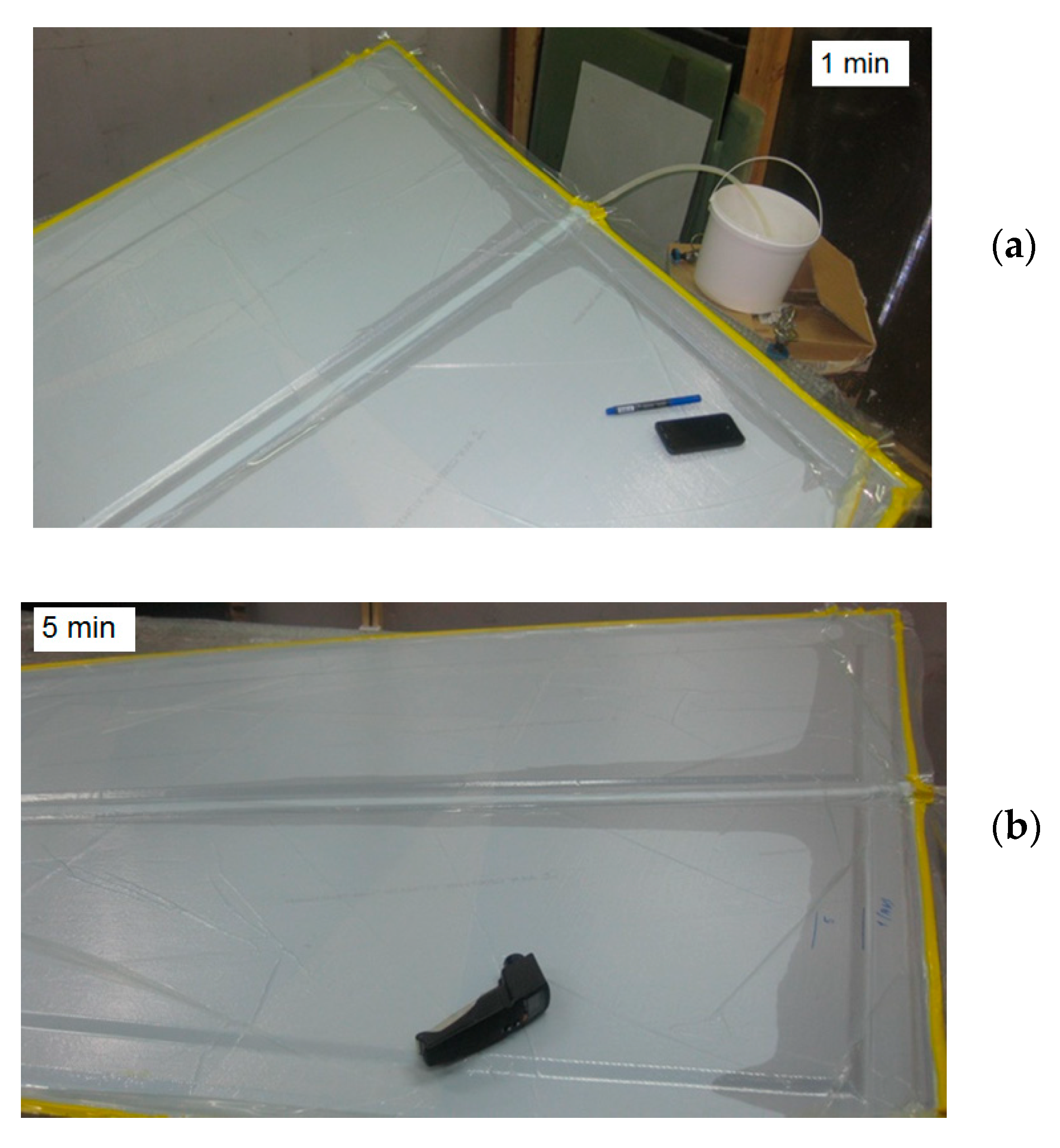
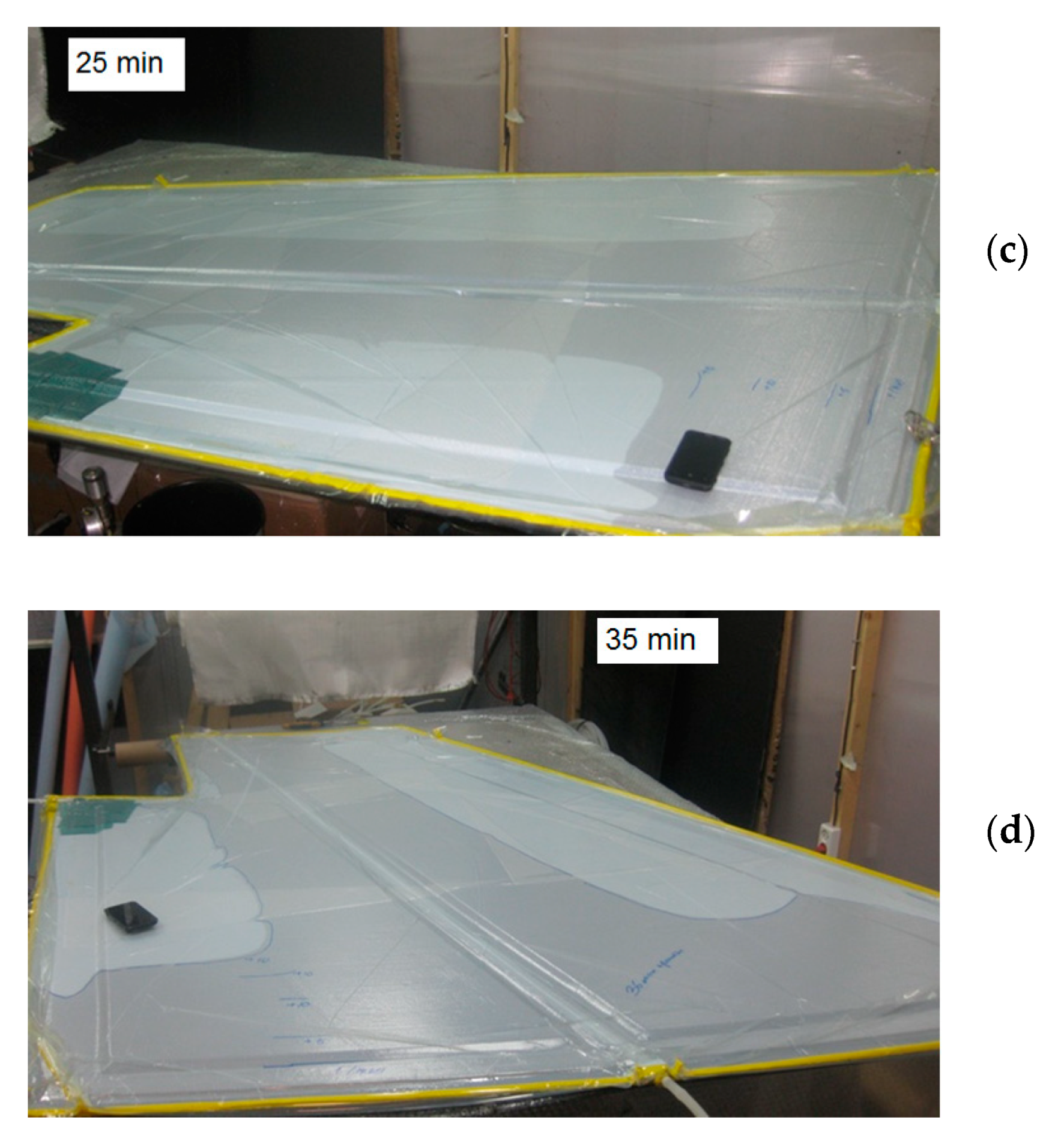
Figure 5 by red lines. The resin front propagation in time is present in
Figure 6, and its positions at the different time instants of the infusion process are shown together in
Figure 7.
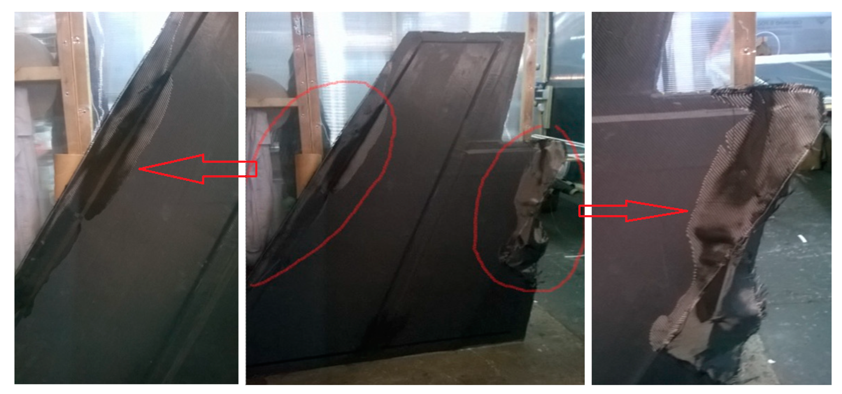
One can see in
Figure 7 that within 1 h and 45 min, the resin front did not reach the forward edge of the panel and the corner at its rear. This caused the fatal defect of the panel, which is shown in
Figure 8 after polymerization. The experiment showed the formation of dry spots as a result of stopping the outer front, as described in [
12].
The considered defects most often arise during the infusion of large-sized structures of complex geometry, when some parts of the convoluted front of the resin move toward each other or toward the boundary corners of the infusing structure forming closed loops. The cost of such tests by trial and error is very high. Thus, the ability of modeling systems replacing the trial and error method to correctly restore the front movement is the most important quality of such systems. The approach presented below is aimed specifically at achieving this ability in the system being created.
3. Model of the Resin Infusion: Problem Statement
The fundamental difference between the proposed approach and those considered above is the interdependence of the equations of the coupled problem, the solution of which describes the dynamics of liquid resin in a porous preform. The approaches discussed above used the Darcy’ equation as the leading (ruling) equation:
where
u is the superficial resin velocity, [
K] is the permeability tensor of the porous medium,
μ is the resin viscosity and
is the pressure gradient in the liquid phase. The proposed approach is based on the use as the leading equation, describing the motion of the interface between two contacting phases—the front of the moved resin. In this case, the calculation of the velocity field, depending on the pressure gradient in the liquid, will be made based on the result obtained when determining the shape and position of the front. To some extent, this approach repeats the methodology used in [
47], where a new numerical algorithm is proposed for modeling the dynamics of the interface between two immiscible phases. This interface is a thin layer, across which its physical properties change sharply, but continuously, and its evolution is determined by a phase field variable, which obeys the Cahn–Hilliard convection–diffusion-type equation. Its solution allows directly monitoring the interface and provides the correct interfacial tension due to the free energy accumulated in the separation layer. The phase field method does not require a regular FE mesh, a computational domain of simple form and spatial periodicity, which is required by other methods (e.g., the FE/CV method). This is important for modeling large-scale stream systems with complex and multiple interfaces, especially in three-dimensional (3D) cases.
Let the system includes two immiscible phases A and B. The phase field variable
ϕ is introduced so that the concentrations of components A (resin) and B (void, vacuum) are (1 +
ϕ)/2 and (1 −
ϕ)/2, respectively. Note that hereinafter everywhere, in order to avoid unacceptable confusion of quantities, the phase field variable will be denoted as
ϕ and preform porosity as
Vϕ. For the mixing energy, we take a form analogous to the form of the Lagrangian of the Ginzburg–Landau equation for the complex field of Cooper’s pairs:
where
λ is the mixing energy density with force dimension and
ε is the capillary width, which scales with the thickness of the diffuse interface. As
ε → 0, the ratio
λ/
ε gives the interfacial tension
σ in the classical sense:
The equation describing the evolution of a phase field variable is the Cahn–Hilliard equation [
48]:
where
G (Pa) is a chemical potential:
and
(m
3s/kg) is the phases mobility. Mobility
determines the time scale of the Cahn–Hilliard diffusion and should be large enough to maintain a constant interfacial thickness, but small enough so that the convective terms are not excessively damped. Mobility
is a function of the thickness of the interface according to
γ =
χε2, where
χ is the mobility setting parameter. The Cahn–Hilliard equation forces a value for
ϕ of 1 or −1, with the exception of a very thin region at the interface between two media.
The Comsol FE system, in which the simulation was performed, uses the splitting of the fourth-order Equation (4) into two second-order partial differential equations (PDE):
The local filling of the micro volumes of the preform
Vr can be expressed through the phase field variable
ϕ by the relation:
so that a completely filled volume (
) corresponds to a value
, an empty volume (
) corresponds to a value
.
The boundary conditions of the phase field equation are shown in
Table 1, while the used values of all equation’s parameters are present in
Table 2.
The initial condition for the variable ϕ defined everywhere in the volume of preform is .
The second equation of the coupled problem describing the dynamics of the viscous resin should be an equation connecting the field of the resin’s driving pressures with the velocity field of the medium. The Richards equation [
49] representing fluid motion in unsaturated soils is adopted as:
which models the behavior of saturation
S as a function of pressure
p, permeability and porosity
Vϕ. Permeability in Equation (9) is the product of constant permeability
K and relative permeability
. The saturation
S in Equation (9) is an analog of the filling, i.e., resin volume fraction
Vr.
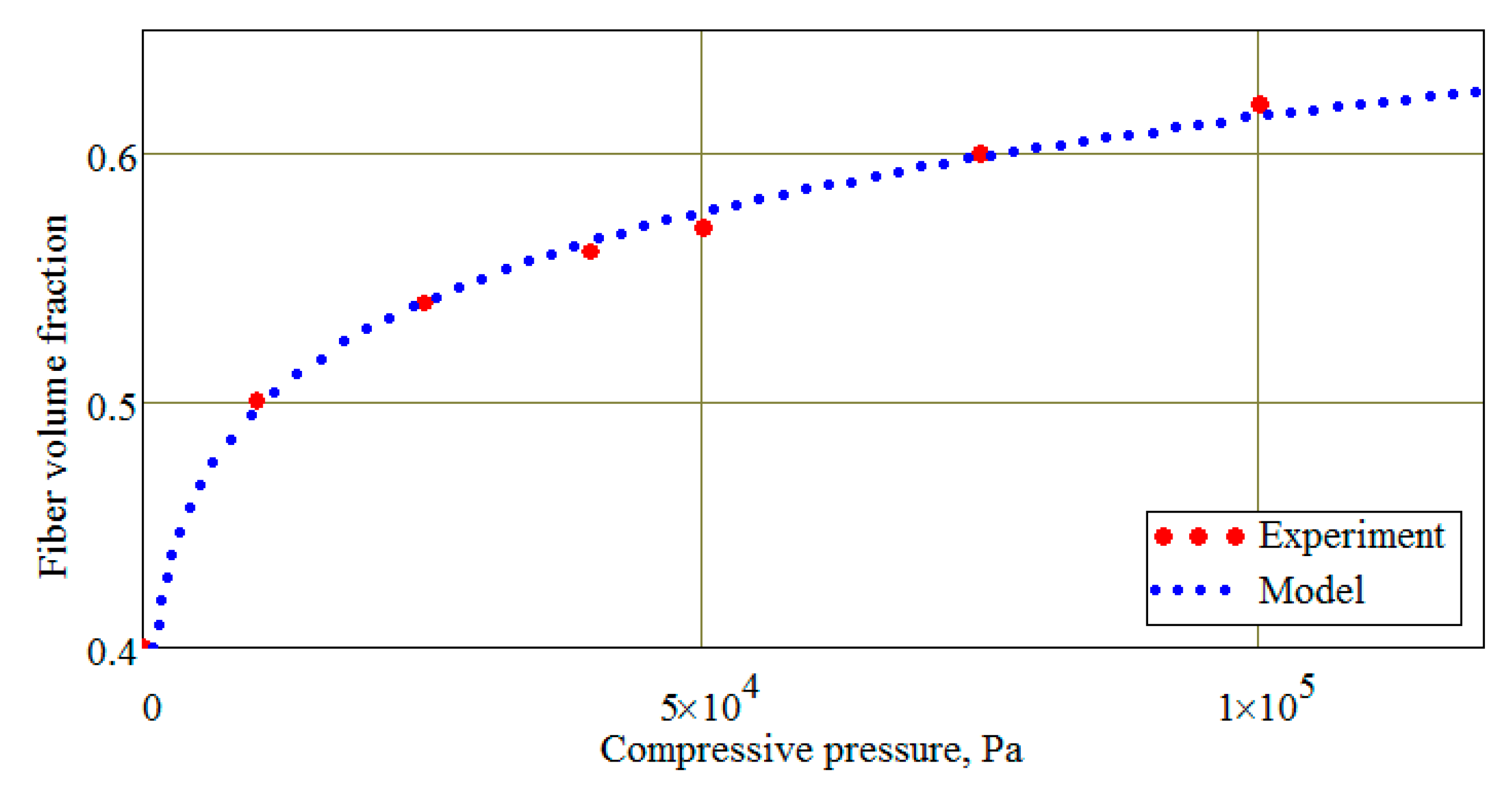
To correctly take into account the void preform’s compacting and the resulting change in its permeability at the vacuum infusion processes, the following models were most widely used [
6,
34]: compacting model—changes in the reinforcing volume fraction
Vf (see
Figure 9):
where the compacting pressure
Pcomp is the difference between atmospheric pressure and the pressure in the region inside the preform,
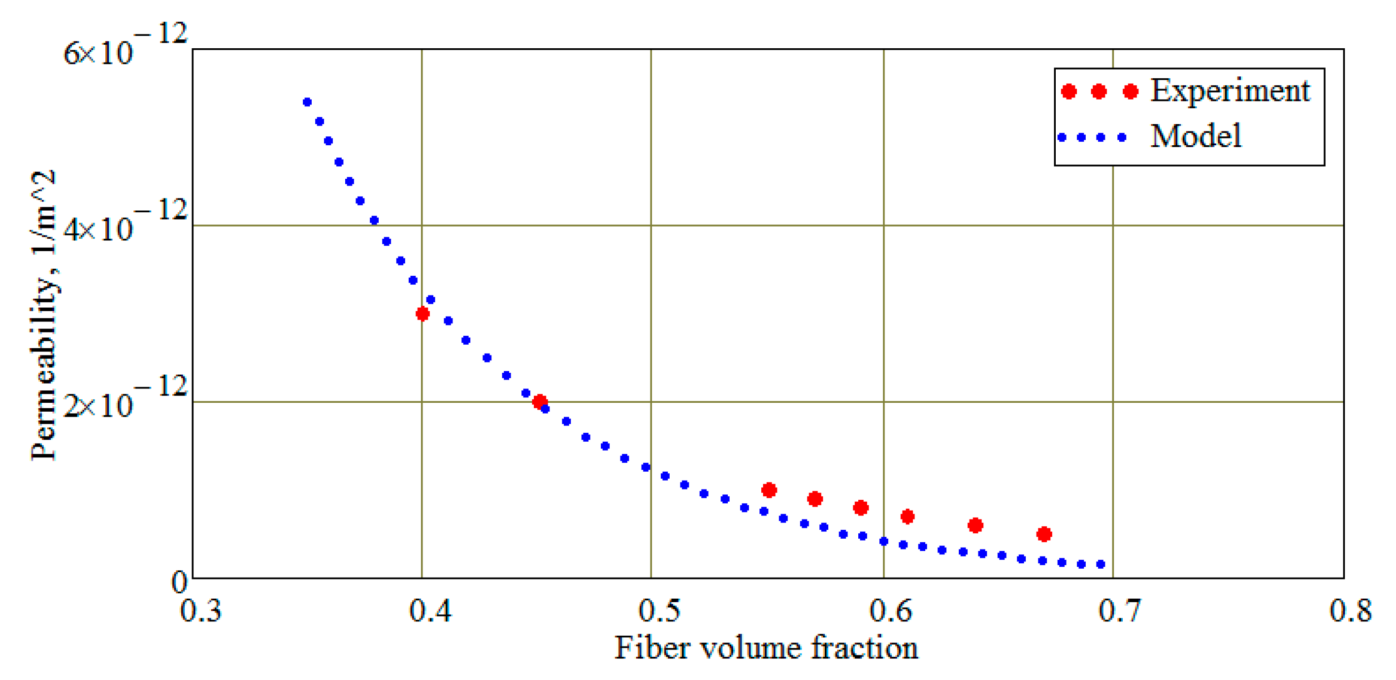
Vf0 is the reinforcing fiber volume fraction at the zero compacting pressure and the Kozeny–Karman model for the permeability
K of the porous medium:
where the Kozeny constant
k, determined experimentally, reflects the structure of the porous medium, i.e., depends on the geometry of the reinforcement. Combining Equations (10) and (11), it is easy to obtain the dependence of permeability on compacting pressure. Using the relation between porosity
Vϕ and
Vf, the dependence of permeability can also be expressed in terms of the porosity
These models have been used in our study; their graphical representations are present in
Figure 9 and
Figure 10 together with the experimental data used for these models’ identification.
In Equation (9), the value of the saturation can be expressed as some function of pressure that activates the movement of the liquid [
49]. In the work [
50], on the base of the results of van Genuchten’s research [
51], it was shown that the saturation dependence on the pressure can be satisfactorily described by the function:
where a variable
is determined experimentally, which was implemented in [
49]. Satisfactory agreement with the experimental data was achieved for the value
, where the reference pressure
is taken equal to the current atmospheric pressure. Thus, after performing time differentiation, Equation (9) is transformed to the form:
It supplements the phase field equation, is connected with it through porosity and allows us to establish a relationship between pressure and fluid flow rate using Relation (1) of Darcy’s law, which includes the pressure value determined from Equation (14). The pressure field in the preform, determined from Equation (14), is used to calculate the compacting pressure
acting externally on the porous structure of the preform
and, therefore, changing its porosity and fiber volume fraction according to Equation (10).
Equation (14) must be valid in the entire volume of the preform, both in filled and in empty areas. Consequently, the values of permeability and viscosity should vary in accordance with the resin filling
Vr and porosity
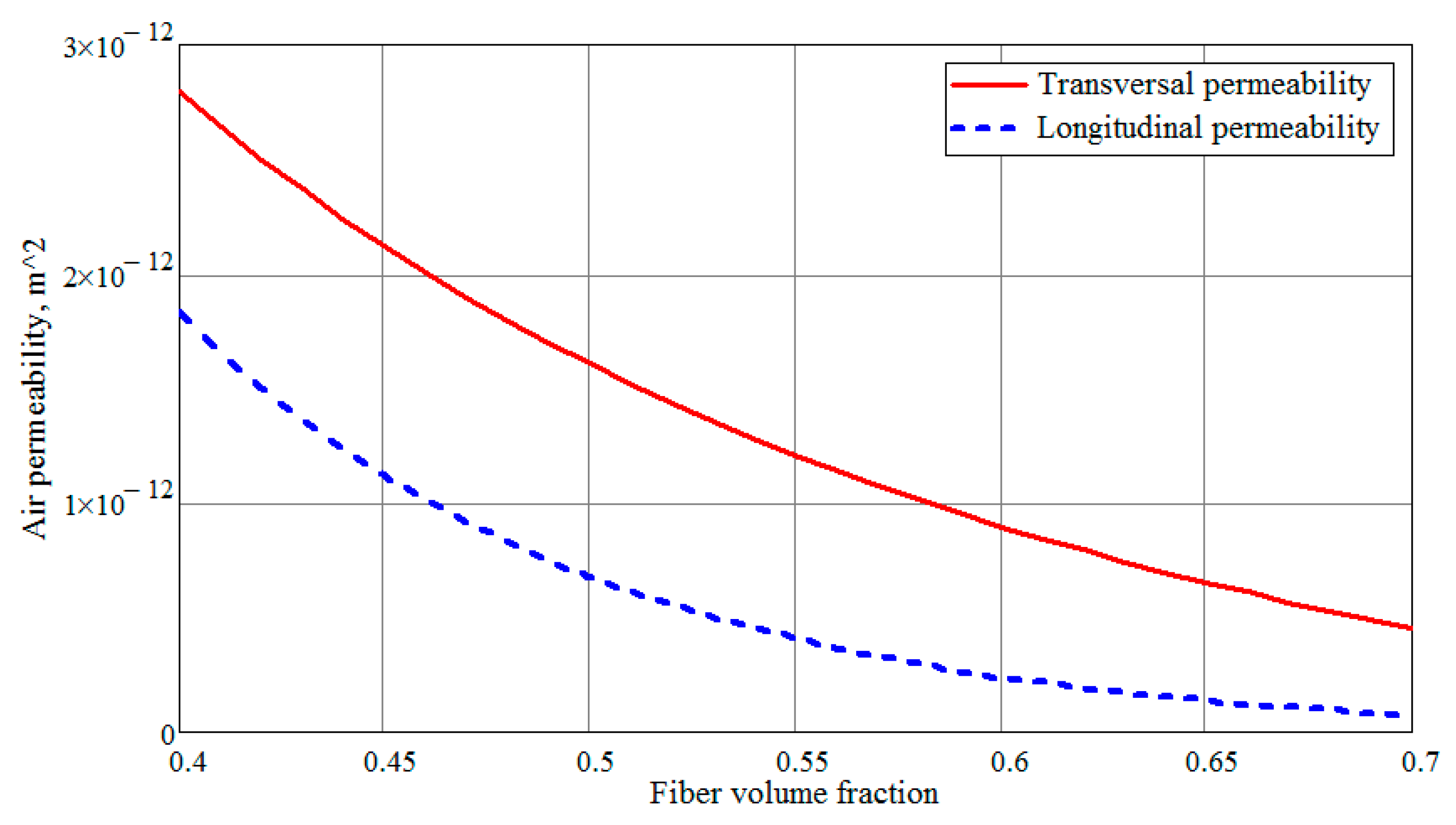
Vϕ. The resin permeability dependence on the fiber volume fraction is described by Equation (11). The study of the air permeability along and transverse of the hexagonally arranged fabrics with different fiber volume fractions suggest the following relations for these permeabilities [
52]
where these models parameters are:
,
,
and
μm is a fiber radius. The validity of the relations (16) is confirmed by numerous experimental data for different CFRP and GFRP (Glass Fiber Reinforced Plastic) fabrics, e.g., [
52,
53]. These dependencies are present in
Figure 11. A comparison of
Figure 10 and
Figure 11 demonstrates a very close coincidence of the nature of permeability for liquid and air; therefore, the dependence of permeability for both contacting phases is assumed to be the same, and it was calculated by the Formula (11).
However, the viscosities of the liquid resin and air differ several orders of magnitude. Since temperature effects are neglected at this stage of the study, the viscosity of the resin is assumed to be unchanged and equal to 0.1 Pa·s. The air pressure does not affect to the air viscosity in a wide pressure range, whereas its value increases according to quasi-linear law from
Pa·s up to
Pa·s in the temperature range (20°–300°) C [
54]. In the present study, the air viscosity is accepted as
Pa·s.
The boundary conditions of Equation (14) are present in the
Table 3.
The initial condition for the pressure specified everywhere in the preform’s volume is .
The system of equations above closes the formulation of the problem of 3D modeling the dynamics of liquid resin in a porous preform. Beyond the scope of this problem, there remains the issue of localization of dry spots-closed air “traps” observed experimentally (see
Figure 2 and
Figure 7). During the infusion process, several traps can form, but the formation of the first such trap indicates a violation of the manufactured structure’s quality. Hence, if the modeling module works under the control of the optimization module, the resulting solution may be discarded without further consideration, and calculations can be continued at the changed process design variables. When the module is operating in standalone mode, the simulation can continue to identify all critical time instants and other formed dry spots. To perform such an analysis, a MATLAB algorithm for the processing of simulation results has been developed. In such cases, the simulation continues until the blocking of the vacuum vent by the resin flow. An indicator of this blockage is a condition:
at the boundary Γ
out surrounding the vacuum port.
In order to identify time instant when a first dry spot arises and its localization, the use of change in averaged pressure in the non-filled zones of the prepreg has been proposed. The essence of the method is as follows. Let pressure in the vacuum vent varies rather slowly according to the sinusoidal law so that the period of these oscillations is, e.g., ~30 s:
where the mean value and amplitude of the pressure variation are accepted as
Pa and
Pa, respectively. The pressure in a void area connected to the vacuum vent must be uniform in every point of this area due to the insignificant air viscosity. As the resin front advances, some areas may become blocked from the one connected to the vacuum line. In this area, however, as well as in those connected with vacuum, resin fraction is very small, i.e.,
. However, as a result of blocking, this region remains under the pressure at which it was blocked, not under a sinusoidally changing one. As an indicator of the moment of a void trap closure, we introduce the expression:
where
is the Heaviside function, and
is the low resin filling, below which integration is performed. Formula (19) calculates at each simulation step the time-varying average value of pressure in all “low filled” areas, or, more precisely, in areas separated from the filled ones by the resin front. Until the first trap closes, approximate equality
will take place, signaling that the ratio between the mean pressure and the amplitude of its variation is almost unchanged. After the closure, the newly formed empty region is isolated from the vacuum line, and the pressure in it cannot vary according to Equation (18). Hence, the ratio
will be changed, which is easily recorded, and can serve as a trigger for stopping the simulation. The computational cost of the integration in Equation (18) is very small. In addition, after recording the moment of formation of a dry spot, the simulation can be stopped when searching for the best solution among a large number of them. Obviously, the sensitivity of the proposed indicator of the void trap formation will depend on the period of pressure oscillations, which, however, should be an order of magnitude greater than the time integration step.
The dry spots localization and their shape evolution can be studied by means of a special algorithm processing the simulation results. Its main functions and components will be presented in the example of simulated vacuum infusion, which was implemented at the different process conditions.
4. FE Simulation of the Vacuum Infusion Process: Results and their Analysis
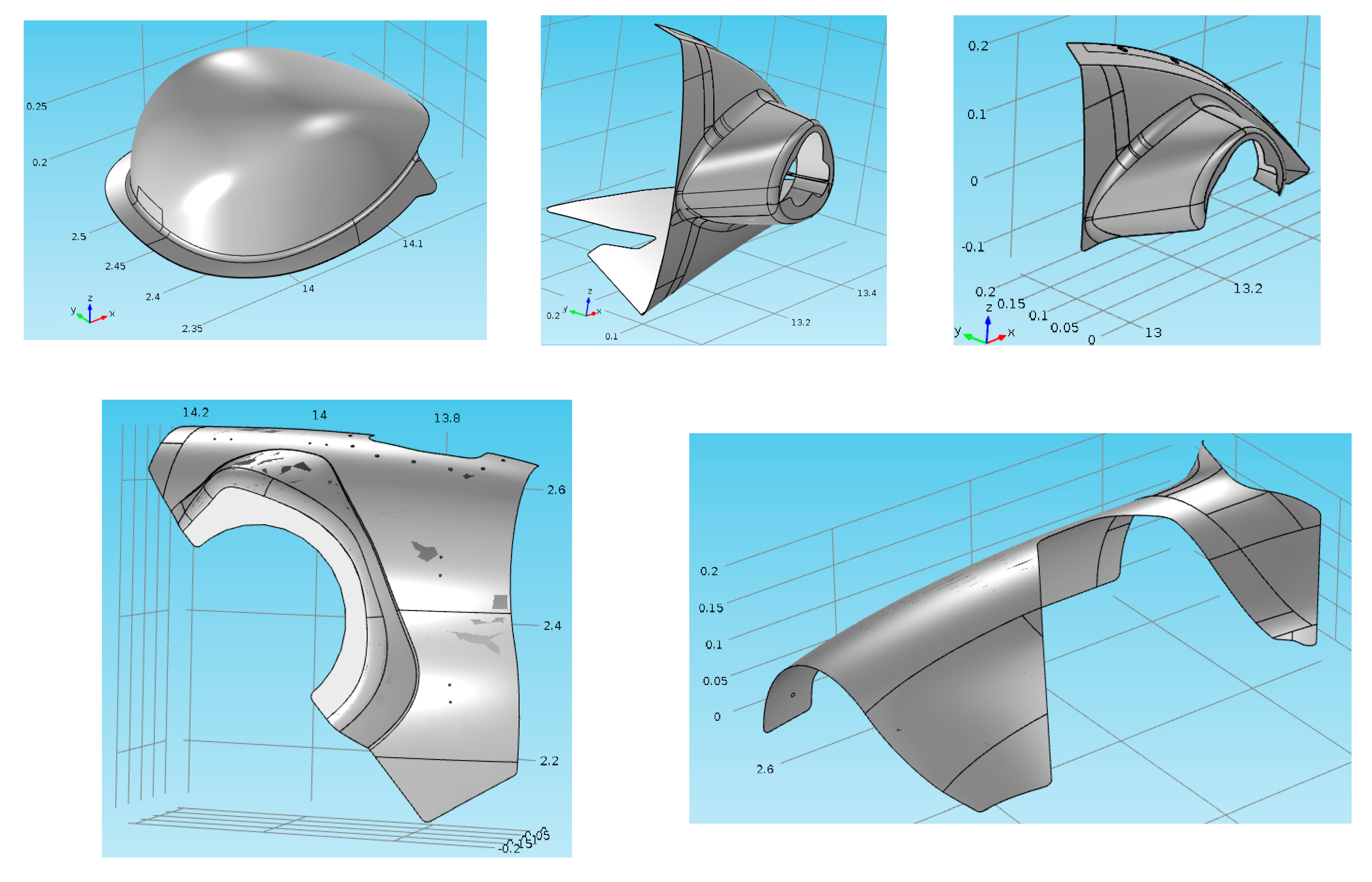
The study on the capabilities of the developed approach was carried out using CAD models of a group of rotorcraft composite structures with a geometry like thin-walled shells of complex shapes (see
Figure 12). The original CAD models were adjusted to correct topological errors (poor joining of the whole surface’s patches), which prevent high-quality finite element meshing, as well as some local simplifications to exclude mesh thickening in areas with increased curvature. This part of the work is very important because violation of C
0 or C
1 continuity of the surface and sharply changed FE meshing can cause front distortion and a change in the direction of its spreading.
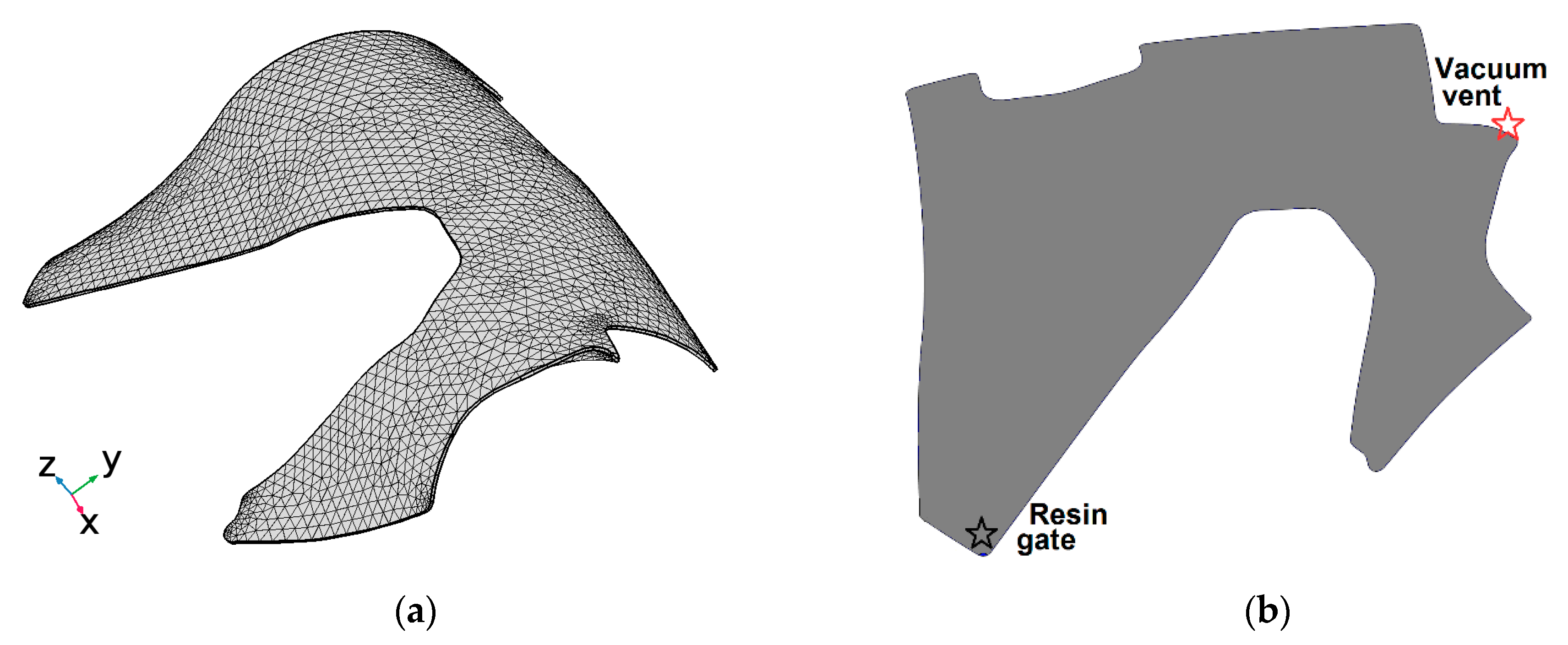
The remainder of this article presents and discusses the modeling of the infusion process in the last cowling shown in
Figure 13. The system modeling was implemented in Comsol Multiphysics environment, where the phase field in Equations (6) and (7), which are built-in simulation modes, were accepted as a ruling equation coupled with the modified Richards equation (Equation (14)), which was built in the coefficient form PDE mode. FE mesh and resin gate with vacuum vent locations are present in
Figure 13. All boundary conditions and the numerical value of the model parameters correspond to the above. The HPM tape 5 cm wide was laid around the part’s perimeter, which was taken into account at the HPM locations by increasing the preform permeability.
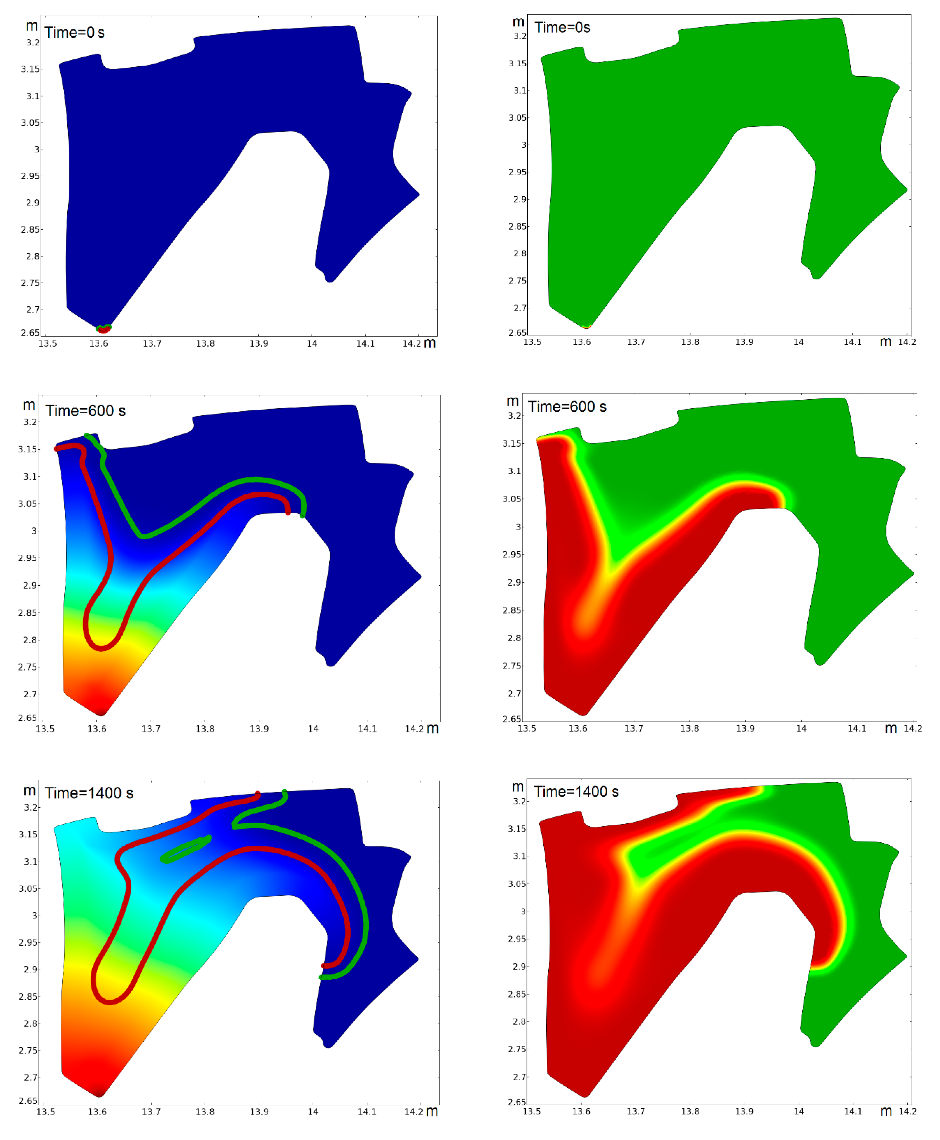
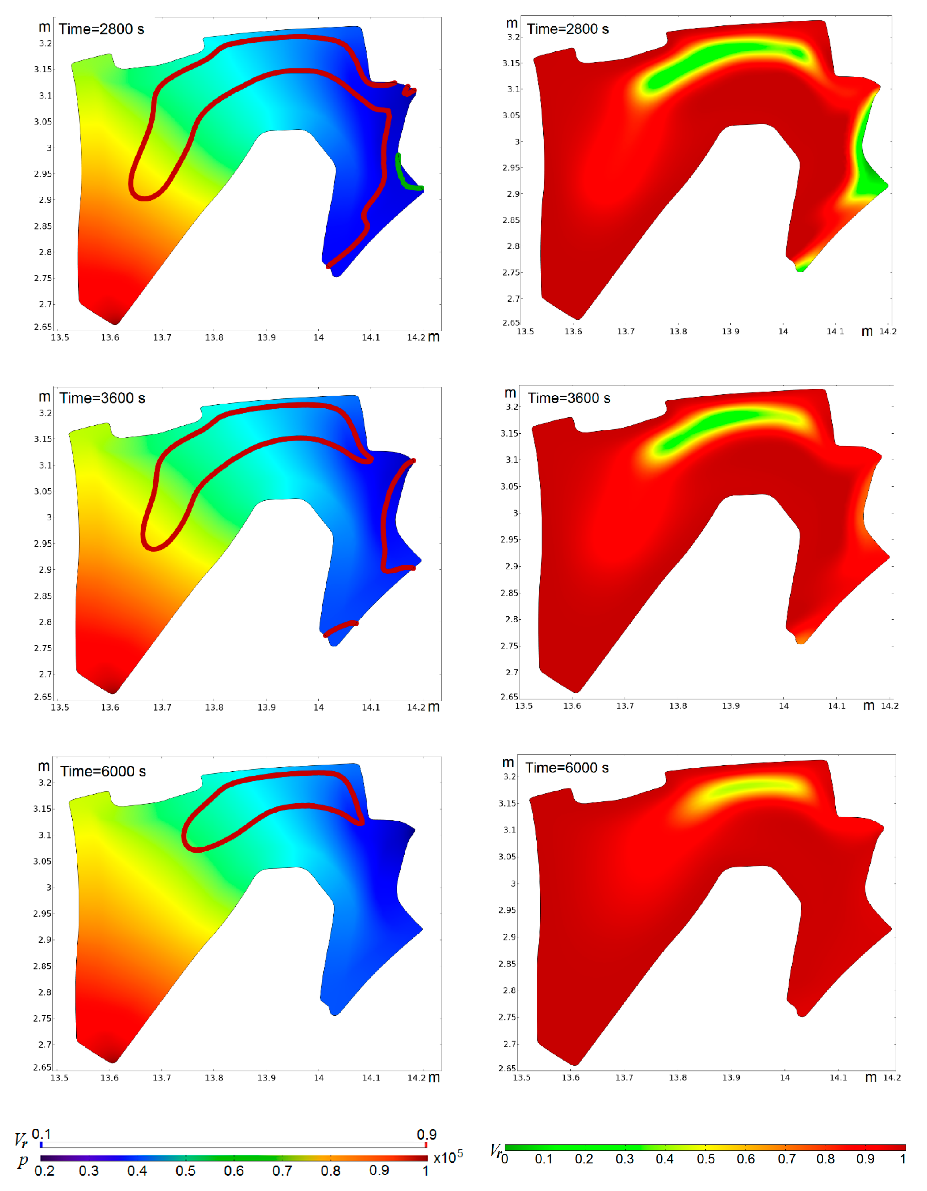
Some snapshots of the resin volume fraction and driving pressure distribution in the preform during model simulation are shown in
Figure 14. The left column of this Figure shows the plots of the resin pressure distribution in the preform combined with the lines of two
Vr levels: 0.1 and 0.9, whereas the right column contains the resin filling
Vr distribution plots at the different time instants. Several important features of the simulation can be identified when considering these images.
The use of HPM tapes located around the perimeter of the infusing preform can lead to a significant local expansion of the front of the resin (see time 600 s) and even to the formation of low pressure and saturation areas inside the resin flow front (see time 1400 s).
With the closure of some internal areas by an inner front, the filling of these areas with a resin gradually increases, although the nature of the pressure distribution inside such partially filled areas is not violated (see times 2800 s, 3600 s, 6000 s).
It can be explained by the real diffusion of the resin as well as by the mobility , which determines the time scale of diffusion in the Cahn–Hilliard equation (Equation (4)). Estimation of the actual magnitude of this mobility presents significant difficulties, but the occurrence of such closed contracting areas indicates the possibility of the formation of dry spots. A similar phenomenon is observed when the outer front approaches the protruding corners of the preform contour (see times 600 s and 2800 s). This slow mixing of two phases on the surface of their contact is inherent for all interacting systems. In real infusion processes, such mixing is constrained by an increase in air pressure inside the contracting empty area and a gradual increase in the viscosity of the resin over time under the influence of temperature due to polymerization. A detailed analysis, which is able to confirm or exclude the formation of an empty area in the real infusion process, can be performed using the algorithm processing the simulation results described below. Some justified guess-works can be made during simulation, which is very important when each simulation is controlled by an optimization algorithm that carries out the multiple calls of the forward problem with changed process conditions. Such guess-works should exclude from consideration potentially “dangerous” situations that contribute to the formation of dry spots.
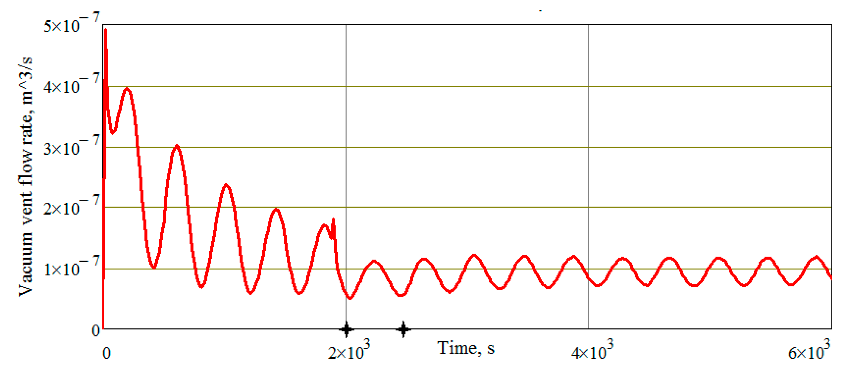
In order to detect the potentially forming the dry spots, two global variables have been calculated during simulation: the averaged pressure in partially filled areas of the preform Equation (19) and the flow rate through the vacuum vent’s boundary:
where
n is unit normal to the vent surface Σ.
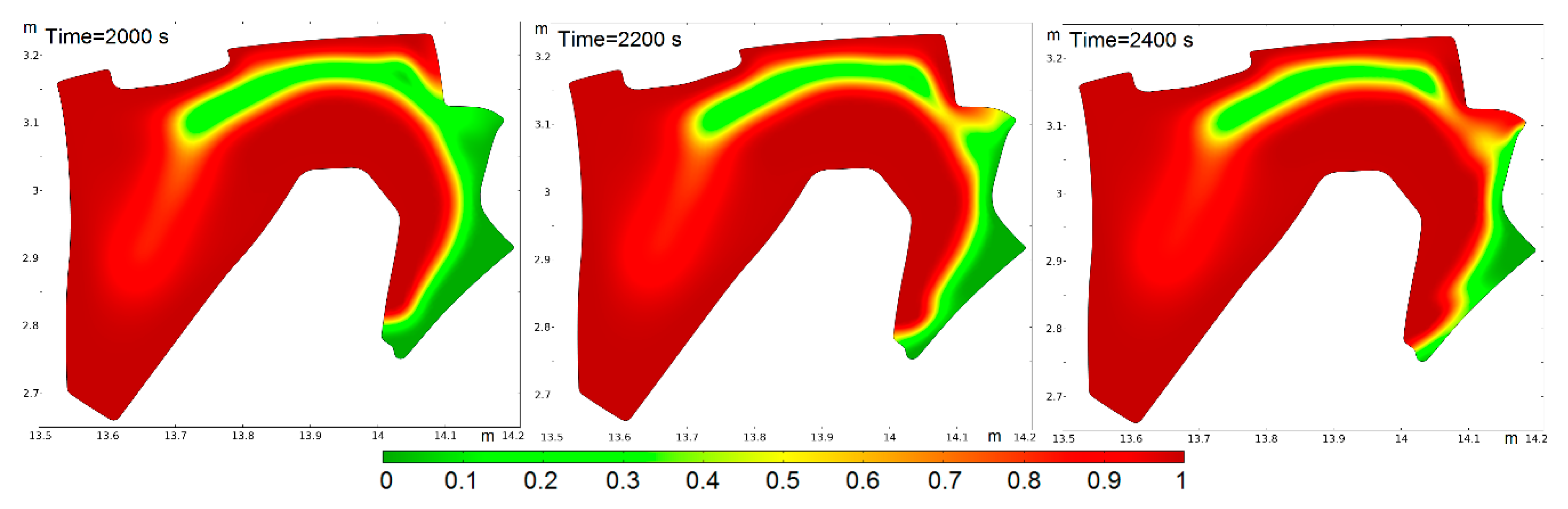
Figure 15,
Figure 16,
Figure 17 and
Figure 18 illustrate the changes in process infusion state at time interval 2000–2400 s. This time interval is noted by the cross markers on the time axis.
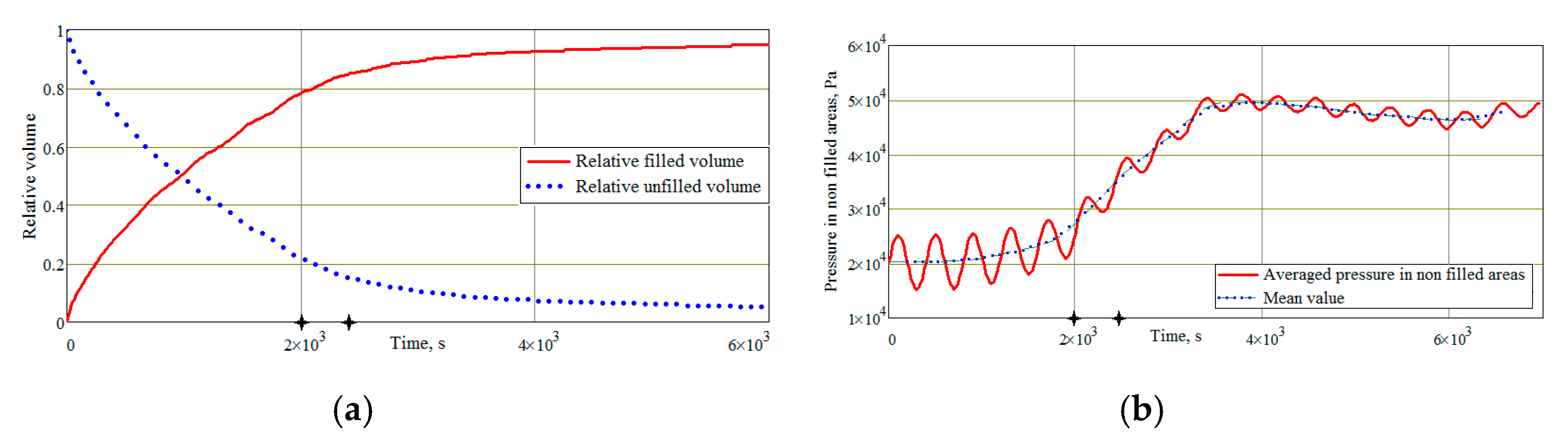
Figure 15 demonstrates a closing of the low resin filling region in the specified time interval. The state of the resin filling is illustrated in
Figure 16a, whereas the change of the averaged pressure in the partially filled regions surrounded by the resin volume fraction
Vr = 0.5 is present in
Figure 16b. One can see in
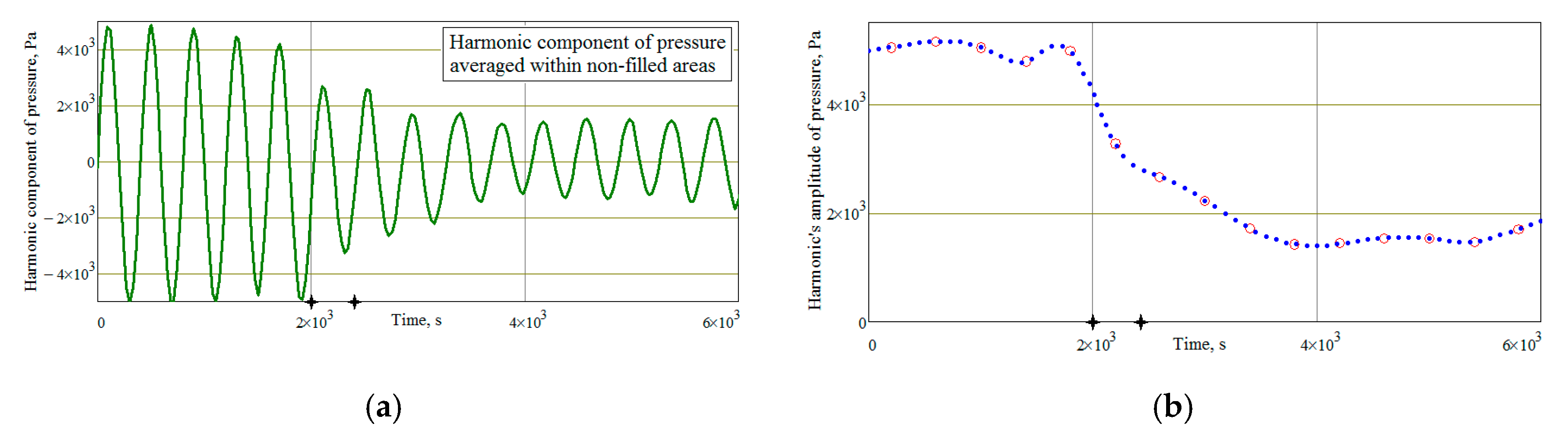
Figure 17 how the harmonic component’s amplitude of the pressure drops sharply during the separation of the closable region from the rest of the unfilled volume, in which the amplitude of the pressure oscillations is kept constant according to Equation (18). Such monitoring is performed during simulation, and it can signal the formation of potentially dangerous dry areas. Of course, the sensitivity of such a registration method depends on the magnitude of the closable volume: the larger this volume, the greater the change in the average amplitude of the pressure oscillations. Attention should also be paid to a sharp decrease in the vent’s air flow rate shown in
Figure 18, which can also serve as an additional source of information about the formation of a possible dry spot.
The considered results demonstrate that proposed computations can be used to exclude the suspicious modeling scenarios in which the formation of dry places is possible. However, a much more reliable conclusion about the process quality at its accepted conditions can be made using the algorithm processed the simulation results. The most important elements and results of this algorithm working in the MATLAB environment are described below.
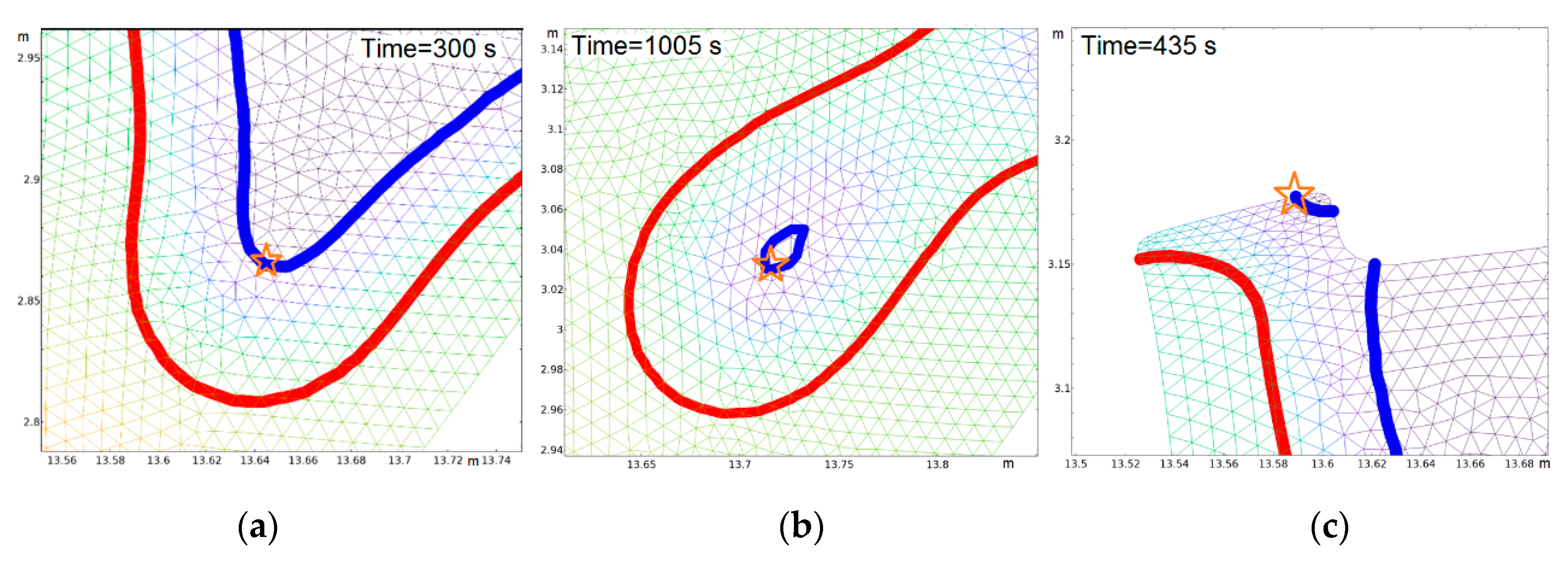
This algorithm includes the following sequential steps, which are illustrated for three different situations: (a) no dry spot formation, (b) dry spot is formed by the inner flow front and (c) dry spot is formed by the outer resin flow front (see
Figure 19).
After completing the FE solution, this algorithm imports the coordinates of all nodes together with the resin volume fraction and pressure in these nodes for all time steps during simulation. Next, the time instants
when the resin volume fraction first surpasses a value 0.1 are determined for all nodes of FE mesh (see
Figure 20a–c).
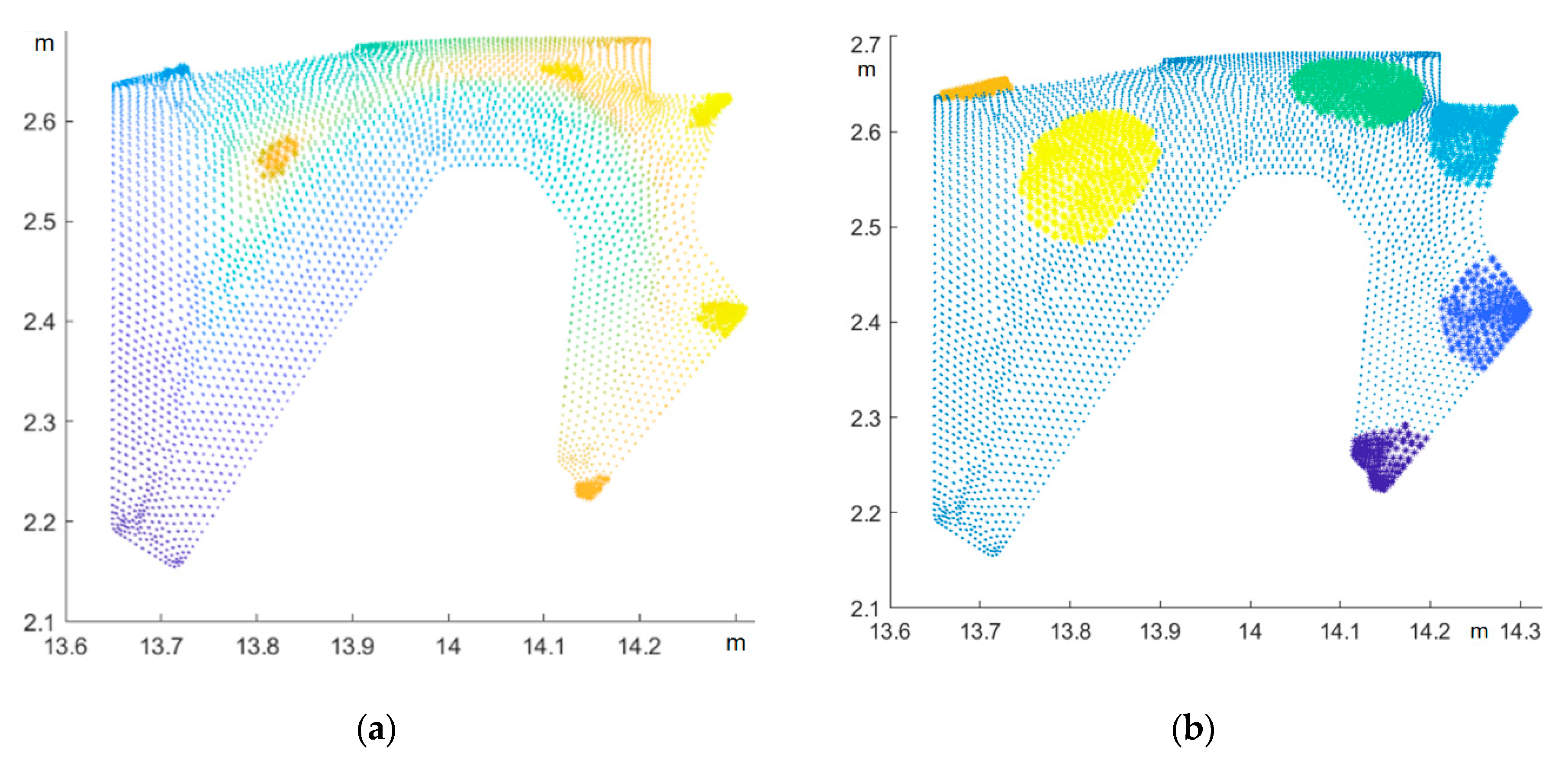
For these found nodes, their environment with filled nodes is determined and the identification of the arisen dry “traps” is made during the following steps (see
Figure 21). Then, a sorting all the trapped nodes and identifications of the dry spots separated from each other is performed.
Figure 22a demonstrates these separated spots, which are depicted by bold dots of various colors, and each dry spot is highlighted in its own color. Reconstruction of the closing resin front shapes (the original contour of the closing unfilled area) is performed by the analysis of
for all nodes belonging to the selected spots. These original contours of all closed spots are shown in
Figure 22b at the time instants of their closing.
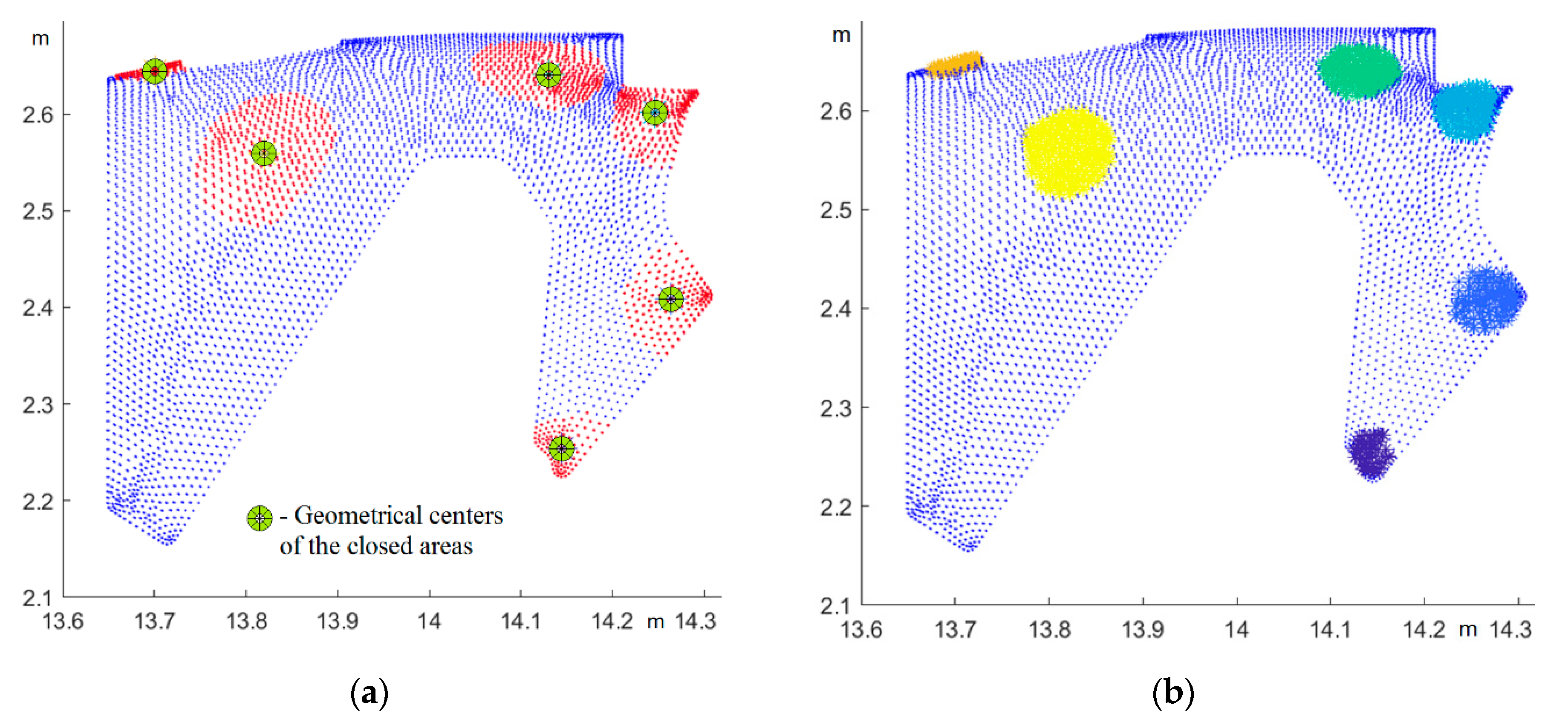
In order to estimate the changes for these closed unfilled areas and their volumes, two assumptions are accepted. The first is that the air in the closed areas obeys the gas law at the constant temperature
, and the second is that the contraction of such areas occurs around their geometric center. Therefore, the centers of the spots are determined, as highlighted in
Figure 23a, and then each area shrinks into a rounded shape so that the pressures inside and outside are equalized (see
Figure 23b). At these contraction deformations, a change of the nodes number inside the spot is calculated. The results of these two final steps of the algorithm are shown in
Figure 23.
Consequently, the considered MATLAB tool can be effectively used both for preliminary selection of the arrangement of resin gates and vacuum vents, their geometry and boundary conditions, and for a detailed analysis of the optimized technological solution that can be obtained using the above discussed FE-based tool for the vacuum infusion process simulation.

 ,
, 


