Article

Dynamic-DSO: Direct Sparse Odometry Using Objects Semantic Information for Dynamic Environments

1
School of Instrument Science and Engineering, Southeast University, Nanjing 210096, China
2
Key Laboratory of Micro-Inertial Instrument and Advanced Navigation Technology, Ministry of Education, Nanjing 210096, China
*
Author to whom correspondence should be addressed.
Appl. Sci. 2020, 10(4), 1467; https://doi.org/10.3390/app10041467
Submission received: 31 December 2019 / Revised: 14 February 2020 / Accepted: 18 February 2020 / Published: 21 February 2020
(This article belongs to the Special Issue Mobile Robots Navigation Ⅱ)

Abstract

:
Traditional Simultaneous Localization and Mapping (SLAM) (with loop closure detection), or Visual Odometry (VO) (without loop closure detection), are based on the static environment assumption. When working in dynamic environments, they perform poorly whether using direct methods or indirect methods (feature points methods). In this paper, Dynamic-DSO which is a semantic monocular direct visual odometry based on DSO (Direct Sparse Odometry) is proposed. The proposed system is completely implemented with the direct method, which is different from the most current dynamic systems combining the indirect method with deep learning. Firstly, convolutional neural networks (CNNs) are applied to the original RGB image to generate the pixel-wise semantic information of dynamic objects. Then, based on the semantic information of the dynamic objects, dynamic candidate points are filtered out in keyframes candidate points extraction; only static candidate points are reserved in the tracking and optimization module, to achieve accurate camera pose estimation in dynamic environments. The photometric error calculated by the projection points in dynamic region of subsequent frames are removed from the whole photometric error in pyramid motion tracking model. Finally, the sliding window optimization which neglects the photometric error calculated in the dynamic region of each keyframe is applied to obtain the precise camera pose. Experiments on the public TUM dynamic dataset and the modified Euroc dataset show that the positioning accuracy and robustness of the proposed Dynamic-DSO is significantly higher than the state-of-the-art direct method in dynamic environments, and the semi-dense cloud map constructed by Dynamic-DSO is clearer and more detailed.

Graphical Abstract

1. Introduction

SLAM (Simultaneous Localization and Mapping, with loop closure detection) and VO (Visual Odometry, without loop closure detection) are the key technologies of robot autonomous operation in unknown environments. In cases where prior information about the environment is unknown, SLAM and VO can establish an environment map when the robot is in motion and simultaneously provide the position of the robot in the map by using the camera mounted on the robot [1]. Due to the advantages of low hardware cost, not having to arrange the scene in advance, and making full use of the texture information of the environment [2,3], SLAM and VO have already become the focus of current research, and are widely used in unmanned driving, augmented reality, virtual reality and other fields [4,5]. According to the number and type of cameras, SLAM and VO can be divided into monocular, stereo and RGB-D configuration. As the monocular camera has the characteristics of simple structure and low hardware cost, the monocular SLAM or VO has captured significant attention from researchers.
According to different feature association methods, SLAM and VO can be divided into indirect methods (feature point methods) and direct methods. Indirect methods—represented by Mono-SLAM [6], PTAM [7] and ORB-SLAM2 [8], which rely on multi-view geometry—conduct feature point extraction and matching firstly, and then complete the state estimation by minimizing the reprojection error. These approaches achieve decent positioning accuracy and stability in rich-texture environments, and demonstrate a high robustness to light changes. However, the significant dependence on the number of feature points brings about low positioning accuracy and poor robustness in weak-texture environments. Feature extraction and matching are very time-consuming. Different from indirect methods that separate feature association and state estimation independently, direct methods represented by LSD-SLAM [9], SVO [10] and DSO [11] put them into a joint nonlinear optimization model. By constructing and minimizing the photometric error, feature association and state estimation are solved at the same time. Although indirect methods have been in the mainstream for a long time, the recent research progress in direct methods shows better accuracy and robustness, especially when there are not enough feature points due to the weak texture environment. The robustness in direct method comes from the joint estimation of system state and feature association as well as the ability to use non-corner pixels, corresponding to edges, or even smooth image regions (as long as there is sufficient image gradient).
However, most of the current SLAM or VO systems, whether direct methods or indirect methods have the assumption that the environment is static, meaning that the geometric distribution of objects in the scene should keep static when camera is in motion. Dynamic objects in the scene, such as pedestrians and driving cars, will destroy the feature association and state estimation, reduce the positioning accuracy and system robustness or even cause system failure. Since, in most fields—such as automatic driving and intelligent robots—where SLAM system works in reality, dynamic objects are ubiquitous. How to improve the positioning accuracy and robustness of SLAM or VO systems in dynamic environments has become a hot issue in recent years.
Several scholars combine the traditional indirect method with deep learning [3,12,13,14,15,16], which significantly improves the positioning accuracy and robustness of the indirect visual SLAM or VO system in the dynamic environments. However, the direct method, which is another branch of SLAM or VO in parallel with the indirect method and shows better accuracy and robustness in the weak texture environment, is also interfered by dynamic objects. In direct methods, feature association and state estimation are jointly solved, which is entirely different from the independent solution strategy in indirect methods.
In this paper, Dynamic-DSO is proposed. We focus on reducing the impact of dynamic objects in direct visual odometry by combining semantic segmentation networks with DSO [11], which are the state of the art of current direct methods. We applied convolutional neural networks to the input image to generate the pixel-wise semantic information of dynamic objects. Then, we filtered out the dynamic candidate points in the process of keyframes candidate points extraction based on semantic information of dynamic objects. In pyramid motion tracking model, the photometric error calculated by the projection points in dynamic region of subsequent frames are removed from the whole photometric error. In order to obtain the precise camera pose, the sliding window optimization which neglects the photometric error calculated in dynamic region of each keyframe is applied. The proposed Dynamic-DSO exploits the semantic information in the image, significantly improves the positioning accuracy and robustness of direct method in dynamic environments. The contributions of this work are as follows:
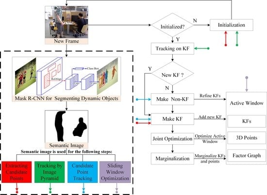
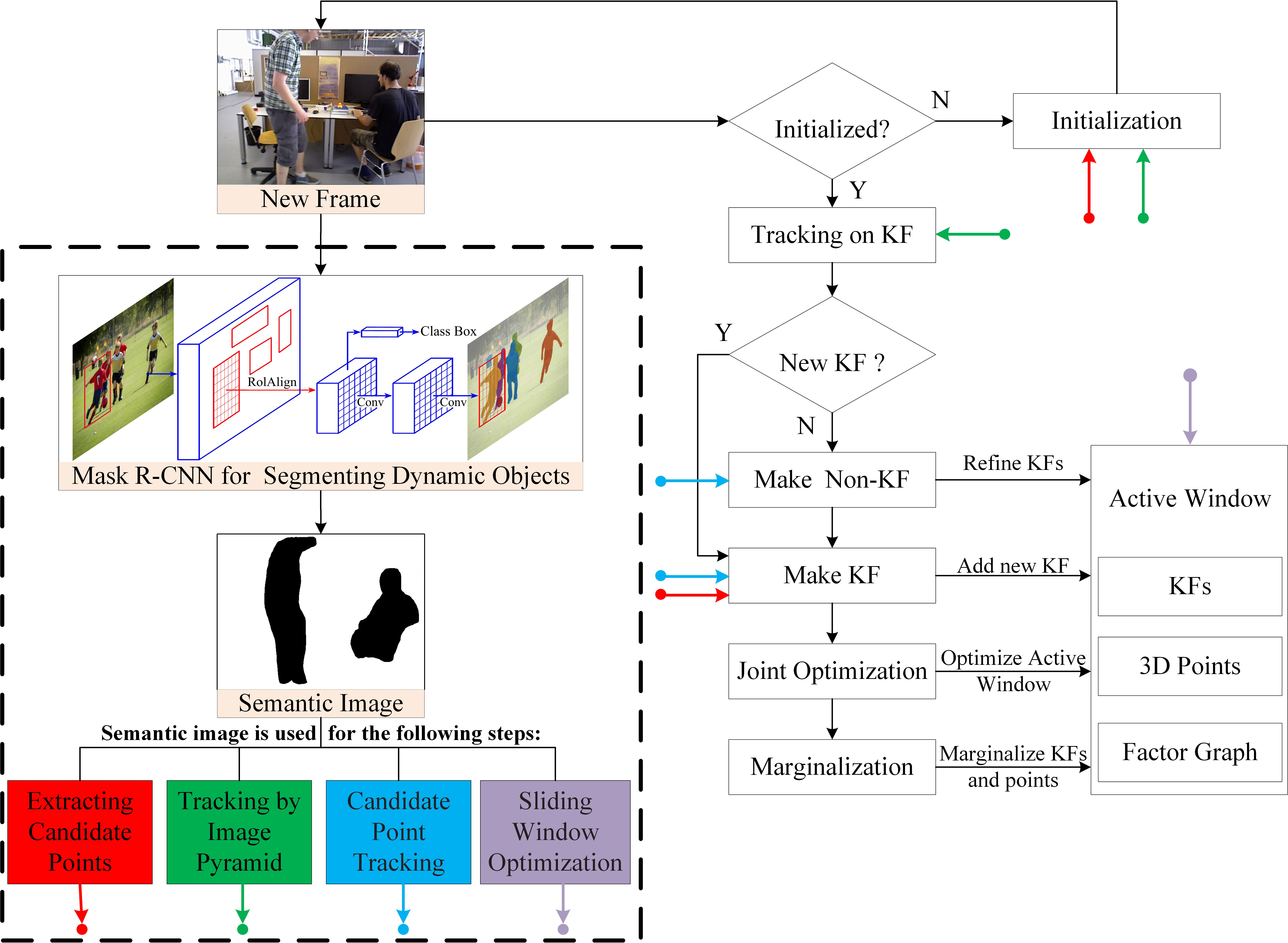
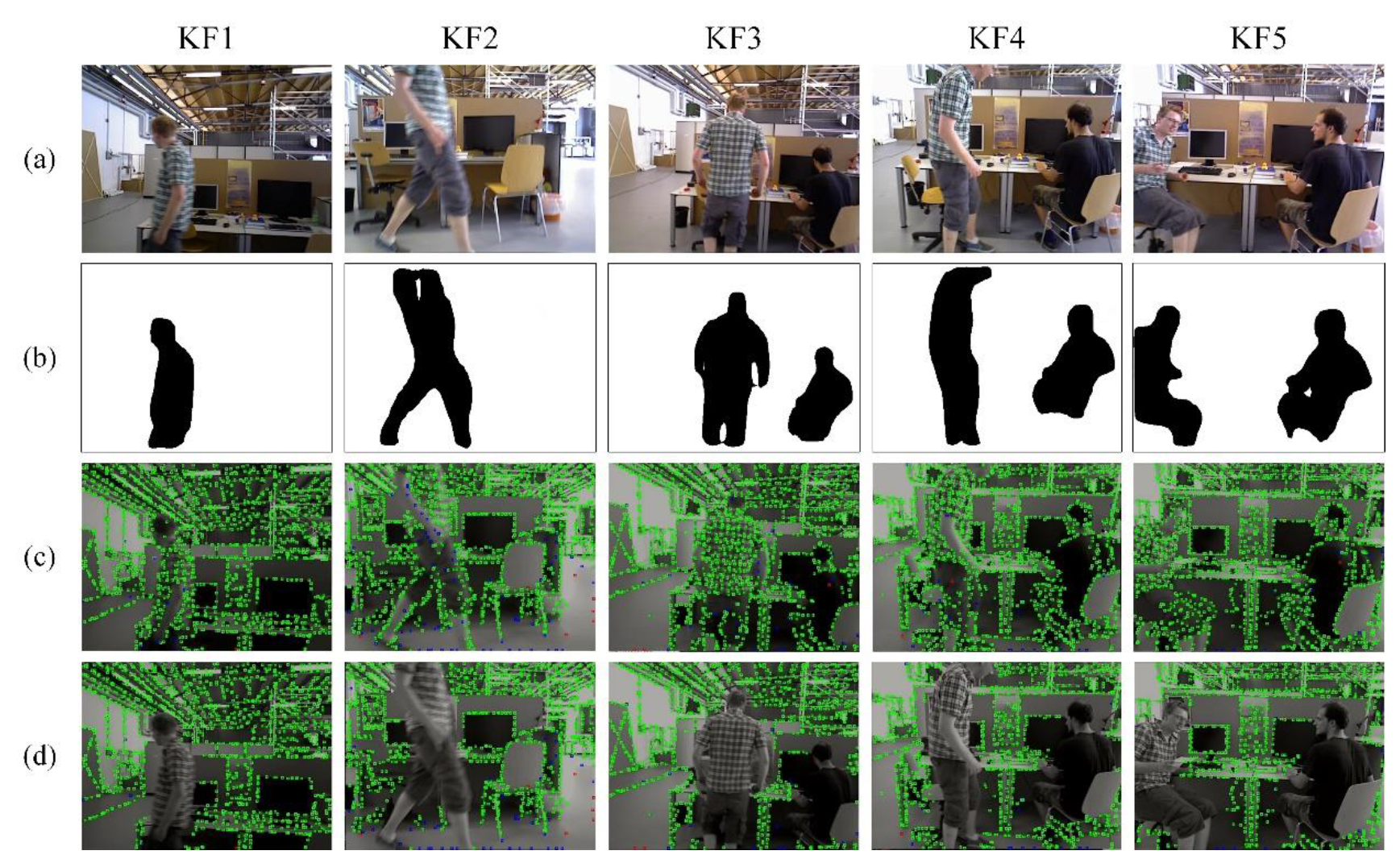
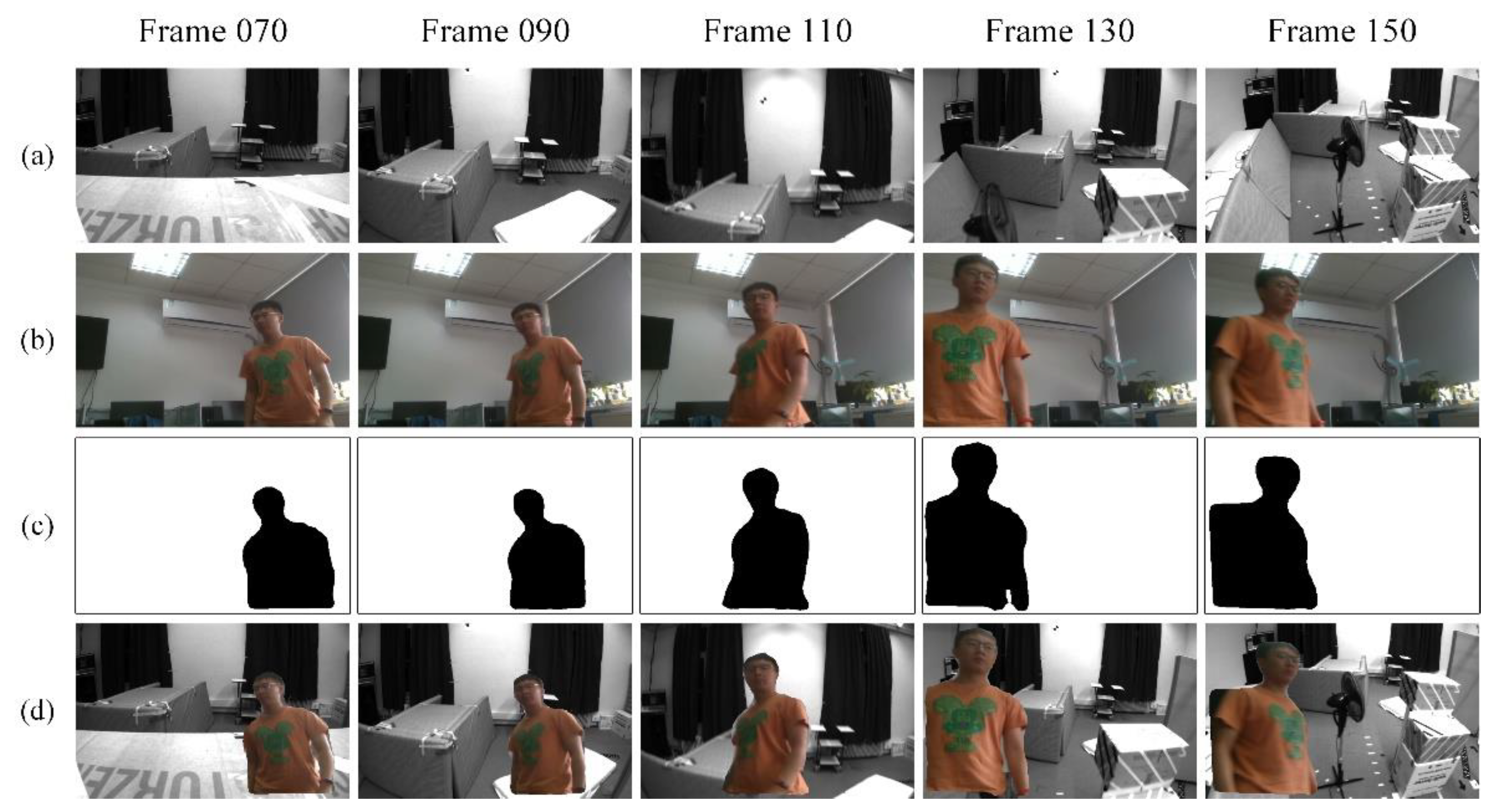
  • The proposed system is entirely based on the direct method. We exploited the semantic information of dynamic objects and eliminated the dynamic candidate points from keyframes, which ensured that only static candidate points were reserved in the tracking and optimization process.
  • In the pyramid motion tracking model and sliding window optimization, the photometric error calculated by the projection points in the image dynamic region are removed from the overall residuals, resulting in more accurate pose estimation and optimization.
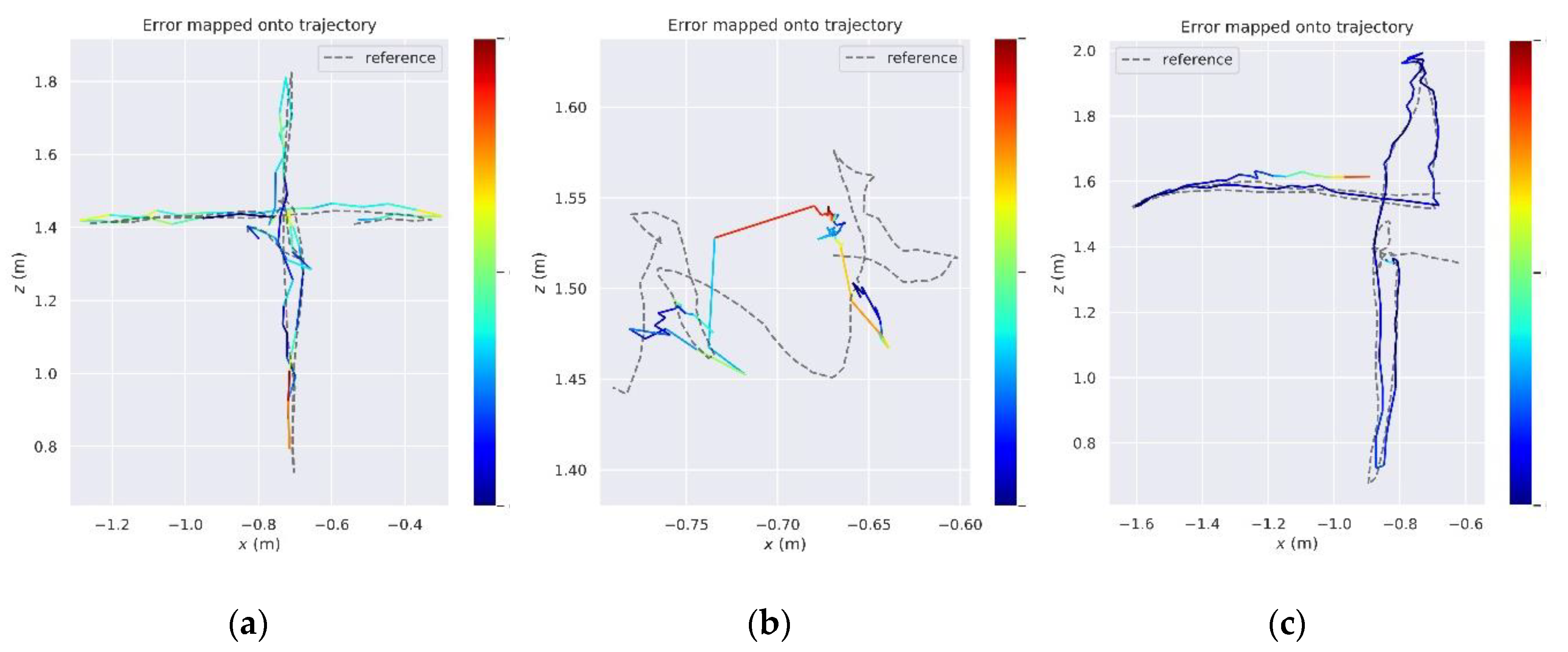
  • We evaluated the proposed system on the public TUM dynamic dataset and the modified Euroc dataset, and achieved robust and accurate results.
The rest of this paper is organized as follows. Section 2 introduces the related work. Section 3 introduces the framework of Dynamic-DSO. In Section 4, the main work is described and demonstrated in detail. In Section 5, a series of comparative experiments are reported to analyze the performance of the proposed method in dynamic environments. Finally, conclusions and future work are discussed in Section 6.

2. Related Work

Before deep learning was widely used in SLAM and VO, several researchers applied geometric constraints or statistic methods to deal with the problem of SLAM or VO systems working in dynamic environments. In 2007, Charles et al. [17] proposed a method that integrating the least-squares formulation and sliding window optimization with generalized expectation maximization. Both dynamic and static objects are directly incorporated into the estimation to maintain a consistent estimate. In 2012, Walcott-Bryant et al. [18] presented Dynamic Pose Graph SLAM (DPG-SLAM), which uses incremental smoothing and mapping (iSAM) as the underlying SLAM state estimation engine to maintain an up-to-date map even though the environment is changing. In the same year, Zou et al. [19] proposed a novel CoSLAM. By equipping multiple cameras on different platforms which move independently but work together, the system completes the intercamera pose estimation and intercamera mapping in dynamic scenes. It works robustly, but the video data must be processed offline. Kerl et al. [20] presented a probabilistic formulation in 2013, which employs sensors and motion models with custom probability distributions to complete the camera motion estimation from RGB-D images robustly and directly. In 2015, a dense 3D SLAM using Kinect in dynamic scene was presented by Bakkay et al. [21]. Based on a constant motion model, pixels whose absolute velocity exceeds the threshold probably belong to moving objects and are taken as seed segmentation. Then a region growing procedure is performed to identify dynamic regions by adapting these seeds. Li et al. [22] proposed a RGB-D SLAM method based on depth edge for dynamic environments in 2017. Only depth edge points are used to estimate the camera motion. The static weight, which represents the possibility of a point belonging to the static region, is combined with the intensity assisted iterative closest point (IAICP) algorithm to handle highly dynamic environment. In 2018, Bahraini et al. [23] presented a novel method to segment and track dynamic objects in dynamic environments. By using ML-RACSAC, the states which include velocity and the position of multiple moving objects can be robustly estimated in an unknown environment.
With the rapid development of deep learning technology in various fields, especially in the field of computer vision such as object detection and semantic segmentation, quite a few researchers have tried to make use of the image semantic information extracted by deep learning technology to improve the performance of SLAM or VO in dynamic environments in recent years, especially in the past two years. In 2017, Chen el al. [12] combined CNN objection detection with feature-based monocular SLAM. The system adopts YOLOv2 [24] to detect the dynamic objects in the scene. Then the feature points belonging to dynamic objects are eliminated and static features are remained for further data association and graph optimization. In 2018, Bescos et al. [13] proposed a front end to segment dynamic content by using multi-view geometry and Mask R-CNN [25]. They combined this front end with ORB-SLAM2 [8] to improve the robustness of SLAM in monocular, stereo and RGB-D configurations. In the same year, DS-SLAM was presented by Yu et al. [14]. The system integrates SegNet [26] and moving consistency check to detect dynamic objects and build a dense semantic 3D octo-tree map. Zhang et al. [15] also proposed a semantic SLAM for dynamic environments based on object detection and an improved octo-tree map in 2018. In 2019, there are also some researchers carrying out some superior work. Cui et al. [3] proposed Semantic Optical Flow SLAM (SOF-SLAM), which is built on RGB-D mode of ORB-SLAM2 [8]. The pixel-wise semantic segmentation obtained from SegNet [26] is used as a mask in the semantic optical flow to calculate a credible fundamental matrix, then the dynamic features are removed on the basis of the matrix. Xiao et al. [16] presented a semantic monocular method combining the object detection. SSD object detector [27] is constructed to detect dynamic objects in detection thread at semantic level.
All of the above proposed methods based on deep learning are aimed at indirect method (feature points method), which achieve accurate camera pose estimation and high robustness of the indirect visual SLAM or VO system in the dynamic environments. As far as the current research progress is concerned, research into problems about direct methods in dynamic environments is still rare.

3. Framework of Dynamic-DSO

The framework of Dynamic-DSO is composed of an image preprocessing model and a direct VO. In the image preprocessing stage, we use the semantic segmentation technology in deep learning to segment the dynamic objects, and obtain the prior information of the dynamic objects in the input image. The prior information of the dynamic objects is then used to enhance the candidate point extraction, frame tracking, and back-end optimization in VO. VO is responsible for tracking the camera motion and constructing a semi-dense map of the environment. Details of VO are provided in Section 3.1. Figure 1 shows the overall framework of the proposed Dynamic-DSO.

3.1. Direct Visual Odometry

Dynamic-DSO is based on DSO [11], which is the state of the art in direct visual odometry. DSO adopts the direct sparse model to jointly optimize the camera pose, camera internal parameters, inverse depth of points by a sliding window. It includes a front-end and a back-end. The front-end is responsible for initialization, camera pose tracking, and the back-end is used for sliding window optimization. The details of the front-end and back-end are described as follow.

3.1.1. Front-End

The front-end part handles the following:
Candidate point extraction: DSO extracts candidate points from the first frame in initialization process and the keyframes selected in frame tracking process. These candidate points will be continuously tracked during the movement of the camera and participate in the pose solving process.
In dynamic environments, if points in the dynamic area and in the static region participate in the calculation and optimization of photometric error together, it will break the optimization direction, resulting in the decline of pose estimation and mapping accuracy. Dynamic-DSO uses the method described in Section 4.1 to extract candidate points in dynamic environments.
Frame tracking: The current frame adapts the nearest reference keyframe for motion tracking. The constant velocity model and the traditional two frame image alignment method are used to achieve the course-to-fine tracking on the multi-scale pyramid model, and the pose of current frame is obtained by minimizing the photometric error between current frame and reference keyframe.
In Section 4.2, we apply image semantic information to the traditional pyramid motion tracking model to reduce the impact of dynamic objects on tracking accuracy.
Candidate point tracking: The process exists in both keyframes and non-keyframes. For an immature point obtained from the keyframe, DSO projects it to the current frame according to the relative pose and the initial inverse depth, and calculates the direction of epipolar line. The position of the projection point with the smallest photometric error in the current frame is obtained by epipolar search, then the best matching is obtained by minimizing the photometric error with the Gauss–Newton method. After obtaining the best match, the inverse depth and co-variance of the immature point are calculated to constrain the search interval of subsequent frames, as described in [11].
For dynamic environments, since the prior information of dynamic objects has been obtained in Dynamic-DSO, if the best match position of the immature point is in the dynamic area of current frame, the inverse depth of this point will not be recovered. Then the point will be set as the outer point, as described in Section 4.3.
Keyframe Creation: Similar to ORB-SLAM2, we take many keyframes (around 5-10 keyframes per second), then sparsify them afterwards through the early marginalization of the redundant keyframes. Three terms are calculated to determine if a new keyframe is required: mean square optical flow ( f : = ( 1 n i = 1 n p p 2 ) 1 2 ), mean flow without rotation ( f t : = ( 1 n i = 1 n p p t 2 ) 1 2 ) and relative brightness factor between two frames ( a : = | log ( e a j a i t j t i 1 ) | ). When f , f t and a satisfies the following relationship, the current frame is selected as a new keyframe:
w f f + w f t f t + w a a > T k f
where w f , w f t and w a are the weighting terms.
Marginalization: The step decides which frames and points should be marginalized. A keyframe will be marginalized if the number of points which are visible in the latest frame is less than 5%. If the number of keyframes exceeds N f (always fixed at 7), then the keyframe, which is far from current frame and close to any other keyframes should be marginalized.

3.1.2. Back-End

The back-end performs a continuous sliding window optimization which usually contains 5–7 keyframes. The full photometric error Ephoto is optimized using the Gauss–Newton method. The calculation of E p h o t o is described as follows:
For a single point p in the reference frame I i , the photometric error when it is projected onto the target frame I j is:
E p j = p N p w p ( I j [ p ] b j ) t j e a j t i e a i ( I i [ p ] b i ) γ
where p is the projection of point p on frame I j , t i and t j are the exposure time for I i and I j , . γ represents the Huber norm, a i , a j , b i , b j are brightness transfer function parameters, N p is the residual pattern with eight surrounding neighbors described in [11], w p is the weighting factor given by following:
w p = c c 2 + I i ( p ) 2 2
where c is the camera intrinsics.
The projection process can be described as:
p = c ( R c 1 ( p , d p ) + t ) [ R t 0 1 ] : = T j T i 1 ,
where d p is the point’s inverse depth of point p , T i and T j are the poses of the involved frames I i and I j .
The full photometric error E p h o t o over all keyframes and points can be given by:
E p h o t o = i F p P i j o b s ( p ) E p j
where F is the set of all keyframes in the sliding window, P i is the set of all the points in keyframe I i , o b s ( p ) is the set of the keyframes in which the point p is visible.
In order to reduce the impact of dynamic scenes, Dynamic-DSO modifies the photometric error model by using the prior information of dynamic objects obtained from the sematic images of all keyframes. It is described in Section 4.4 in detail.

4. Methodology

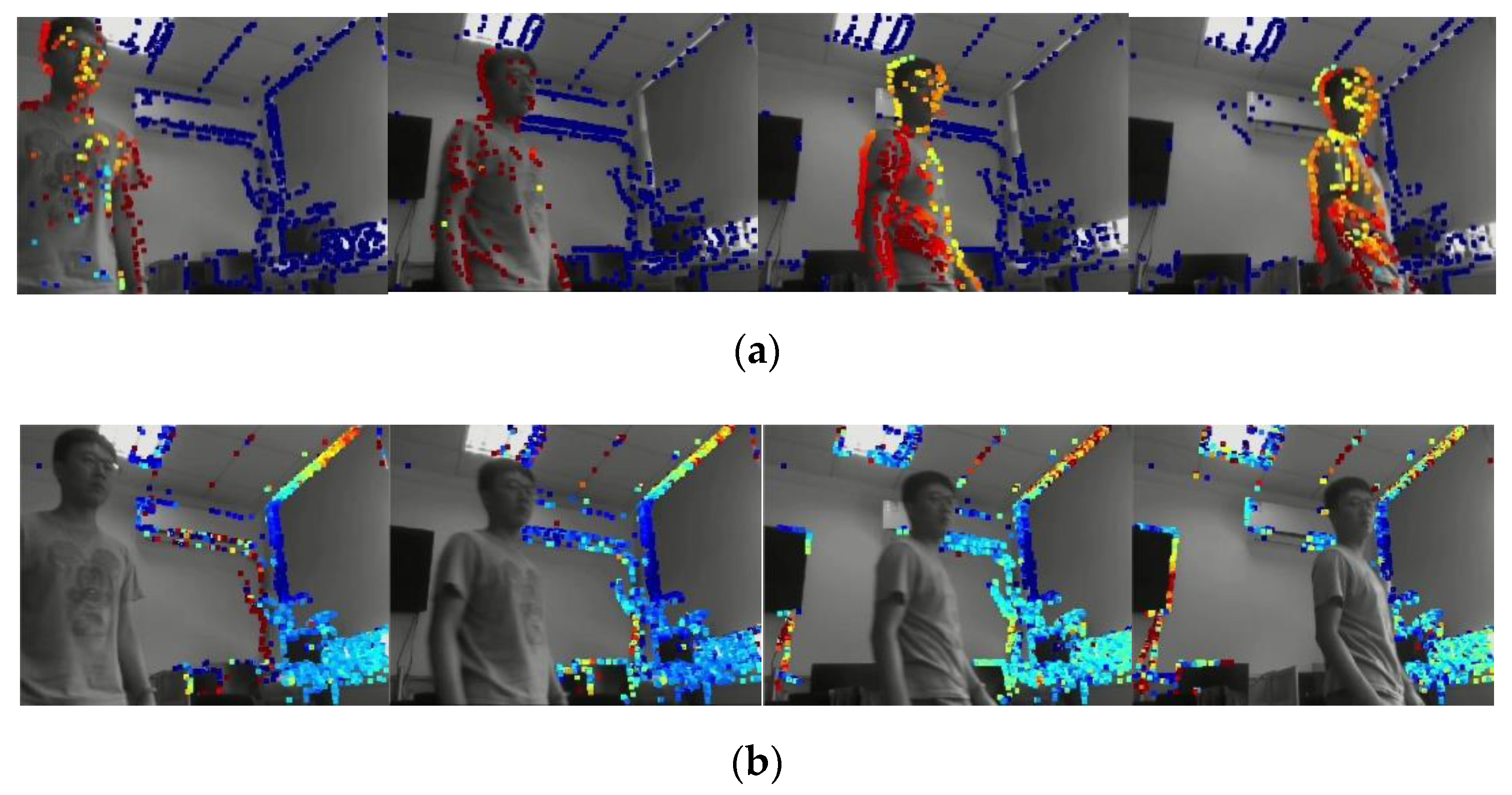
4.1. Candidate Points Extraction Based on Image Semantic Information

Different from DSO uniformly extracting candidate points from the image, we extract candidate points—taking into account the prior information of the dynamic objects in the image. Based on the candidate points extraction result of DSO, we first use CNNs to complete the semantic segmentation of the input image. Then the dynamic region of the image is determined by the semantic information of each segmented region, meaning that the prior information of the dynamic objects is obtained. Finally, the candidate points in dynamic regions are filtered out, and only the candidate points in static regions are preserved.

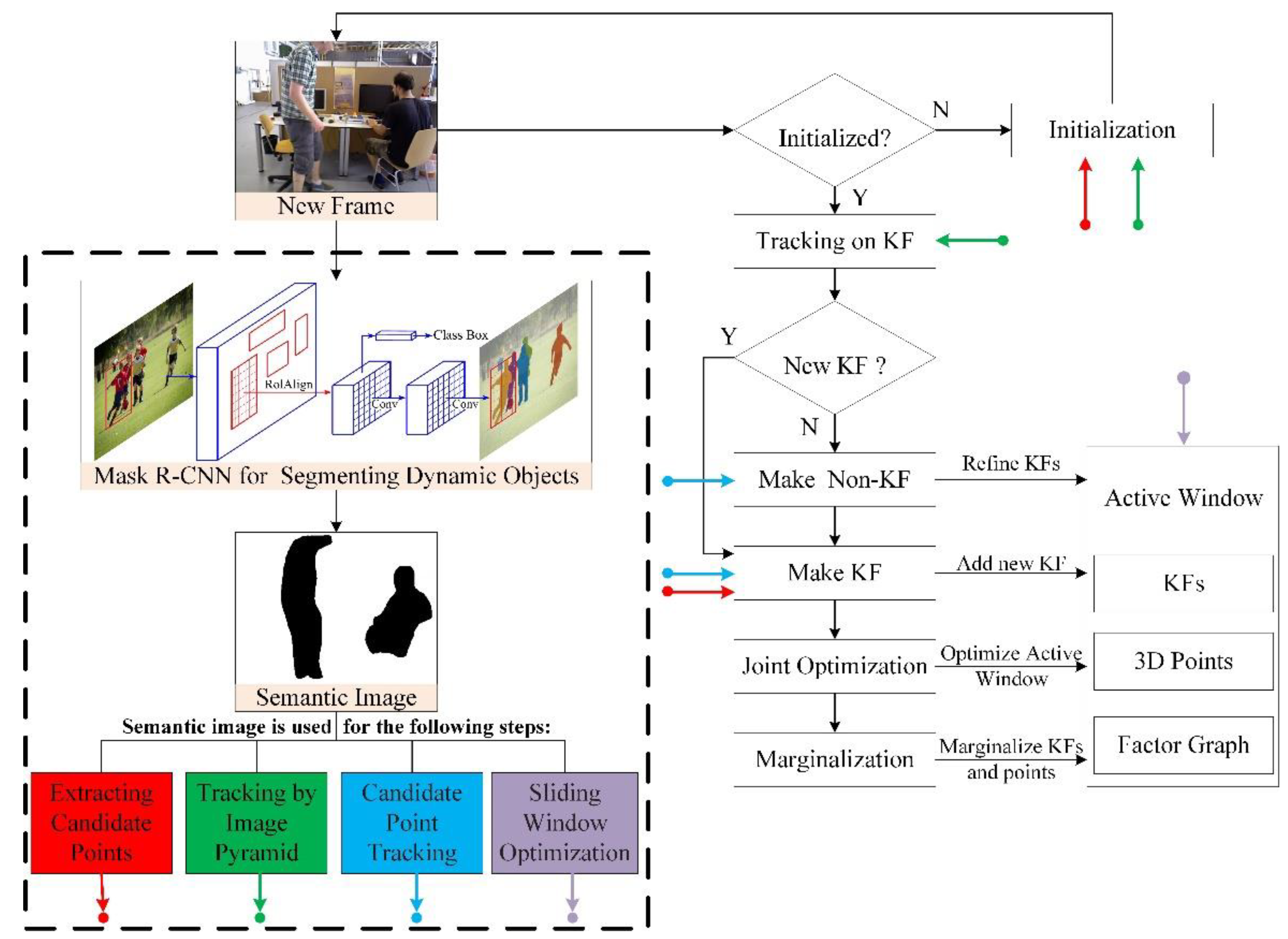
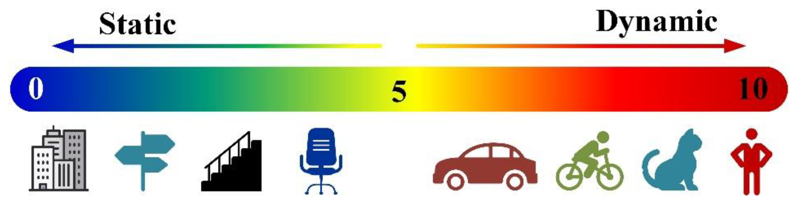
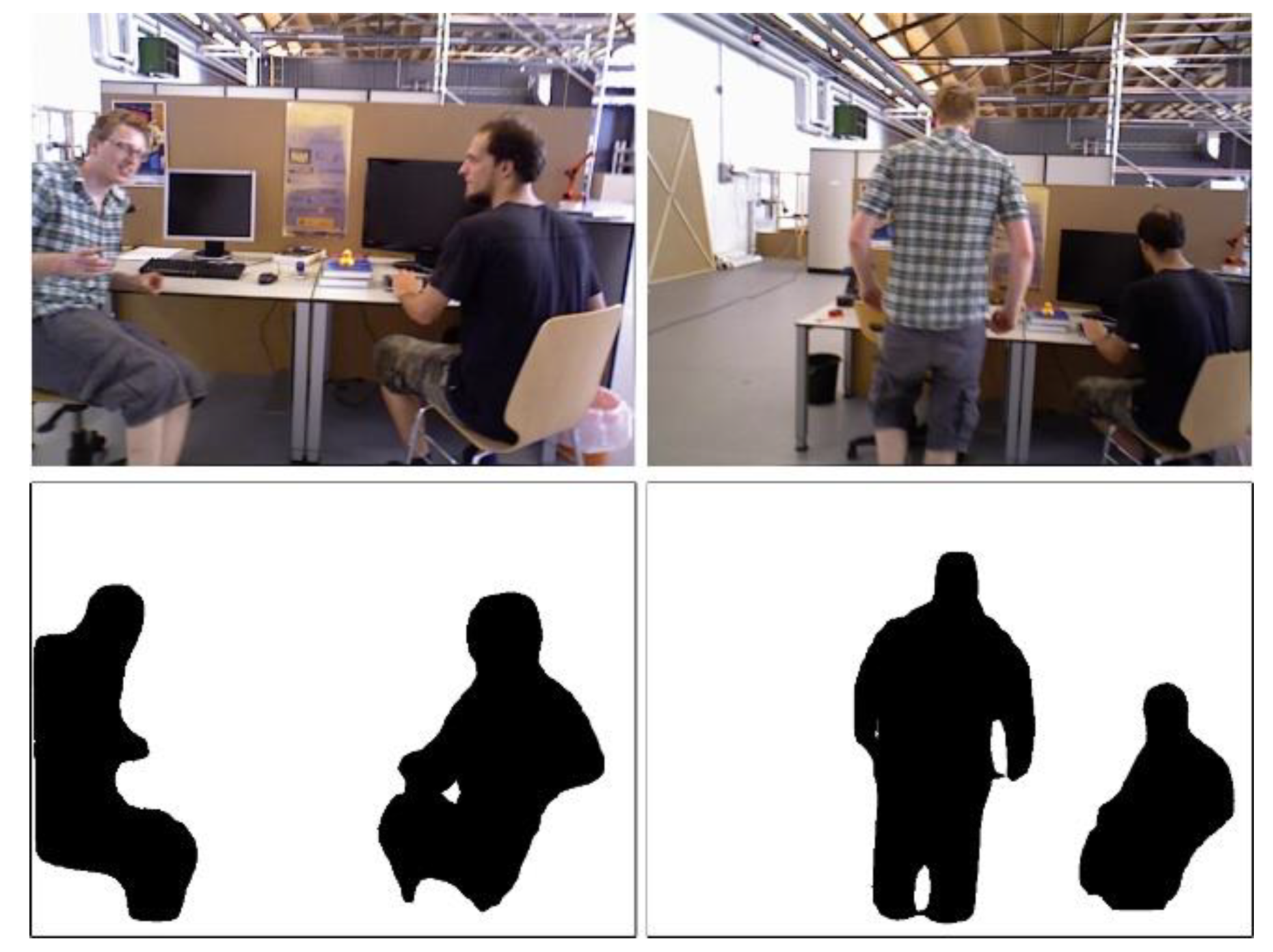
4.1.1. Dynamic Objects Segmentation Based on CNNs

We use CNNs to segment the input image and obtain the pixel-wise semantic information. In this paper, we choose Mask R-CNN [25], which is the state of the art in the field of image instance segmentation. It can obtain high quality pixel-wise semantic information and the instance label of each segmentation region. In the process of candidate points extraction, we only use the pixel-wise semantic information. In future work, the instance labels may be used for tracking different dynamic objects in the image. We adapt the TensorFlow version implemented by Matterport [28].
According to the prior experience of human life, we score the possible dynamic degree of an object in the real scene from 0 point (static) to 10 point (dynamic), and set a threshold artificially. When the score exceeds the threshold, meaning that it is a dynamic object, otherwise we consider it as a static object. The idea is to segment objects that may be dynamic or movable (e.g., people, bicycles, cars, motorcycles, airplanes, buses, trains, trucks, boats, birds, cats, dogs, horses, sheep, cattle). We consider that for most scenes, dynamic objects that may appear are included in the above list. Figure 2 shows the approximate score of common objects.
The input of Mask R-CNN is an RGB image with m × n × 3 dimension, and the output of the network is a matrix with m × n × l dimension, where l represents the number of objects to be detected in the image. For each output channel, we will get a binary mask. By synthesizing the output of all channels into one, the pixel-wise semantic results containing all the dynamic objects in the input image are obtained. Figure 3 shows the segmentation results for indoor pedestrians.

4.1.2. Candidate Points Extraction

For each input image I , the corresponding semantic image I s e m containing dynamic objects information can be get according to Section 4.1.1. For candidate points extraction from keyframes, the image is split into d × d blocks firstly. Then, we calculate a region adaptive threshold for each block, and select the points with the largest gradient and exceeding the gradient threshold as the candidate points. In order to obtain information from weak intensity changes, such as smooth changes in lighting on white walls, some points with smaller gradients from areas without high gradient points are selected. We follow the approach as DSO [11] described and select pixels with a lower gradient threshold and an increased d .
For the candidate point p extracted from image I , we map it to the semantic image I s e m . If the mapping position is in the dynamic region, then the point p will be discarded, otherwise we reserve it. Since the edge of image segmentation results maybe not very accurate, we not only consider the position of point p , but also judge the four adjacent points of p . Only when these five points are not in the dynamic region, p is reserved as a candidate point. A summary of the whole extraction method is given in Algorithm 1.
Algorithm 1: Candidate points extraction based on image semantic information
Input: The original image I, the semantic image Isem, the number of points required: N;
Output: The set S of candidate points, the number of selected points Nsel;
  Initialize: S = { } , Nsel = 0, k = 1;
  while Nsel < N do
   for k <= 4 do
    Split image I into kd × kd blocks;
    for each block do
     Select a point p with the highest gradient which surpass the gradient threshold;
     if no selected point in this block then
      Select a point p with the highest gradient which surpass the lower gradient threshold;
     end if
     if Isem [p] != 0 then
      Find the points p1, p2, p3, p4, where they are distributed above, below, left and right at p with the pixel interval D;
      if (Isem [p1] != 0 && Isem [p2] != 0 && Isem [p3] != 0 && Isem [p4] != 0 ) then
       Append point p to set S;
      end if
     end if
    end for
    k = 2 × k;
   end for
   Nsel = Nsel + the number of selected points;
  end while

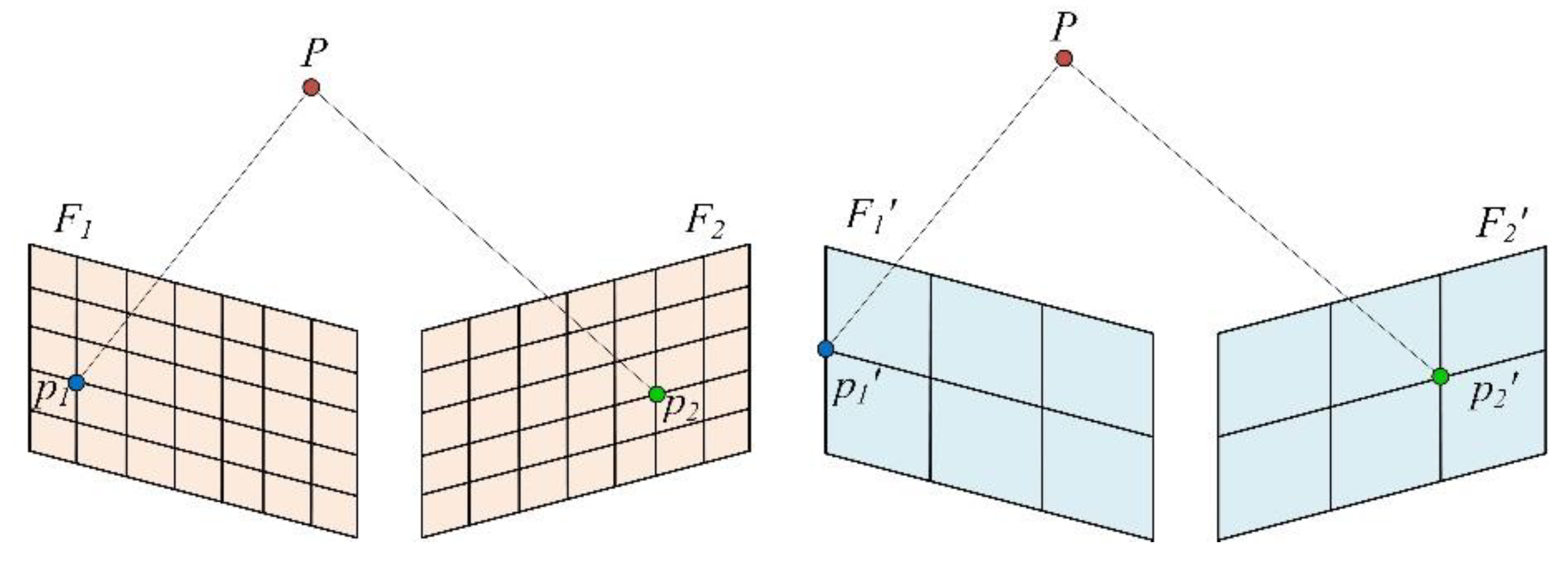
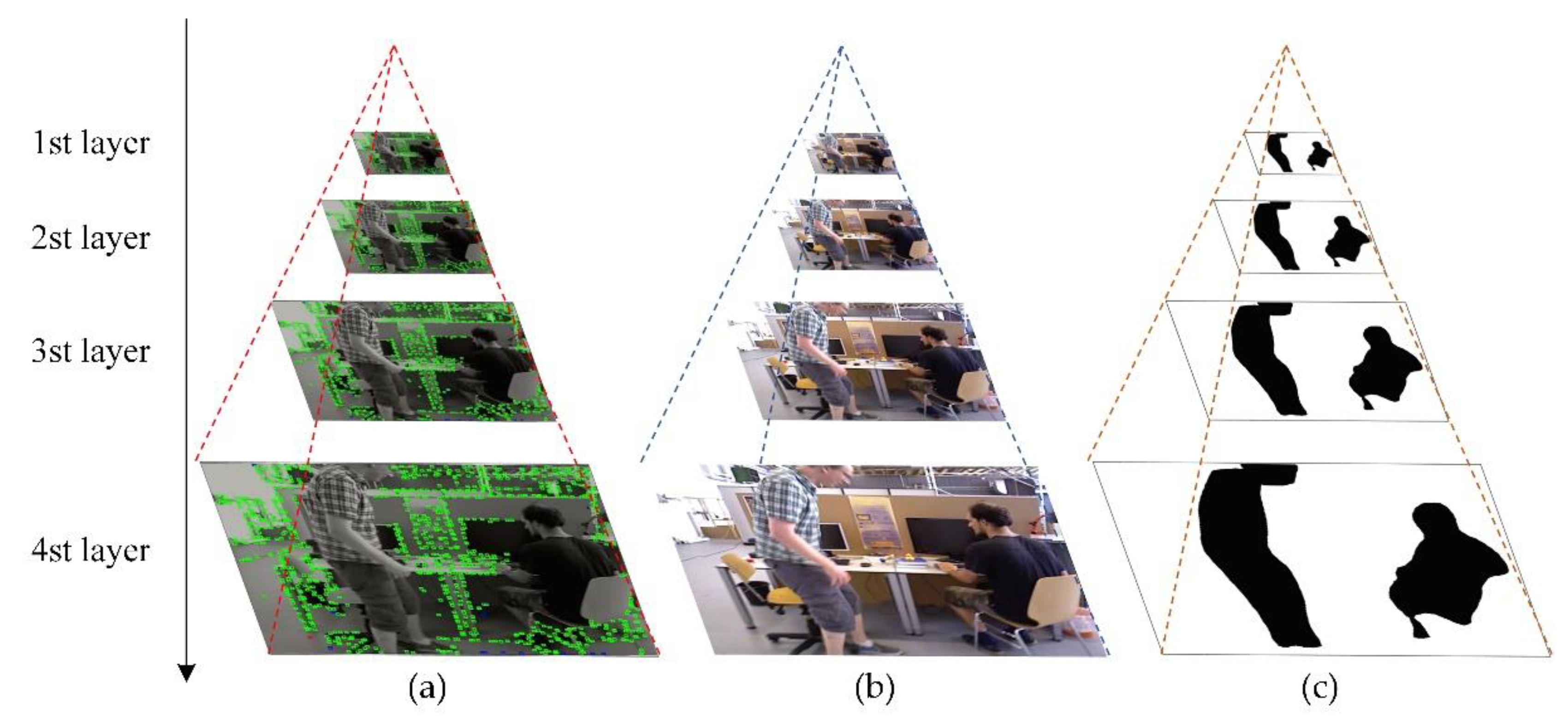
4.2. Pyramid Motion Tracking Model Based on Image Semantic Information

The image pyramid is composed of images with different resolutions, obtained by scaling the original image. Taking the original image as the bottom of the pyramid, the image of the upper layer is obtained by scaling the image of the lower layer at a certain rate.
When solving the camera pose by minimizing the photometric error, the optimization is started from the top layer of the pyramid, and then the optimization result of the previous layer is used as the initial value of the optimization of the next layer. Due to the upper layer image being relatively coarse, this process is called the coarse-to-fine strategy. Direct visual odometry requires the camera motion between two adjacent frames to be as small as possible, which avoids encountering a local minimum during optimization. The advantage of using the image pyramid is that when the motion between two adjacent frames is large, the pixel motion is still in a small range in the top image of pyramid, which is shown in Figure 4.
According to Section 4.1, when the candidate points are extracted from the keyframe, points in dynamic region are removed. However, when the candidate points in the keyframe are projected to the subsequent frame for photometric error calculation, due to the changing relative pose in the optimization process and occlusion caused by dynamic objects, candidate points in static region of keyframe may still be projected to the dynamic region of the subsequent frame, thus affecting the optimization process. Our basic idea is to remove the photometric error calculated by the projection points in a dynamic region. As shown in Figure 5. These residuals will not participate in the solution of the optimization equation.
For the keyframe, the image pyramid is constructed with the scale factor 0.5. According to Section 4.1, candidate points are extracted from the image of each pyramid layer, as shown in Figure 6a. For the subsequent frame, the same pyramid model is constructed (Figure 6b), and the semantic image of each layer containing the prior information of dynamic objects is obtained, as shown in Figure 6c.
Taking the k-th layer of the pyramid model as example, for a candidate point p in keyframe I i k , the photometric error E p j k generated by projecting p onto subsequent frame I j k can be described follows:
E p j k = p N p w p ( I j k [ p ] b j ) t j e a j t i e a i ( I i k [ p ] b i ) γ
where I i k and I j k are images of I i and I j at the k-th pyramid layer, p is the projection of point p on I j k , t i and t j are the exposure time for I i and I j , . γ represents the Huber norm, a i , a j , b i , b j are brightness transfer function parameters, N p is the residual pattern with eight surrounding neighbors and w p represents the weighting factor.
For each candidate point p in I i k , a label C p j k is calculated according to the position of the projection point p to determine whether the corresponding residual is removed or not:
C p j k = I j s e m k ( p )
where I j s e m k is the binary semantic image of I j k . In the binary semantic image, the pixel color of the dynamic region is black, and the pixel value is 0, and the pixel color of the static region is white with the value 1.
Accumulate the projection residuals of all candidate points in I i k :
E p h o t o k = p P i k C p j k E p j k
where P i k is the set of candidate points in I i k .
The relative pose between frame I i and I j can be obtained by applying Gauss–Newton method to optimize E p h o t o k . The optimization result of the k-th pyramid layer is used as the initial value of the k + 1-th pyramid layer optimization, until the optimization of the bottom pyramid layer is completed.

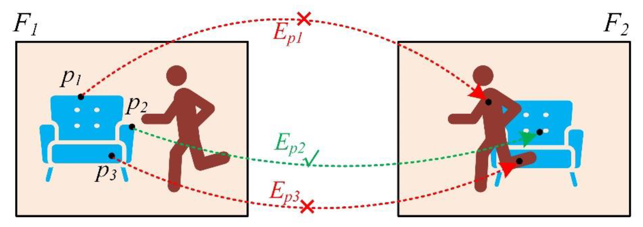
4.3. Candidate Point Tracking Based on Image Semantic Information

After the relative pose between the keyframe and the subsequent frame is obtained, the candidate points in the keyframe are tracked in the subsequent frame. Epipolar search and optimization of photometric error are adopted to find the best matching position in the subsequent frame for a candidate point in the keyframe, and inverse depth of this point is updated.
Due to the occlusion and repetitive areas, there will be mismatches, outlier and occlusion detection is required. Two traditional rules are applied to handle with it. Firstly, points for which the minimum of is not sufficiently distinct are discarded when doing the epipolar search. Secondly, point observations for which the photometric error E p j calculated by Equation (2) exceeds a threshold are removed.
In addition to the above two traditional rules, we take the semantic information of dynamic objects in the image into account. Candidate points in the keyframe for which the best matching position is in dynamic regions of the subsequent frame are considered as outlier.

4.4. Sliding Window Optimization Based on Image Semantic Information

For a single point p in keyframe I i , its projection to another keyframe I j in the sliding window is p , and the photometric error between p and p is defined by Equation (2).
Similar to Section 4.2, we define a label for each point to eliminate the residual formed by the point projected in the dynamic region:
C p j = I j s e m ( p )
where I j s e m is the binary semantic image of keyframe I j .
The full photometric error over all keyframes in the sliding window and points is given by:
E p h o t o = i F p P i j o b s ( p ) C p j E p j
where F represents the set of all keyframes in the sliding window, P i is the set of all the points in keyframe I i , and o b s ( p ) is the set of the keyframes where the point p is visible.
The pose of each keyfame and depth of each selected point can be obtained by applying Gauss-Newton method to E p h o t o .

5. Experiment and Analysis

In order to verify the positioning accuracy and robustness of the proposed method, we carry out experiments in the public TUM dataset [29], Euroc dataset [30] and dataset collected by ourselves. It is worth noting that there are few public available high dynamic datasets with pose groundtruth. Therefore, we synthesize three dynamic image sequences based on Euroc dataset. Euroc dataset is collected in a static scene, we consider dynamic objects as noise which is added into images in Euroc dataset artificially. After adding dynamic objects, the Euroc dataset is changed from a static scene to a dynamic scene, which can be used to evaluate the performance of Dynamic-DSO in high dynamic environments. Dynamic-DSO is based on the direct method. In order to show the effectiveness and superiority of the proposed system, we compare it with DSO, which is the state of art in direct methods.
In Section 5.1, the TUM dynamic dataset is used to compare the candidate points extraction between Dynamic-DSO and DSO in high dynamic environments. In Section 5.2, We use TUM dynamic dataset, the modified Euroc dataset and the self-collected image sequence to evaluate the positioning performance of Dynamic-DSO in dynamic scenes. In Section 5.3, the comparison of semi-dense point cloud maps of Dynamic-DSO and DSO is conducted.
All experiments are conducted on a workstation equipped with an Intel Xeon E5-2690v4 CPU (14 cores, 2.6GHz), 128GB memory and an NVIDIA Titan V GPU with 12GB video memory. The operating system version is Ubuntu 16.04.5 LTS.

5.1. Evaluation of Candidate Point Extraction

The TUM RGB-D dataset [29] contains several dynamic image sequences with an image collection frequency of 30Hz and resolution of 640 × 480. Each image matches the high-precision pose groundtruth provided by the motion capture system. For the traditional direct visual odometry based on the assumption of static environment, the dynamic objects in the scene will affect the final positioning results.
Figure 7 shows the comparison of Dynamic-DSO and DSO for extracting candidate points in keyframes. Two pedestrians walk around in front of the camera. The candidate points extracted by DSO (Figure 7c) include pedestrians. The proposed method segments dynamic pedestrians (Figure 7b) and only extracts candidate points from the static area (Figure 7d), which ensures that interference from dynamic objects is avoided when calculating photometric error.

5.2. Evaluation of Position Performance

5.2.1. Evaluation on the Public TUM Dynamic Dataset

Three dynamic sequences including fr3_walking_xyz, fr3_walking_rpy, and fr3_walking_halfsphere in TUM dataset are used to evaluate the positioning result of Dynamic-DSO. In the three sequences, two pedestrians walk around the table quickly in front of the camera, which is the typical indoor high dynamic scene and has high requirements for the robustness of the direct visual odometry.
DSO cannot complete initialization in these three dynamic sequences, so it cannot give positioning results. In this paper, after removing the interference of dynamic objects by combining the image semantic segmentation, Dynamic-DSO can initialize successfully in these dynamic sequences, and gives decent positioning results, which improves the practicability and robustness of visual odometry based on direct method in dynamic scenes.
Figure 8 shows the heat maps of the positioning trajectory of Dynamic-DSO in three sequences, where the gray dotted line is the trajectory groundtruth, the colorful solid line is the estimated trajectory of Dynamic-DSO. The color indicates absolute pose error (APE) for the translation part between the estimated trajectory and groundtruth. The color bar represents that the error gradually increases from the cold color to the warm color. From three heat maps, it can be seen that the trajectory estimated by Dynamic-DSO fits well with the groundtruth (note that in Figure 8b, due to the small motion amplitude of camera, it seems that the deviation between the estimated trajectory and the groundtruth is large, but the maximum error is only 0.129 m).
Table 1 gives statistics on the APE for the translation part of the Dynamic-DSO and DSO in three TUM fr3_walking dynamic sequences. Since the current published methods are based on indirect method (feature point method), in addition to the comparison with DSO, we also compared the proposed method with several systems based on indirect method in the public TUM dynamic dataset, including SOF-SLAM [3], DS-SLAM [14], Dynamic-SLAM [16] and Semantic SLAM [15]. It is worth noting that since our system is based on a direct method, the positioning accuracy is slightly lower than that of the systems based on the feature point method in the texture-rich dataset such as TUM dynamic dataset, which can be explained in more detail in [31]. However, as the parallel branch to the feature point method in the SLAM and VO field, the direct method has the advantages of better positioning accuracy and system robustness than the feature point method when there are not enough feature points due to the weak texture environment [1,31], and can construct the semi-dense map.
As shown in the table, due to the failed initialization, DSO which is the state of the art system of direct method, cannot output positioning results. It can be seen from the root mean square error (RMSE) that the trajectory error of Dynamic-DSO is less than 6cm by combining image semantic segmentation, which significantly improves the positioning accuracy and robustness of direct method in dynamic environment.

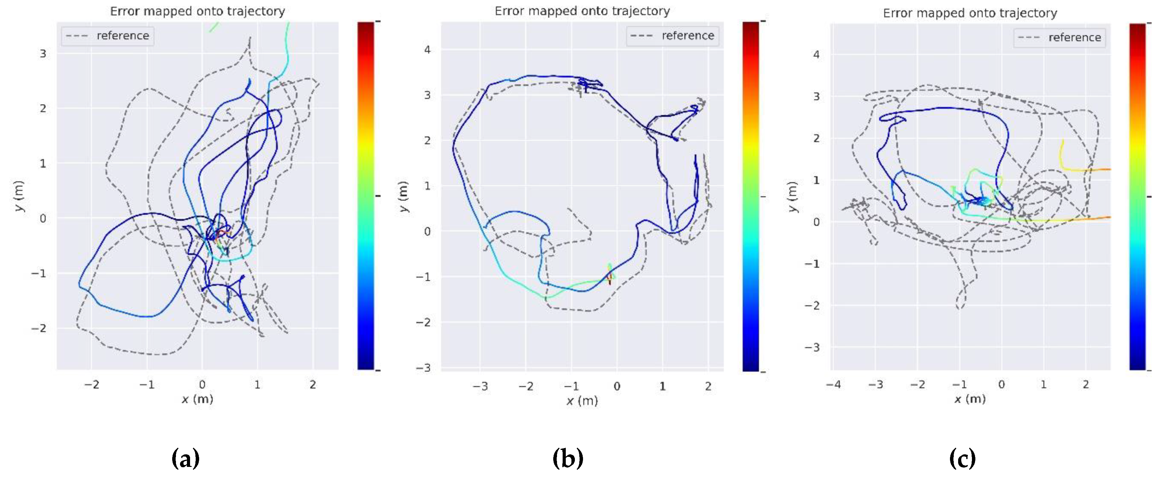
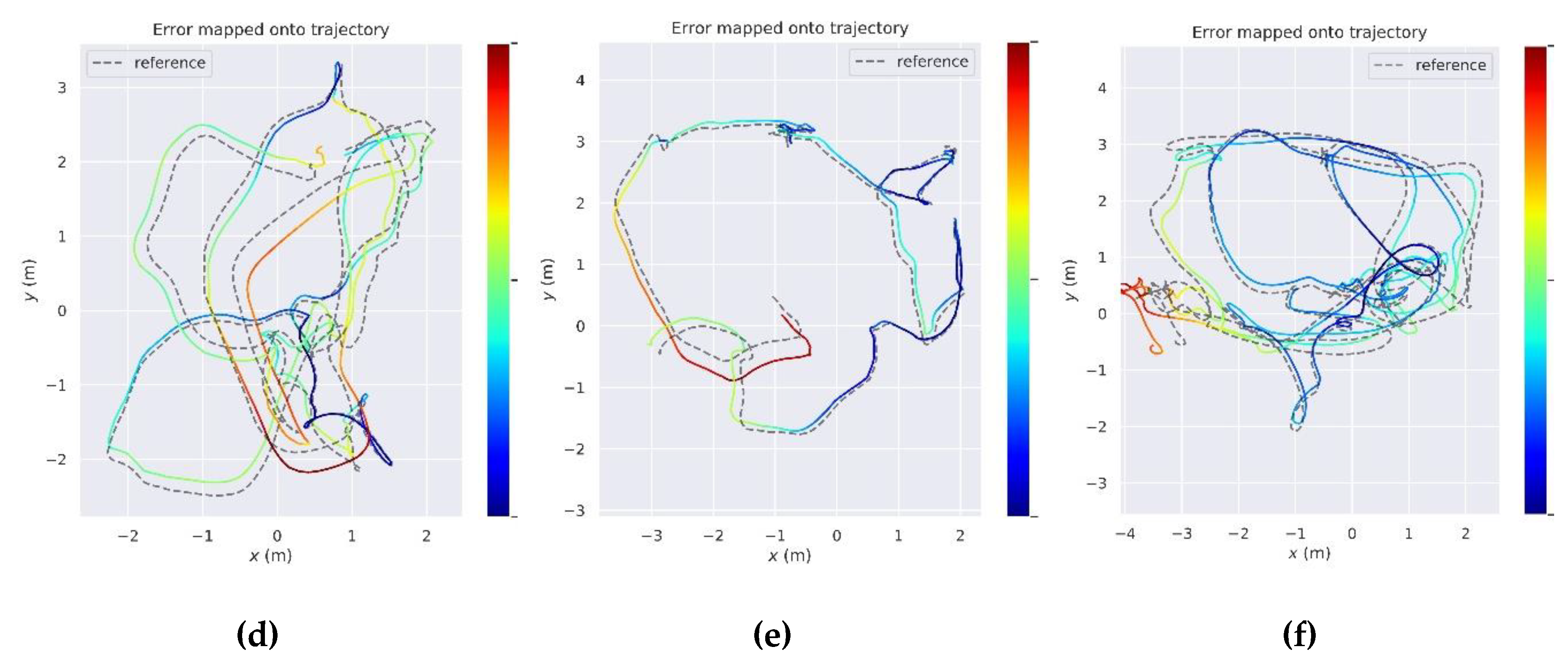
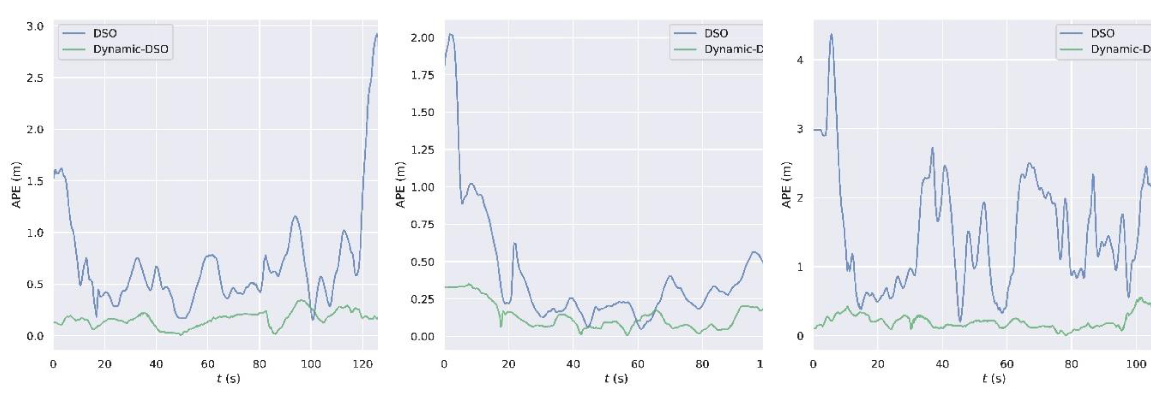
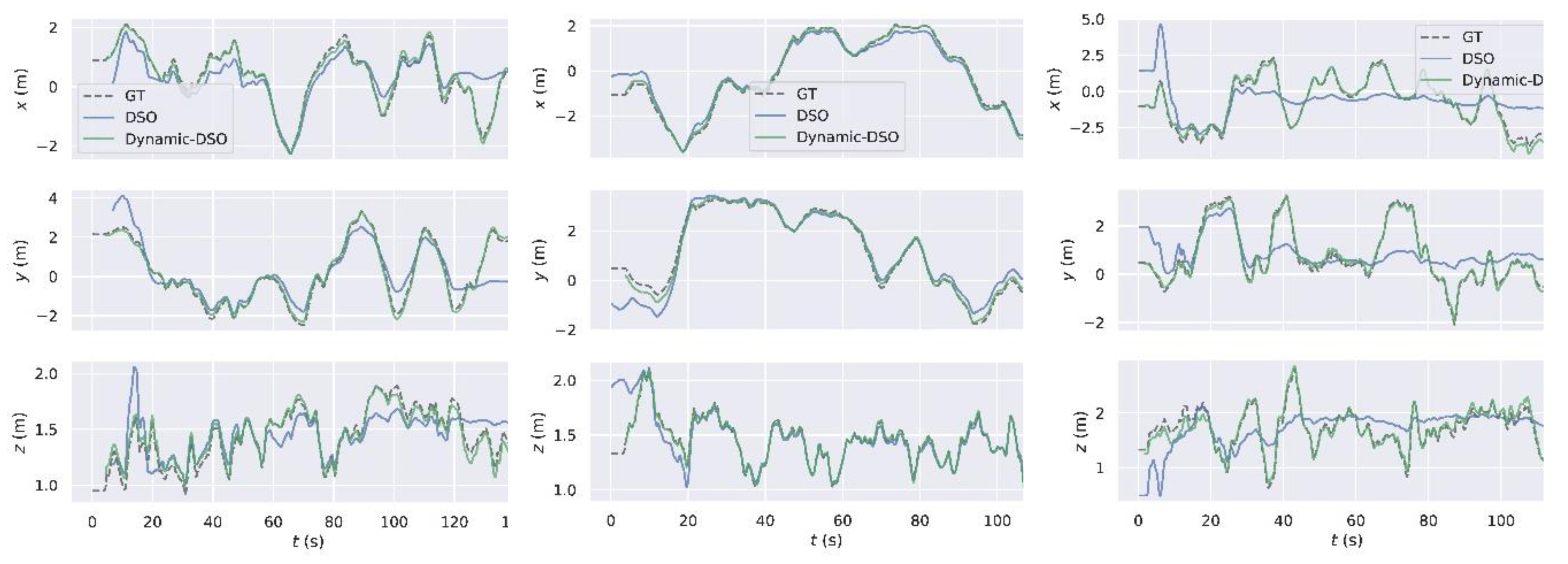
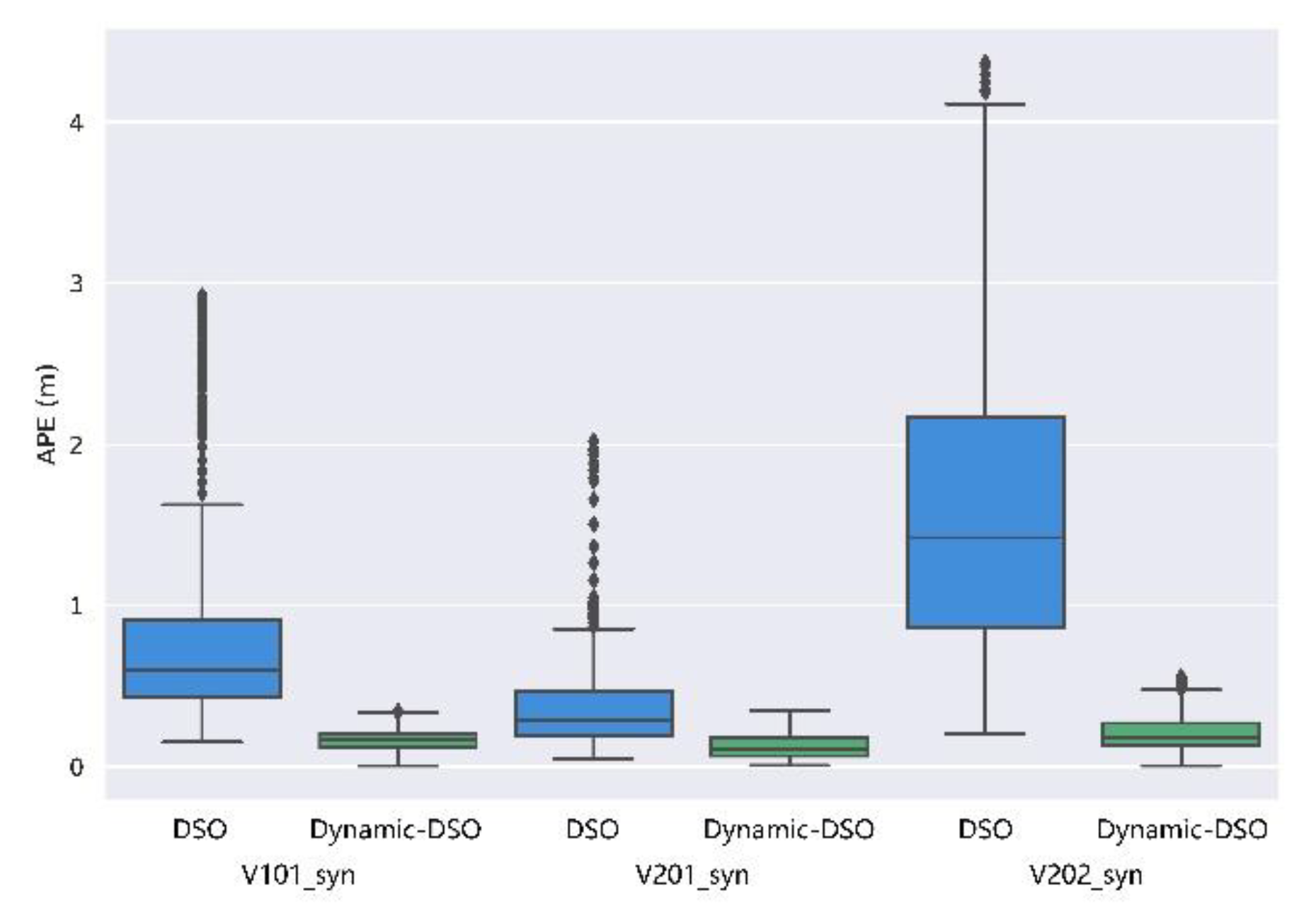
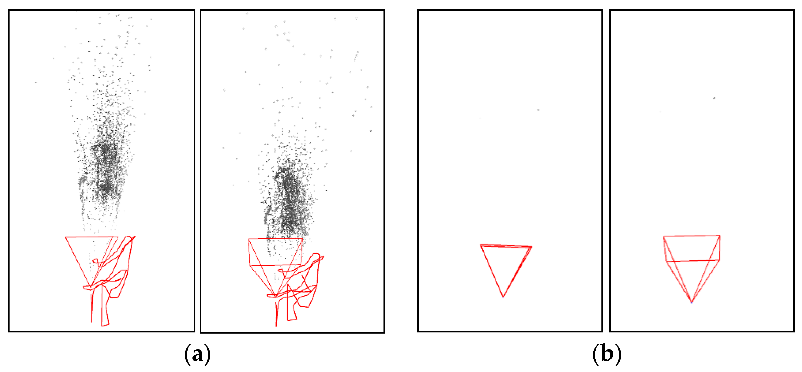
5.2.2. Evaluation on the Modified Euroc Dynamic Dataset

The existing public indoor small-scale dynamic dataset is relatively small, we have conducted the comparative experiment in the public TUM indoor dynamic dataset. To further evaluate the performance of the proposed method and DSO in the indoor small-scale dynamic scenes, we inserted dynamic objects into the static Euroc indoor dataset. In the public Euroc dataset, each image is matched with a high-precision pose groundtruth obtained from the professional optical motion capture system, so after inserting the dynamic object into Euroc dataset, we can get the dynamic image sequence matching the high-precision pose groundtruth. Then we can make quantitative analysis by comparing the estimated results with the groundtruth.
• Data Preprocessing
The Euroc dataset [30] is collected in static scene. The collection frequency is 20Hz, and the resolution is 752 × 480. Each image matches the high-precision groundtruth provided by the motion capture system. We consider moving pedestrian as the noise, which is artificially synthesized into the Euroc image sequences. The image sequences are changed from a static scene to a dynamic scene after adding dynamic objects.
As shown in Figure 9, the device that records the dynamic pedestrian video sequence is an Intel ZR300 camera containing a color global shutter camera, and a laptop with Intel Core i7-7000 CPU and 8GB memory. Firstly, we fix the acquisition device on the indoor desktop, and a person walks around as dynamic object in front of the camera. A video sequence containing the dynamic pedestrian is recorded at the same frequency and image resolution as the Euroc dataset. Then, the dynamic pedestrian in each frame is segmented by using Mask-RCNN [25]. Finally, the segmented continuous moving pedestrian is added to each image in the Euroc image sequence to synthesize the Euroc dynamic scene dataset. We add dynamic objects to the image sequences in the Euroc dataset including V1_01, V2_01 and V2_02, and record the names of these modified sequences as V101_syn, V201_syn and V202_syn. By using V101_syn, V201_syn and V202_syn, the performance of DSO and Dynamic-DSO can be evaluated in dynamic scenes.
Figure 10 shows the processing of the V202_syn sequence. Figure 10a shows images in the original V2_02 sequence. It can be seen that these images do not contain any moving objects. Figure 10b shows images collected by ourselves in the indoor environment, which contain a moving pedestrian. Mask-RCNN is used to segment the pedestrians in Figure 10b, and the result of segmentation is shown in Figure 10c. By using the semantic image as mask, the pedestrian in Figure 10b is extracted and synthesized into the V2_02 sequence in Figure 10a, which generates the synthetic V202_syn sequence shown in Figure 10d.
• Comparative Analysis of Positioning Performance
Figure 11 shows the heat maps of the positioning trajectory of DSO (Figure 11a–c) and Dynamic-DSO (Figure 11d–f) in V101_syn, V201_syn, and V202_syn respectively. From three heat maps, it can be seen that the trajectory estimated by Dynamic-DSO is closer to the groundtruth than DSO in three image sequences, and the maximum, minimum and average values of trajectory error are less than DSO.
Figure 12 compares the trajectory error with time of Dynamic-DSO and DSO in three synthetic sequences. The trajectory error of DSO exceeds 1m for quite a long time and the fluctuation is obvious. The maximum error in the V202_syn sequence exceeds 4 m, which cannot meet the accuracy requirements in indoor positioning. The trajectory error of Dynamic-DSO is much lower than DSO. The maximum value is 0.557 m in the V202_syn sequence, and the error fluctuation of the whole positioning process is small. Figure 13 shows the positioning results of DSO and Dynamic-DSO in three axes x, y, z. Compared with DSO, the positioning results of the proposed method are closer to the groundtruth in each axes in dynamic environments.
Figure 14 is the boxplot of the trajectory error between Dynamic-DSO and DSO, which is used to analyze the discrete distribution of the error. The box of Dynamic-DSO is flatter, meaning that the trajectory error of the proposed system is more concentrated. Compared to DSO, the upper and lower limiting values of Dynamic-DSO are lower, the median, the upper and lower quartiles are smaller, and the outliers are very few—verifying that the positioning accuracy and robustness of Dynamic-DSO are more superior than those of DSO in three dynamic sequences.
Table 2 shows statistics for the trajectory error of the DSO and Dynamic-DSO in V101_syn, V201_syn and V202_syn. Comparing the RMSE of the two methods, the positioning accuracy of the proposed method in the dynamic environment is significantly higher than that of DSO.

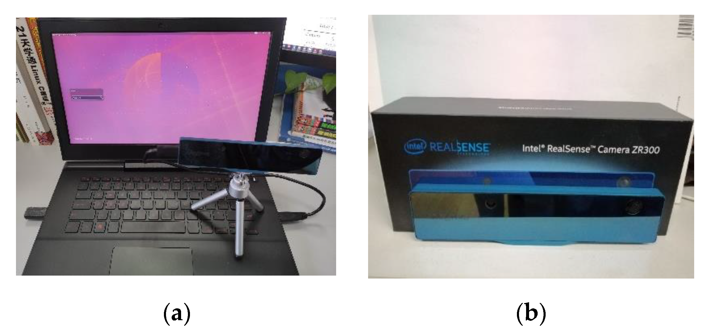
5.2.3. Evaluation on the Self-Collected Sequence

In Section 5.2.2, in order to add dynamic objects to the original Euroc dataset, we fix the camera in an indoor environment and record a sequence, including a pedestrian walking in front of the camera. In this section, we will use this sequence to evaluate the performance of Dynamic-DSO and DSO in the actual dynamic environment by comparing the point cloud maps and camera trajectories.
The camera trajectories and point cloud maps estimated by Dynamic-DSO and DSO are shown in Figure 15. Although the camera remains stationary, there is relative motion between the pedestrian and the camera. As shown in Figure 15a, DSO is cheated by the dynamic pedestrian, which leads to the wrong judgment of the camera state and the large drift of the estimated trajectory. Compared with DSO, the camera trajectory estimated by Dynamic-DSO is almost at a point without large-scale drift after suppressing the interference of the pedestrian.
In order to further explain the impact of dynamic object on algorithm, some keyframes selected during the algorithm running are shown in Figure 16. As shown in Figure 16a, due to the interference of dynamic objects, most of the points that DSO chooses to track fall on the dynamic pedestrian. Although the camera is fixed on the desktop, DSO mistakenly judges that the camera is moving due to the relative motion between the camera and the pedestrian. In contrast, Dynamic-DSO successfully detects the position of the pedestrian and selects points in static region to track.

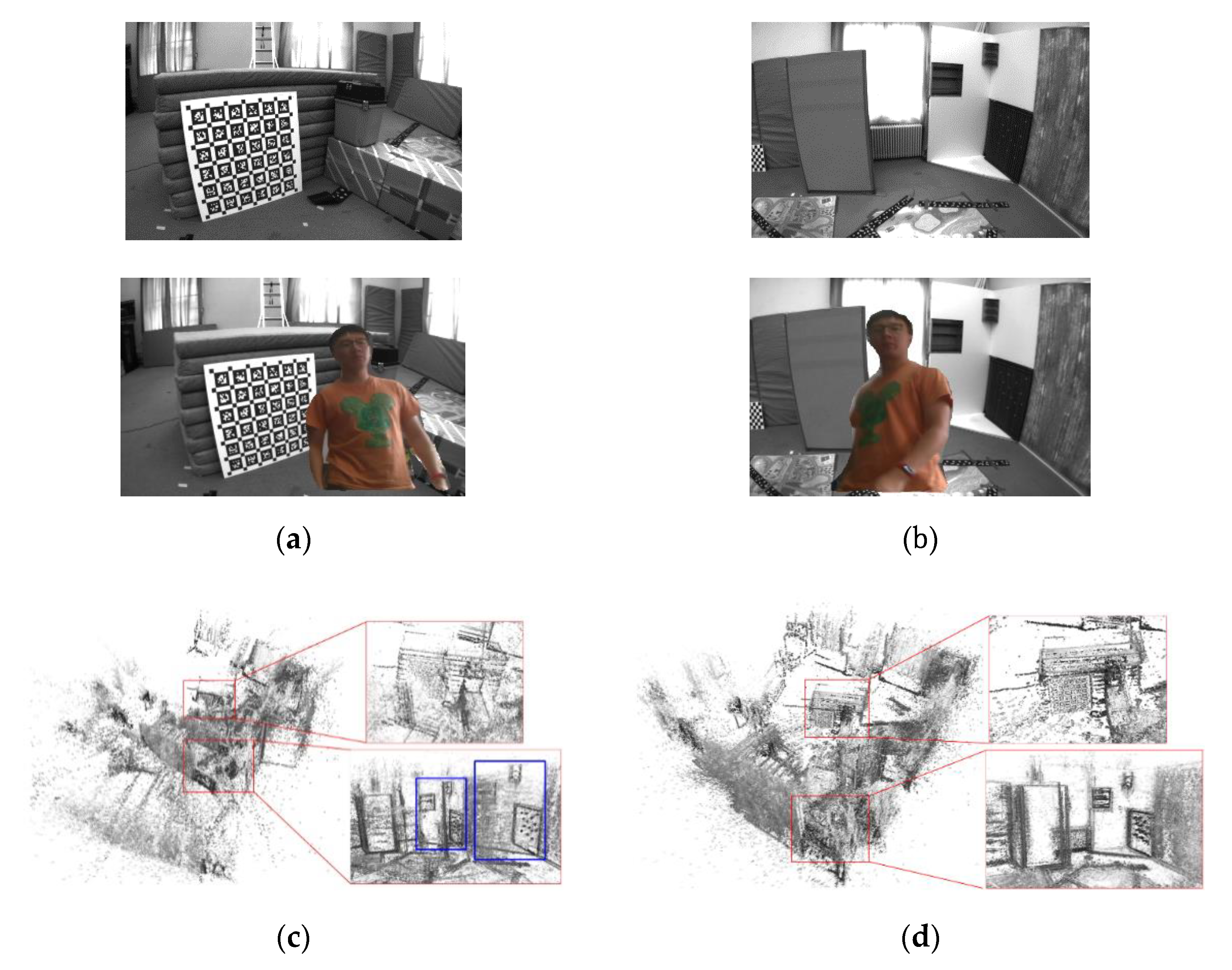
5.3. Evaluation of Mapping Performance

Figure 17 shows the 3D point cloud map of indoor scene constructed by Dynamic-DSO and DSO in V101_syn sequence and the partial enlarged map of the calibration board and the room corner. The map of DSO (Figure 17c) is obviously disturbed by the pedestrian, the map is unclear, and the overall position and part of the structure show serious ghosting and drift. Comparing the enlarged calibration board maps of Dynamic-DSO and DSO (upper right of Figure 17c,d), the map constructed by Dynamic-DSO, which removes the interference of dynamic objects, has clearer outlines and richer details than DSO. The room corner maps constructed by Dynamic-DSO and DSO are shown in the bottom right of Figure 17c,d. The map of DSO obviously has drift and ghosting, that is, the contents of the two blue boxes in the bottom right of Figure 17c should coincide with each other. In Figure 17d, the drift and ghosting do not appear.

6. Conclusions

In this paper, Dynamic-DSO is proposed, which is a semantic monocular direct visual odometry using image semantic segmentation method in deep learning to improve the performance of positioning and mapping in dynamic environments. This is different from the most current systems, which combine the traditional indirect SLAM or VO with deep learning. The proposed system is completed based on direct method. Firstly, image semantic segmentation technology is used to obtain the pixel-wise semantic information of the dynamic objects in images. Secondly, a novel candidate points extraction method and a tracking model are proposed to eliminate the dynamic objects in an effective way by using the image semantic information. Finally, we apply the semantic information of dynamic objects into the sliding window optimization to avoid dynamic objects disturbing the optimization process. The proposed method was evaluated both on the public TUM dynamic dataset and the modified Euroc dynamic dataset, and we compared the pose estimation performance of our method with the state-of-the-art direct method. The results demonstrate the accuracy and robustness of the proposed method. The position accuracy of Dynamic-DSO is significantly higher than the state-of-the-art direct method in dynamic environments, and the semi-dense cloud map constructed by Dynamic-DSO is clearer and more detailed. In the future, a more real-time semantic segmentation framework should be used to improve the real-time performance of the entire system. Considering the semantic information and the Sparse-to-Dense model proposed by Ma et al. [32], we might build a dense 3D semantic map in dynamic environments based on the semi-dense map constructed by Dynamic-DSO.

Author Contributions

Conceptualization, C.S. and S.P.; methodology, C.S.; software, C.S. and Y.T.; validation, C.S., S.P. and W.G.; formal analysis, Y.T. and T.Z.; investigation, C.S. and Y.T.; resources, W.G.; data curation, T.Z.; writing—original draft preparation, C.S.; writing—review and editing, C.S. and S.P.; supervision, S.P.; project administration, S.P. and W.G.; funding acquisition, S.P. All authors have read and agreed to the published version of the manuscript.

Funding

This work is partially supported by the National Natural Science Foundation of China (Grant No. 41774027, Grant No. 41904022 and Grant No. 41574026) and the National Key Technologies R&D Program (Grant No. 2016YFB0502101).

Conflicts of Interest

The authors declare no conflict of interest.

References

  1. Gu, Z.; Liu, H. A survey of monocular simultaneous localization and mapping. CAAI Trans. Intell. Syst. 2015, 10, 499–507. [Google Scholar]
  2. Guo, R.; Peng, K.; Fan, W.; Zhai, Y.; Liu, Y. RGB-D SLAM Using Point–Plane Constraints for Indoor Environments. Sensors 2019, 19, 2721. [Google Scholar] [CrossRef] [PubMed] [Green Version]
  3. Cui, L.; Ma, C. SOF-SLAM: A semantic visual SLAM for Dynamic Environments. IEEE Access 2019, 7, 166528–166539. [Google Scholar] [CrossRef]
  4. Yousif, K.; Bab-Hadiashar, A.; Hoseinnezhad, R. An overview to visual odometry and visual SLAM: Applications to mobile robotics. Intell. Ind. Syst. 2015, 1, 289–311. [Google Scholar] [CrossRef]
  5. Cadena, C.; Carlone, L.; Carrillo, H.; Latif, Y.; Scaramuzza, D.; Neira, J.; Reid, I.; Leonard, J.J. Past, present, and future of simultaneous localization and mapping: Toward the robust-perception age. IEEE Trans. Robot. 2016, 32, 1309–1332. [Google Scholar] [CrossRef] [Green Version]
  6. Davison, A.J.; Reid, I.D.; Molton, N.D.; Stasse, O. MonoSLAM: Real-time single camera SLAM. IEEE Trans. Pattern Anal. Mach. Intell. 2007, 29, 1052–1067. [Google Scholar] [CrossRef] [PubMed] [Green Version]
  7. Klein, G.; Murray, D. Parallel tracking and mapping for small AR workspaces. In Proceedings of the 2007 6th IEEE and ACM International Symposium on Mixed and Augmented Reality, Nara, Japan, 13–16 November 2007; pp. 1–10. [Google Scholar]
  8. Mur-Artal, R.; Tardós, J.D. Orb-slam2: An open-source slam system for monocular, stereo, and rgb-d cameras. IEEE Trans. Robot. 2017, 33, 1255–1262. [Google Scholar] [CrossRef] [Green Version]
  9. Engel, J.; Schöps, T.; Cremers, D. LSD-SLAM: Large-scale direct monocular SLAM. In Proceedings of the European Conference on Computer Vision, Zurich, Switzerland, 6–12 September 2014; pp. 834–849. [Google Scholar]
  10. Forster, C.; Pizzoli, M.; Scaramuzza, D. SVO: Fast semi-direct monocular visual odometry. In Proceedings of the 2014 IEEE International Conference on Robotics and Automation (ICRA), Hong Kong, China, 31 May–7 June 2014; pp. 15–22. [Google Scholar]
  11. Engel, J.; Koltun, V.; Cremers, D. Direct sparse odometry. IEEE Trans. Pattern Anal. Mach. Intell. 2017, 40, 611–625. [Google Scholar] [CrossRef] [PubMed]
  12. Chen, W.; Fang, M.; Liu, Y.-H.; Li, L. Monocular semantic SLAM in dynamic street scene based on multiple object tracking. In Proceedings of the 2017 IEEE International Conference on Cybernetics and Intelligent Systems (CIS) and IEEE Conference on Robotics, Automation and Mechatronics (RAM), Ningbo, China, 19–21 November 2017; pp. 599–604. [Google Scholar]
  13. Bescos, B.; Fácil, J.M.; Civera, J.; Neira, J. DynaSLAM: Tracking, mapping, and inpainting in dynamic scenes. IEEE Robot. Autom. Lett. 2018, 3, 4076–4083. [Google Scholar] [CrossRef] [Green Version]
  14. Yu, C.; Liu, Z.; Liu, X.-J.; Xie, F.; Yang, Y.; Wei, Q.; Fei, Q. Ds-slam: A semantic visual slam towards dynamic environments. In Proceedings of the 2018 IEEE/RSJ International Conference on Intelligent Robots and Systems (IROS), Madrid, Spain, 1–5 October 2018; pp. 1168–1174. [Google Scholar]
  15. Zhang, L.; Wei, L.; Shen, P.; Wei, W.; Zhu, G.; Song, J. Semantic SLAM Based on Object Detection and Improved Octomap. IEEE Access 2018, 6, 75545–75559. [Google Scholar] [CrossRef]
  16. Xiao, L.H.; Wang, J.G.; Qiu, X.S.; Rong, Z.; Zou, X.D. Dynamic-SLAM: Semantic monocular visual localization and mapping based on deep learning in dynamic environment. Robot. Auton. Syst. 2019, 117, 1–16. [Google Scholar] [CrossRef]
  17. Bibby, C.; Reid, I. Simultaneous localisation and mapping in dynamic environments (SLAMIDE) with reversible data association. Proc. Robot. Sci. Syst. 2007, 66, 81. [Google Scholar]
  18. Walcott-Bryant, A.; Kaess, M.; Johannsson, H.; Leonard, J.J. Dynamic pose graph SLAM: Long-term mapping in low dynamic environments. In Proceedings of the 2012 IEEE/RSJ International Conference on Intelligent Robots and Systems, Vilamoura, Portugal, 7–12 October 2012; pp. 1871–1878. [Google Scholar]
  19. Zou, D.; Tan, P. Coslam: Collaborative visual slam in dynamic environments. IEEE Trans. Pattern Anal. Mach. Intell. 2012, 35, 354–366. [Google Scholar] [CrossRef] [PubMed]
  20. Kerl, C.; Sturm, J.; Cremers, D. Robust odometry estimation for RGB-D cameras. In Proceedings of the 2013 IEEE International Conference on Robotics and Automation, Karlsruhe, Germany, 6–10 May 2013; pp. 3748–3754. [Google Scholar]
  21. Bakkay, M.C.; Arafa, M.; Zagrouba, E. Dense 3D SLAM in dynamic scenes using Kinect. In Proceedings of the Iberian Conference on Pattern Recognition and Image Analysis, Santiago de Compostela, Spain, 17–19 June 2015; pp. 121–129. [Google Scholar]
  22. Li, S.; Lee, D. RGB-D SLAM in dynamic environments using static point weighting. IEEE Robot. Autom. Lett. 2017, 2, 2263–2270. [Google Scholar] [CrossRef]
  23. Bahraini, M.S.; Bozorg, M.; Rad, A.B. SLAM in dynamic environments via ML-RANSAC. Mechatronics 2018, 49, 105–118. [Google Scholar] [CrossRef]
  24. Redmon, J.; Farhadi, A. YOLO9000: Better, faster, stronger. In Proceedings of the IEEE Conference on Computer Vision and Pattern Recognition, Honolulu, HI, USA, 21–26 July 2017; pp. 7263–7271. [Google Scholar]
  25. He, K.; Gkioxari, G.; Dollár, P.; Girshick, R. Mask r-cnn. In Proceedings of the IEEE International Conference on Computer Vision, Venice, Italy, 22–29 October 2017; pp. 2961–2969. [Google Scholar]
  26. Badrinarayanan, V.; Kendall, A.; Cipolla, R. Segnet: A deep convolutional encoder-decoder architecture for image segmentation. IEEE Trans. Pattern Anal. Mach. Intell. 2017, 39, 2481–2495. [Google Scholar] [CrossRef] [PubMed]
  27. Liu, W.; Anguelov, D.; Erhan, D.; Szegedy, C.; Reed, S.; Fu, C.-Y.; Berg, A.C. Ssd: Single shot multibox detector. In Proceedings of the European Conference on Computer Vision, Amsterdam, The Netherlands, 8–16 October 2016; pp. 21–37. [Google Scholar]
  28. Mask R-CNN for Object Detection and Instance Segmentation on Keras and TensorFlow. Available online: https://github.com/matterport/Mask_RCNN (accessed on 15 October 2019).
  29. Sturm, J.; Engelhard, N.; Endres, F.; Burgard, W.; Cremers, D. A benchmark for the evaluation of RGB-D SLAM systems. In Proceedings of the 2012 IEEE/RSJ International Conference on Intelligent Robots and Systems, Vilamoura, Portugal, 7–12 October 2012; pp. 573–580. [Google Scholar]
  30. Burri, M.; Nikolic, J.; Gohl, P.; Schneider, T.; Rehder, J.; Omari, S.; Achtelik, M.W.; Siegwart, R. The EuRoC micro aerial vehicle datasets. Int. J. Robot. Res. 2016, 35, 1157–1163. [Google Scholar] [CrossRef]
  31. Mur-Artal, R.; Montiel, J.M.M.; Tardos, J.D. ORB-SLAM: A versatile and accurate monocular SLAM system. IEEE Trans. Robot. 2015, 31, 1147–1163. [Google Scholar] [CrossRef] [Green Version]
  32. Mal, F.; Karaman, S. Sparse-to-dense: Depth prediction from sparse depth samples and a single image. In Proceedings of the 2018 IEEE International Conference on Robotics and Automation (ICRA), Brisbane, Australia, 21–25 May 2018; pp. 1–8. [Google Scholar]
Figure 1. Framework of Dynamic-DSO (Direct Sparse Odometry), color parts and the content in the dotted box show our contributions.
Applsci 10 01467 g001
Figure 2. Based on life experience, the dynamic degree of common objects is scored. Only a few common objects are listed. The threshold is set to 5. If the detection score of an object is higher than the threshold, it is considered as a dynamic object, otherwise we think it as a static object.
Applsci 10 01467 g002
Figure 3. The upper line is the RGB images in TUM dynamic dataset [29], and the bottom line is the indoor pedestrians segmentation results by Mask R-CNN, where the black parts are dynamic regions. The pixel value of black regions (dynamic regions) is 0. The pixel value of white regions (static regions) is 1.
Applsci 10 01467 g003
Figure 4. Assuming that the original image resolution is 6 × 8 (row × column), the pixels projected from P to the two frames F1 and F2 are p1 and p2, and the distance between p1 and p2 is 4 pixels. The original image is scaled with a 0.5 scaling factor, and the scaled image size is 3 × 4, the distance between the two projection points p1′ and p2′ is reduced to 2 pixels. The size of an actual image is much larger, and the image in the top layer of the pyramid can limit the pixel motion to a small range.
Applsci 10 01467 g004
Figure 5. F1 is a keyframe. p1, p2 and p3 are candidate points extracted according to Section 4.1. F2 is the subsequent frame of F1. Three points are projected to F2 to form three residuals. If the projection point falls in the dynamic region of F2, the corresponding residual will be removed.
Applsci 10 01467 g005
Figure 6. (a,b) show the image pyramids constructed by the keyframe and subsequent frame. (c) shows the semantic image of each layer in subsequent frame pyramid.
Applsci 10 01467 g006
Figure 7. Comparison of Dynamic-DSO and DSO for extracting candidate points in keyframes. (a): Keyframes containing dynamic objects. (b): Semantic images containing dynamic objects obtained by Dynamic-DSO. (c): Candidate points extracted by DSO. (d): Candidate points extracted by Dynamic-DSO.
Applsci 10 01467 g007
Figure 8. Heat maps of the positioning trajectory of Dynamic-DSO in three sequences. (a): The estimated trajectory heat map on fr3_walking_xyz. (b): The estimated trajectory heat map on fr3_walking_rpy. (c): The estimated trajectory heat map on fr3_walking_halfsphere. DSO cannot complete initialization in these three dynamic sequences, so it cannot give positioning results.
Applsci 10 01467 g008
Figure 9. The acquisition equipment includes a laptop (a) and an Intel zr300 camera (b), which are fixed on the desktop.
Applsci 10 01467 g009
Figure 10. The processing of the V202_syn sequence. (a): Images in original Euroc V2_02 sequence. (b): Images collected by ourselves, containing a pedestrian. (c): Sematic images obtained by Mask-RCNN. (d): Images in the modified V202_syn sequence.
Applsci 10 01467 g010
Figure 11. Heat maps of the positioning trajectory of Dynamic-DSO and DSO in three sequences. (a), (b), (c): Positioning results of DSO in V101_syn, V201_syn and V202_syn respectively. (d), (e), (f): Positioning results of Dynamic-DSO in V101_syn, V201_syn and V202_syn respectively.
Applsci 10 01467 g011aApplsci 10 01467 g011b
Figure 12. Comparison of the trajectory error with time between Dynamic-DSO and DSO in three synthetic sequences. Comparison in V101_syn, V201_syn and V202_syn is shown from left to right.
Applsci 10 01467 g012
Figure 13. Positioning results comparison of DSO and Dynamic-DSO in three axes x, y, z. GT means the groundtruth. Comparison in V101_syn, V201_syn and V202_syn is shown from left to right.
Applsci 10 01467 g013
Figure 14. Boxplot of the trajectory error between Dynamic-DSO and DSO in V101_syn, V201_syn and V202_syn.
Applsci 10 01467 g014
Figure 15. The camera trajectories and point cloud maps estimated by Dynamic-DSO (a) and DSO (b). The red triangle represents the camera orientation, the red curve is the estimated camera trajectory and the black area is the 3D point cloud map.
Applsci 10 01467 g015
Figure 16. Keyframes selected by DSO (a) and Dynamic-DSO (b). The colorful points are selected and tracked by the algorithm, and the color represents the depth information.
Applsci 10 01467 g016
Figure 17. 3D point cloud maps of indoor scene and partial enlarged maps constructed by Dynamic-DSO and DSO in V101_syn sequence. (a): Calibration board shown in V1_01 and V101_syn. (b): Room corner shown in V1_01 and V101_syn. (c): point cloud map constructed by DSO. (d): point cloud map constructed by Dynamic-DSO.
Applsci 10 01467 g017
Table 1. Comparison of absolute Pose Error (APE) for translation part in public TUM dynamic dataset. (Unit: m).
High Dynamic SequenceDynamic-SLAM [16]SOF-SLAM [3]DS-SLAM [14]Semantic SLAM [15]DSO [11]Dynamic-DSO
RmseRmseRmseRmseRmseMeanStdRmseMeanStd
fr3_walking_xyz0.0130.0180.0250.034\\\0.0320.0330.011
fr3_walking_rpy0.0600.0270.444-\\\0.0610.0620.034
fr3_walking_half0.0210.0290.0300.064\\\0.0630.0550.042
“\” means initialization failed. ‘’-’’ denotes no available data.
Table 2. Comparison of Absolute Pose Error (APE) for translation part in modified Euroc dataset. (Unit: m).
High Dynamic
Sequence
DSODynamic-DSORmse
Improvement
RmseMeanStdRmseMeanStd
V101_syn1.060.830.650.170.160.0784%
V201_syn0.510.390.340.150.130.0871%
V202_syn1.721.520.810.240.210.1186%

