Robust Estimation of Vehicle Motion States Utilizing an Extended Set-Membership Filter

Abstract

Reliable vehicle motion states are critical for the precise control performed by vehicle active safety systems. This paper investigates a robust estimation strategy for vehicle motion states by feat of the application of the extended set-membership filter (ESMF). In this strategy, a system noise source is only limited as unknown but bounded, rather than the Gaussian white noise claimed in the stochastic filtering algorithms, such as the unscented Kalman filter (UKF). Moreover, as one part of this strategy, a calculation scheme with simple structure is proposed to acquire the longitudinal and lateral tire forces with acceptable accuracy. Numerical tests are carried out to verify the performance of the proposed strategy. The results indicate that as compared with the UKF-based one, it not only has higher accuracy, but also can provide a 100% hard boundary which contains the real values of the vehicle states, including the vehicle’s longitudinal velocity, lateral velocity, and sideslip angle. Therefore, the ESMF-based strategy can proffer a more guaranteed estimation with robustness for practical vehicle active safety control.

1. Introduction

In the vehicle moving process, the accurate acquisition of motion state information is one of the key factors for the effective control of a vehicle active safety system [1,2,3]. However, the direct measurement of the vehicle motion states, including the longitudinal velocity, lateral velocity and sideslip angle, requires the help of some expensive and specialized sensors. For example, the measurement of vehicle sideslip angle can only be realized by means of a non-contact optical sensor (such as the S-Motion produced by Corrsys-Datron) [4]. Because of high cost and special installation requirements, it is difficult to apply this kind of sensors in production vehicles. On the other hand, vehicle motion states can also be determined via the soft-sensing theory which combines the linear/nonlinear filtering algorithms with the information obtained by ordinary vehicle sensors. In recent years, utilizing the soft-sensing theory including the Kalman filter (KF) to acquire vehicle motion states has become a research hotspot due to low cost and easy migratability.

Many scholars have investigated the strategies for vehicle state estimation based on the KF and its improved algorithms [5,6,7,8,9,10]. Gadola et al. [11] combined the extended Kalman filter (EKF) with a 2-degree-of-freedom (2-DOF) single-track vehicle model and the simplified Magic formula tire model to obtain the sideslip angle. Considering the influence of the vehicle parameters on estimation results, Wenzel et al. [12] designed a dual extended Kalman filter (DEKF) structure, where a parallel loop was constructed between the vehicle parameter and state estimators to acquire high-accuracy and simultaneous determination. Moreover, to alleviate the adverse impact caused by the truncation error existed in the EKF, a series of sigma-point Kalman filters were utilized for the acquirement of vehicle information, such as the unscented Kalman filter (UKF) [13,14] and the cubature Kalman filter (CKF) [15,16]. These filters draw nonlinear transformations into the framework of the KF and carry out the transformations on the sigma sampling points. On the premise that the variance and mean of these points are the same as those of the states to be estimated, the probability distributions of nonlinear functions can be approximately approached. An overview of the typical strategies for vehicle state estimation is summarized in

Table 1. Overview of the strategies for vehicle state estimation.

Filter	Vehicle Model	Tire Model	Trait	Ref.
EKF and its improvements	3-DOF dual-track	Longitudinal force observer and Magic formula	Simple estimation structure.	[6]
			Real-time tracking capability.
			Complex steps for obtaining tire force.
	2-DOF single-track	Linear	Estimate vehicle mass simultaneously.	[8]
			Model is too simplified to get accurate estimation results.
	2-DOF single-track	Simplified Magic formula	Weak universality in varied testing conditions.	[11]
DEKF	3-DOF dual-track	HRSI/	Estimate other parameters simultaneously.	[7]/
		TMeasy and Magic formula	Issues of computational efficiency.	[12]
UKF and its improvements	3-DOF dual-track	Dugoff/	Parameters in tire model rely on a large amount of experimental data.	[5]/
		Magic formula/		[9,10]/
		Piecewise linear		[13]
	2-DOF	Linear and Magic formula	Not affected by parameter uncertainties.	[14]
			Need to train a lot of data.
CKF and its improvements	3-DOF single-track	Linear	Simple state estimation structure. Small computational burden.	[15]
			Low robustness in high maneuvers.
	3-DOF dual-track	Magic formula	High estimation accuracy.	[16]
			Poor real-time performance caused by adaptive calculation process.

, where the UKF is most widely used. This table also shows that the robust performance is rarely involved in the traditional studies about estimation strategy.

It should be noted that in the application of the series of filters mentioned above, system noise source is usually considered as Gaussian white noise, where the fixed mean and variance are used to describe the statistical characteristics of system noise. However, for real system, the prior knowledge of the process and measurement noises cannot be acquired accurately. When the filters mentioned above are employed, their actual performance is inevitably discounted. As the consideration that the distribution of system noise generally satisfies the condition of being unknown but bounded, the theory of set-membership filter (SMF) was proposed by Schweppe [17] in 1968. Under this assumption for noise distribution, the estimated result obtained from the SMF is a set containing the real states, rather than one point for the stochastic Kalman algorithms, such as the EKF, UKF, et al. Therefore, it can provide 100% confidence for the estimated states. Schweppe [17] used an ellipsoid set to contain the real states, but did not offer an algorithm for finding the smallest ellipsoid among the ellipsoid clusters. Maksarov and Norton [18] deduced a minimal-volume ellipsoid method and a minimal-trace ellipsoid method to find the smallest ellipsoid set for optimization. Subsequently, Scholte and Campbell [19] proposed an extended set-membership filter (ESMF), similar to the EKF, through a linearization approach for nonlinear system. In the ESMF, the higher-order term errors produced by the linearization process are integrated into the system noise by means of interval analysis. The practicability of the ESMF has been verified in some fields [20,21,22]. For example, in the power dynamic system, guaranteed estimation was achieved with hard bounds containing real rotor angle and speed [20]. The estimated results of this case are robust because the system noise is always included in the assumed bounds. Additionally, for common onboard sensor, the boundary of its noise distribution can be determined offline through calibration, which motivates the application of the ESMF in the field of vehicle state estimation.

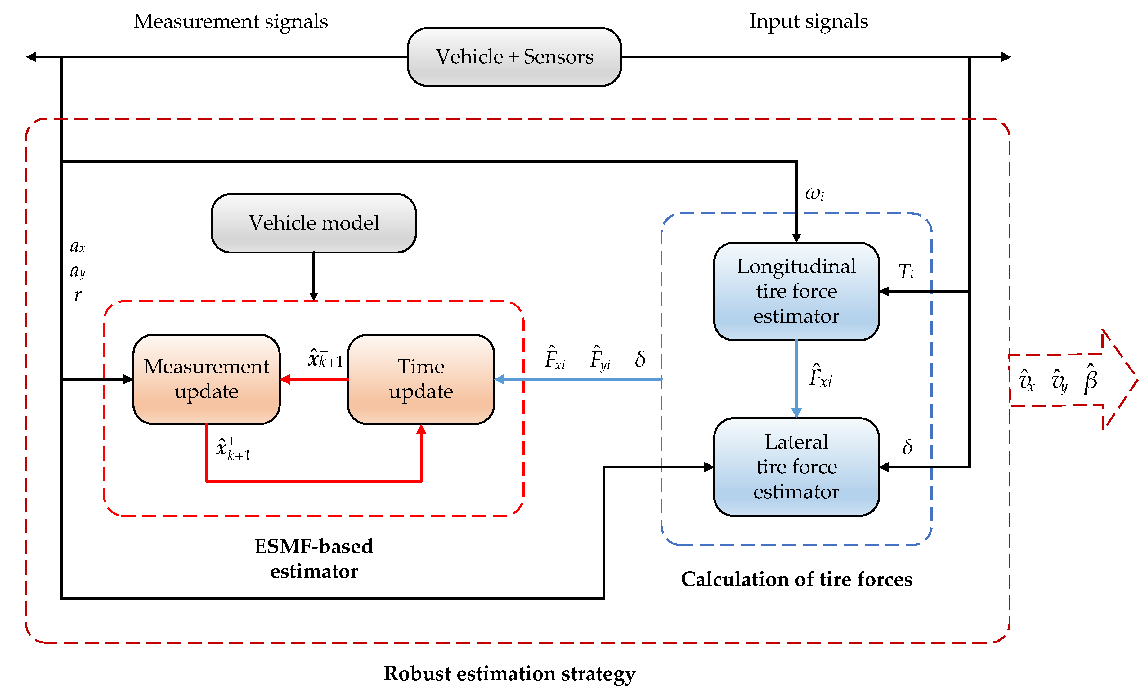
In this study, a robust estimation strategy for vehicle motion states is proposed, which consists of an ESMF-based estimator for vehicle motion states and a KF-based scheme for tire force calculation. The remaining parts of this paper are organized as follows. A dual-track vehicle dynamic model and the design of the robust estimation strategy are discussed in detail in Section 2. The steps of the ESMF algorithm are presented in Section 3. To replace the complex semi-empirical tire models commonly used, Section 4 introduces the scheme of tire force calculation with simple structure. Then Section 5 is devoted to validating the effectiveness of the proposed robust estimation strategy. The last section is the conclusion of this paper.

2. Robust Estimation Strategy for Vehicle Motion States

2.1. Vehicle Model

As the comprehensive consideration of accuracy and simplicity, a commonly used dual-track vehicle dynamic model is established in Figure 1 involving vehicle’s longitudinal, lateral, and yaw motions, where the influence of suspension and vehicle roll motion is ignored.

The dual-track vehicle can be modeled as:

$$\begin{array}{cc}\hfill \dot{r}& =\frac{M_z}{I_z}\hfill \\ \hfill {\dot{v}}_x& =a_x+v_{y}r\hfill \\ \hfill {\dot{v}}_y& =a_y-v_{x}r\hfill \end{array}$$

(1)

where r is the vehicle’s yaw rate, $v_x$ and $v_y$ are the longitudinal and lateral velocities in vehicle’s mass center, $I_z$ is the vehicle’s moment of inertia. The vehile’s yaw moment $M_z$, the longitudinal acceleration $a_x$ and lateral acceleration $a_y$ in vehicle’s mass center in Equation (1) are expressed as:

$$\begin{array}{cc}\hfill a_x& =\frac{(F_{x1}+F_{x2})cos\delta -(F_{y1}+F_{y2})sin\delta +F_{x3}+F_{x4}}{m}\hfill \\ \hfill a_y& =\frac{(F_{x1}+F_{x2})sin\delta +(F_{y1}+F_{y2})cos\delta +F_{y3}+F_{y4}}{m}\hfill \\ \hfill M_z& =a·((F_{x1}+F_{x2})sin\delta +(F_{y1}+F_{y2})cos\delta )-b·(F_{y3}+F_{y4})\hfill \\ \hfill & \phantom{=}-{\displaystyle \frac{t_f}{2}}.((F_{x1}-F_{x2})cos\delta -(F_{y1}-F_{y2})sin\delta )-{\displaystyle \frac{t_r}{2}}·(F_{x3}-F_{x4})\hfill \end{array}$$

(2)

where $\delta$ is the steering angle of front tire, m is the total weight of vehicle, a and b are the distances from vehicle’s mass center to front axle and rear axle, $t_f$ and $t_r$ are the wheelbases of front tires and rear tires, $F_{x1}$, $F_{x2}$, $F_{x3}$ and $F_{x4}$ represent the longitudinal forces of left front tire, right front tire, left rear tire and right rear tire, and $F_{y1}$, $F_{y2}$, $F_{y3}$ and $F_{y4}$ represent the lateral forces of left front tire, right front tire, left rear tire and right rear tire, respectively.

2.2. Design of Robust Estimation Strategy

The proposed strategy is achieved based on the combination of the established vehicle dynamics and estimation algorithms. We choose the robust ESMF algorithm based on the minimal-trace ellipsoid method, which makes it adaptively select the most reasonable parameters to optimize the estimation sets. In addition, considering the problem of numerical stability, the process of interval analysis for bounding truncation error is replaced by appropriately increasing the boundary values of process and measurement noises.

On the basis of Equation (1), the state space of the nonlinear vehicle state estimation can be expressed as:

$$\begin{array}{cc}\hfill \dot{\mathit{x}}& =m(\mathit{x},\mathit{u})+\mathit{w}\hfill \\ \hfill \mathit{z}& =n\left(\mathit{x}\right)+\mathit{v}\hfill \end{array}$$

(3)

where $m\left(\right)$ and $n\left(\right)$ are the process and measurement functions, $\mathit{x}$ is the state vector composed of the longitudinal velocity, lateral velocity, yaw rate, longitudinal acceleration, lateral acceleration and yaw moment, i.e., $\mathit{x}={\left[v_x{v}_{y}r{a}_x{a}_y{M}_z\right]}^{\mathrm{T}}$, $\mathit{z}$ is the measurement vector consisting of the yaw rate, longitudinal acceleration and lateral acceleration, that is, $\mathit{z}={\left[r{a}_x{a}_y\right]}^{\mathrm{T}}$, and $\mathit{w}$ and $\mathit{v}$ are the process and measurement noises, respectively, $\mathit{u}$ is the input of the state estimation system composed by the steering wheel angle and the longitudinal and lateral force of each tire.

The signals in the measurement vector can be directly obtained through the standard sensors equipped on vehicle. The components of the state vector are the vehicle states that need to be estimated, where $a_x$, $a_y$ and r are extended as estimated states to make full use of the measurement information.

To implement a linear/nonlinear estimation algorithm, the continuous system expressed in Equation (3) must be discretized according to the sampling time $▵T$, and the discrete system can be noted as:

$$\begin{array}{c}{\left[\begin{array}{c}{v}_x\\ v_y\\ r\\ a_x\\ a_y\\ M_z\end{array}\right]}_{k+1}={\left[\begin{array}{c}{v}_{y}r+a_x\\ -v_{x}r+a_y\\ \frac{M_z}{I_z}\\ 0\\ 0\\ 0\end{array}\right]}_k·\Delta T+{\left[\begin{array}{c}{v}_x\\ v_y\\ r\\ a_x\\ a_y\\ M_z\end{array}\right]}_k+{\mathit{w}}_k\end{array}$$

(4a)

$$\begin{array}{c}{\mathit{z}}_{k+1}=\left[\begin{array}{cccccc}0& 0& 1& 0& 0& 0\\ 0& 0& 0& 1& 0& 0\\ 0& 0& 0& 0& 1& 0\end{array}\right]·{\mathit{x}}_{k+1}+{\mathit{v}}_{k+1}\end{array}$$

(4b)

where the subscripts k and $k+1$ denote the $k\mathrm{th}$ and $(k+1)\mathrm{th}$ sampling instants.

Apply the steps of the ESMF algorithm in Section 3 to the state space Equation (4), and substitute the result of the tire force calculation in Section 4 into Equation (4). Subsequently, the robust estimation strategy for vehicle motion states can be constructed, which can be found in Figure 2.

The vehicle sideslip angle $\beta$ is approximately calculated through the estimated longitudinal velocity and lateral velocity:

$$\widehat{\beta }\approx arctan\left(\frac{{\widehat{v}}_y}{{\widehat{v}}_x}\right)$$

(5)

3. Extended Set-Membership Filter

The ESMF is an algorithm that relies on unknown but bounded noise. This assumption for noise distribution can be generally satisfied in practical application, which makes the ESMF insensitive to the changes of model and measurement errors. Therefore, it can solve the defect that traditional filtering algorithms obtain the best estimation only with prior knowledge of system noise. The result of the set-membership estimation is a set of feasible solutions, and it can be guaranteed to include the real states. Generally, the center of the ellipsoid set is selected as the estimated value of each time step to make comparison with the real value.

Consider the following discrete form of the state space expressed in Equation (3):

$$\begin{array}{cc}\hfill {\mathit{x}}_{k+1}& =f\left({\mathit{x}}_k\right)+{\mathit{w}}_k\hfill \\ \hfill {\mathit{z}}_{k+1}& =h\left({\mathit{x}}_{k+1}\right)+{\mathit{v}}_{k+1}\hfill \end{array}$$

(6)

where $f\left(\right)$ and $h\left(\right)$ are the process and measurement functions of the discrete system, ${\mathit{x}}_k$ is the $k\mathrm{th}$ system state vector, ${\mathit{z}}_{k+1}$ is the $(k+1)\mathrm{th}$ system measurement vector, ${\mathit{w}}_k$ and ${\mathit{v}}_{k+1}$ are the $k\mathrm{th}$ system process and $(k+1)\mathrm{th}$ measurement noises, respectively, which are assumed to be limited by the following ellipsoid sets:

$$\begin{array}{cc}\hfill {\mathit{W}}_k& =\{{\mathit{w}}_k:{\mathit{w}}_k^{\mathrm{T}}{\mathit{Q}}_k^{-1}{\mathit{w}}_k\le 1\}\hfill \\ \hfill {\mathit{V}}_{k+1}& =\{{\mathit{v}}_{k+1}:{\mathit{v}}_{k+1}^{\mathrm{T}}{\mathit{R}}_{k+1}^{-1}{\mathit{v}}_{k+1}\le 1\}\hfill \end{array}$$

(7)

where $\mathit{Q}={\mathit{Q}}^{\mathrm{T}}$ and $\mathit{R}={\mathit{R}}^{\mathrm{T}}$ are the known and positive definite matrices representing the shape of the ellipsoid sets of the process and measurement noises. Furthermore, the initial state ${\mathit{x}}_0$ belongs to the following ellipsoid set:

$${({\mathit{x}}_0-{\widehat{\mathit{x}}}_0)}^{\mathrm{T}}{\mathit{P}}_0^{-1}({\mathit{x}}_0-{\widehat{\mathit{x}}}_0)\le 1$$

(8)

where ${\widehat{\mathit{x}}}_0$ is the ellipsoid center assumed to be known, ${\mathit{P}}_0={\mathit{P}}_0^{\mathrm{T}}$ is the known and positive definite matrix which denotes the shape of the initial ellipsoid set.

In the ESMF algorithm, the result of the time update, called one-step prediction ${\mathit{E}}_{k+1}^{-}$, is an ellipsoid set containing the vector sum of the state transition set and process noise set:

$${\mathit{E}}_{k+1}^{-}=\{{\mathit{x}}_{k+1}^{-}:{({\mathit{x}}_{k+1}^{-}-{\widehat{\mathit{x}}}_{k+1}^{-})}^{\mathrm{T}}{\left({\mathit{P}}_{k+1}^{-}\right)}^{-1}({\mathit{x}}_{k+1}^{-}-{\widehat{\mathit{x}}}_{k+1}^{-})\le 1\}$$

(9)

where ${\mathit{x}}_{k+1}^{-}$ is the ellipsoid center, ${\mathit{P}}_{k+1}^{-}$ is the matrix that defines its shape, and it should be noted that ${\mathit{E}}_{k+1}^{-}$ is the prior estimated ellipsoid set obtained before the utilization of the measurement vector ${\mathit{z}}_{k+1}$.

The result of the measurement update is an ellipsoid set which contains the intersection of the one-step prediction set and measurement set:

$${\mathit{E}}_{k+1}^{+}=\{{\mathit{x}}_{k+1}^{+}:{({\mathit{x}}_{k+1}^{+}-{\widehat{\mathit{x}}}_{k+1}^{+})}^{\mathrm{T}}{\left({\mathit{P}}_{k+1}^{+}\right)}^{-1}({\mathit{x}}_{k+1}^{+}-{\widehat{\mathit{x}}}_{k+1}^{+})\le 1\}$$

(10)

where ${\mathit{x}}_{k+1}^{+}$ and ${\mathit{P}}_{k+1}^{+}$ are the posterior estimations obtained after utilizing the measurement ${\mathit{z}}_{k+1}$.

On the assumption that $\mathit{F}$ and $\mathit{H}$ are the Jacobian matrices of the discrete system, the specific steps for the ESMF algorithm are as follows:

Time update:

(1)

Determine the center of the one-step prediction ellipsoid set:

$${\widehat{\mathit{x}}}_{k+1}^{-}=f\left({\widehat{\mathit{x}}}_k^{+}\right)$$

(11)

(2)

Update the matrix that defines the shape of the one-step prediction ellipsoid set:

$${\mathit{P}}_{k+1}^{-}=\left(1+\frac{1}{{\gamma }_{k+1}}\right){\mathit{F}}_k{\mathit{P}}_k^{+}{\mathit{F}}_k^{\mathrm{T}}+(1+{\gamma }_{k+1})\mathit{Q}$$

(12)

Measurement update:

(1)

Calculate the filtering gain:

$${\mathit{K}}_{k+1}={\mathit{P}}_{k+1}^{-}{\mathit{H}}_{k+1}^{\mathrm{T}}{\left({\mathit{H}}_{k+1}{\mathit{P}}_{k+1}^{-}{\mathit{H}}_{k+1}^{\mathrm{T}}+\frac{\mathit{R}}{{\lambda }_{k+1}}\right)}^{-1}$$

(13)

(2)

Update the center of the state ellipsoid set:

$$\begin{array}{cc}\hfill {\mathit{e}}_{k+1}& ={\mathit{z}}_{k+1}-h\left({\widehat{\mathit{x}}}_{k+1}^{-}\right)\hfill \end{array}$$

(14)

$$\begin{array}{cc}\hfill {\widehat{\mathit{x}}}_{k+1}^{+}& ={\widehat{\mathit{x}}}_{k+1}^{-}+{\mathit{K}}_{k+1}{\mathit{e}}_{k+1}\hfill \end{array}$$

(15)

(3)

Update the matrix that defines the shape of the ellipsoid set:

$$\begin{array}{cc}\hfill {\mathit{P}}_{k+1}^{+}& ={\rho }_{k+1}\left((\mathit{I}-{\mathit{K}}_{k+1}{\mathit{H}}_{k+1}){\mathit{P}}_{k+1}^{-}{(\mathit{I}-{\mathit{K}}_{k+1}{\mathit{H}}_{k+1})}^{\mathrm{T}}+\frac{1}{{\lambda }_{k+1}}{\mathit{K}}_{k+1}\mathit{R}{\mathit{K}}_{k+1}^{\mathrm{T}}\right)\hfill \end{array}$$

(16)

$$\begin{array}{cc}\hfill {\rho }_{k+1}& =1+{\lambda }_{k+1}-{\mathit{e}}_{k+1}^{\mathrm{T}}{\left(\frac{\mathit{R}}{{\lambda }_{k+1}}+{\mathit{H}}_{k+1}{\mathit{P}}_{k+1}^{-}{\mathit{H}}_{k+1}^{\mathrm{T}}\right)}^{-1}{\mathit{e}}_{k+1}\hfill \end{array}$$

(17)

In Equations (12) and (17), $\gamma$ and $\lambda$ are the variable parameters, and their values directly determine the matrix $\mathit{P}$ representing the size of the ellipsoid. For the time update and measurement update, there are countless choices of ellipsoid sets. Therefore, the choice for the parameters $\gamma$ and $\lambda$ can be viewed as a self-adapting way of the algorithm. In this case, we choose the set that minimizes the trace of the matrix $\mathit{P}$, that is, the minimal-trace ellipsoid method. At this point, the expressions of $\gamma$ and $\lambda$ are as follows:

$$\begin{array}{c}{\gamma }_{k+1}=\sqrt{\frac{\mathrm{tr}\left({\mathit{F}}_k{\mathit{P}}_k^{+}{\mathit{F}}_k^{\mathrm{T}}\right)}{\mathrm{tr}\left(\mathit{Q}\right)}},{\gamma }_{k+1}>0\end{array}$$

(18)

$$\begin{array}{c}{\lambda }_{k+1}=\arg \min \left({\rho }_{k+1}\mathrm{tr}\left((\mathbf{I}-{\mathit{K}}_{k+1}{\mathit{H}}_{k+1}){\mathit{P}}_{k+1}^{-}\right)\right),{\lambda }_{k+1}\ge 0\end{array}$$

(19)

4. Calculation of Tire Forces

At present, the Magic Formula [6,10,12,14,23], HSRI tire model [7,24], Dugoff tire model [5,15] and some other ones have been widely used for the practical application of acquiring vehicle information. When the road adhesion coefficient in the mathematical model is assumed as constant, remarkable model errors occur subsequently. Therefore, an online estimator needs to be adopted to identify road conditions for the use of these semi-empirical models. On the other hand, system model inevitably remains strong nonlinearity even though some considerable simplifications are made. These make it difficult for the design of the online estimator [25,26]. To address this issue, observer theory is introduced by some researchers. The observer-based method is a good choice for indirectly obtaining the tire forces through vehicle dynamics, where the construction of a semi-empirical tire model is replaced, such as the sliding-mode observers (SMO) designed in [27], and the PID-based observer and adaptive-sliding-mode observer (ASMO) designed in [28]. However, for the observer-based method, the effect of system noise is not taken into account.

To a certain extent, filtering algorithm can deal with it by establishing the state and measurement equations with the process and measurement noises. From the perspective of design complexity, in this study, a KF-based scheme is proposed to construct the longitudinal and lateral tire force estimators. This scheme takes the tire forces as a part of the states to be estimated without any prior knowledge of the tire-road friction model. The longitudinal force estimator is built by use of a tire rolling dynamic model, and the lateral force estimator is realized by means of a single-track vehicle dynamic model. The advantage of this scheme is that it can not only alleviate the computation burden, but also enhance the robustness of state estimation due to its insensitivity to the change of road conditions.

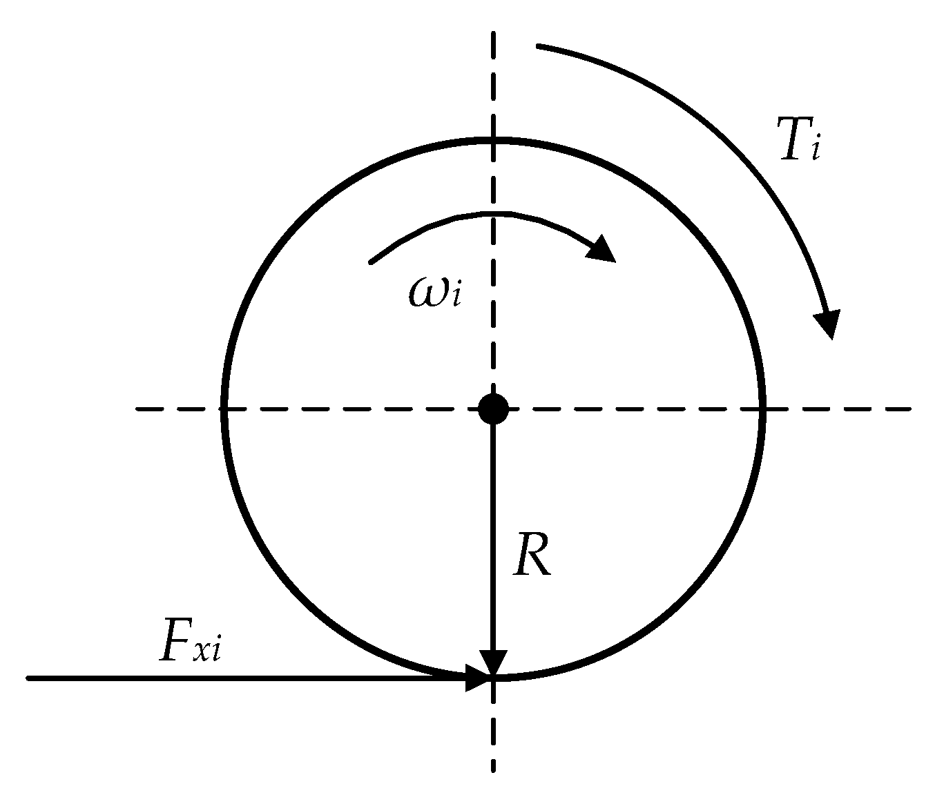
4.1. Longitudinal Tire Force Estimator

As shown in Figure 3, the single tire is modeled as a rigid body that rotates around its mass center.

Ignoring the influence of rolling resistance, the rolling dynamics satisfies:

$$I_w{\dot{\omega }}_i=T_i-F_{xi}R$$

(20)

where $I_w$ and R are the rolling inertia and radius, respectively, ${\omega }_i(i=1,2,3,4)$ represents the tire revolving speed of each tire, and $T_i(i=1,2,3,4)$ is the tire torque of each tire, namely, the sum of the braking and driving torques.

The state space for the longitudinal force estimator is expressed as:

$$\begin{array}{cc}\hfill {\dot{\mathit{x}}}_a& ={\mathit{F}}_a{\mathit{x}}_a+{\mathit{G}}_a{\mathit{u}}_a+{\mathit{w}}_a\hfill \\ \hfill {\mathit{z}}_a& ={\mathit{H}}_a{\mathit{x}}_a+{\mathit{v}}_a\hfill \end{array}$$

(21)

The state vector, input vector and measurement vector are chosen as follows:

State vector: ${\mathit{x}}_a={\left[F_{xi}{\omega }_i\right]}^{\mathrm{T}}$;

Input vector: ${\mathit{u}}_a={\left[T_i\right]}^{\mathrm{T}}$;

Measurement vector: ${\mathit{z}}_a={\left[{\omega }_i\right]}^{\mathrm{T}}$.

Consequently, according to Equation (20), the state transition matrix ${\mathit{F}}_a$, input transition matrix ${\mathit{G}}_a$ and measurement matrix ${\mathit{H}}_a$ in the state equation and measurement equation are as follows:

$${\mathit{F}}_a=\left[\begin{array}{cc}\multicolumn{2}{c}{{\mathit{0}}_{4\times 8}}\\ -{\displaystyle \frac{R}{I_w}}·{\mathit{I}}_{4\times 4}& {\mathit{0}}_{4\times 4}\end{array}\right],{\mathit{G}}_a=\left[\begin{array}{c}{\mathit{0}}_{4\times 4}\\ {\displaystyle \frac{1}{I_w}}·{\mathit{I}}_{4\times 4}\end{array}\right],{\mathit{H}}_a=\left[\begin{array}{cc}{\mathit{0}}_{4\times 4}& {\mathit{I}}_{4\times 4}\end{array}\right]$$

The estimated results are obtained through the iteration of the time update process and the measurement update process in the KF algorithm.

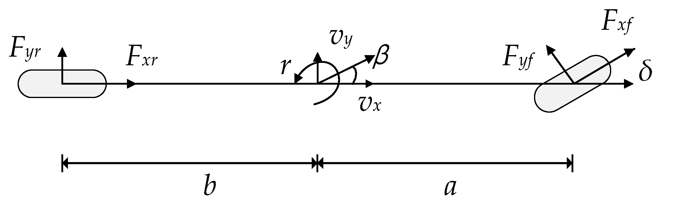
4.2. Lateral Tire Force Estimator

In order to facilitate the construction of lateral force estimator, some simplifications are made on the dual-track vehicle dynamics model mentioned in Section 2.1. This is conducive to simplifying the calculation formulas for state variables [28] with minor effect on the overall idea of vehicle dynamic behavior. Figure 4 shows the established single-track model.

According to Newton’s second law and rotational equilibrium, the vehicle’s lateral motion and vertical rotation can be expressed by the following equations:

$$\left\{\begin{array}{c}m{a}_y=F_{yf}cos\delta +F_{xf}sin\delta +F_{yr}\hfill \\ I_z\dot{r}=a{F}_{yf}cos\delta +a{F}_{xf}sin\delta -b{F}_{yr}\hfill \end{array}\right.$$

(22)

where $F_{xf}$ and $F_{xr}$ represent the longitudinal resultant forces of two front tires and two rear tires, and $F_{yf}$ and $F_{yr}$ represent their lateral resultant forces, respectively.

Based on Equation (22), the lateral forces $F_{yf}$ and $F_{yr}$ are rewritten as follows:

$$\left\{\begin{array}{c}{F}_{yf}={\displaystyle \frac{bm{a}_y+I_z\dot{r}-F_{xf}(a+b)sin\delta }{(a+b)cos\delta }}\hfill \\ F_{yr}={\displaystyle \frac{am{a}_y-I_z\dot{r}}{a+b}}\hfill \end{array}\right.$$

(23)

With the purpose of enhancing the estimation accuracy, lateral forces $F_{yf}$ and $F_{yr}$ computed from Equation (23) are treated as one part of the measurement values, where they are denoted as $F_{yf}^{\mathrm{com}}$ and $F_{yr}^{\mathrm{com}}$. It is feasible because their values can be acquired by utilizing onboard sensors signals, namely, the steering wheel angle, yaw rate and lateral acceleration. As a result, the state vector and measurement vector for the lateral tire force estimator are chosen as follows.

State vector: ${\mathit{x}}_b={\left[F_{yf}{F}_{yr}r\right]}^{\mathrm{T}}$;

Measurement vector: ${\mathit{z}}_b={\left[F_{yf}^{\mathrm{com}}{F}_{yr}^{\mathrm{com}}r{a}_y\right]}^{\mathrm{T}}$.

The state space for lateral force estimator is expressed as:

$$\begin{array}{cc}\hfill {\dot{\mathit{x}}}_b& ={\mathit{F}}_b{\mathit{x}}_b+{\mathit{u}}_{b1}+{\mathit{w}}_{\mathit{b}}\hfill \\ \hfill {\mathit{z}}_b& ={\mathit{H}}_b{\mathit{x}}_b+{\mathit{u}}_{b2}+{\mathit{v}}_b\hfill \end{array}$$

(24)

The corresponding state transition matrix ${\mathit{F}}_b$, measurement matrix ${\mathit{H}}_b$ and input vectors ${\mathit{u}}_{b1}$, ${\mathit{u}}_{b2}$ are as follows:

$$\begin{array}{c}{\mathit{F}}_b=\left[\begin{array}{ccc}\multicolumn{3}{c}{{\mathit{0}}_{2\times 3}}\\ {\displaystyle \frac{cos\delta ·a}{I_z}}& -{\displaystyle \frac{b}{I_z}}& 0\end{array}\right],{\mathit{H}}_b=\left[\begin{array}{ccc}\multicolumn{3}{c}{{\mathit{I}}_{3\times 3}}\\ {\displaystyle \frac{cos\delta }{m}}& {\displaystyle \frac{1}{m}}& 0\end{array}\right],\\ {\mathit{u}}_{b1}={\left[\begin{array}{ccc}0& 0& {\displaystyle \frac{a}{I_z}}{F}_{xf}sin\delta \end{array}\right]}^{\mathrm{T}},{\mathit{u}}_{b2}={\left[\begin{array}{cccc}0& 0& 0& {\displaystyle \frac{F_{xf}sin\delta }{m}}\end{array}\right]}^{\mathrm{T}}\end{array}$$

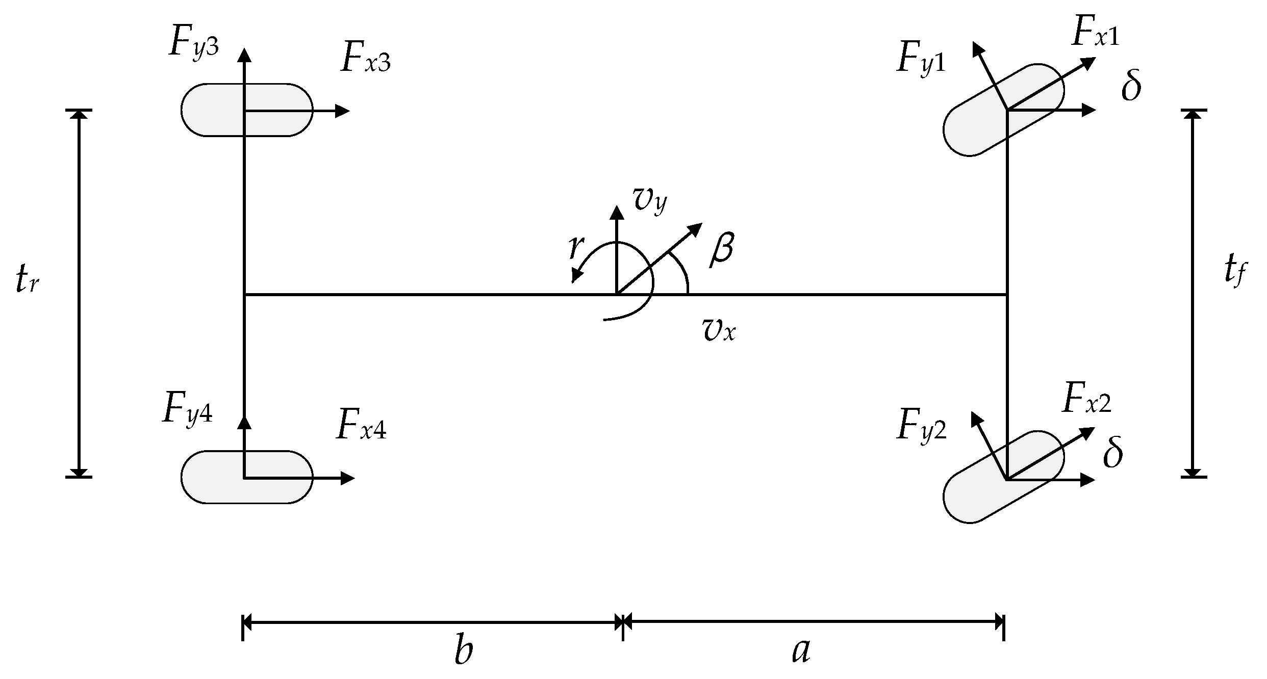
Furthermore, the aspect of the load transfer between left and right tires should also be taken into account because the lateral force of each tire are required in the robust estimation strategy. According to the proportional relationships between the vertical loads of each tire on the same axis, the lateral resultant forces can be decomposed into different components for each tire.

$$\begin{array}{cc}\hfill F_{y1}& =F_{yf}\frac{F_{z1}}{(F_{z1}+F_{z2})}\hfill \\ \hfill F_{y2}& =F_{yf}\frac{F_{z2}}{(F_{z1}+F_{z2})}\hfill \\ \hfill F_{y3}& =F_{yr}\frac{F_{z3}}{(F_{z3}+F_{z4})}\hfill \\ \hfill F_{y4}& =F_{yr}\frac{F_{z4}}{(F_{z3}+F_{z4})}\hfill \end{array}$$

(25)

where the expressions of the loads on each tire $F_{zi}(i=1,2,3,4)$ are shown in Equation (26), which includes the static load, longitudinally transferred load and laterally transferred load.

$$\begin{array}{cc}\hfill F_{z1}& =\frac{mgb}{2(a+b)}-\frac{m{a}_{x}h}{2(a+b)}-\frac{m{a}_{y}hb}{(a+b)t_f}\hfill \\ \hfill F_{z2}& =\frac{mgb}{2(a+b)}-\frac{m{a}_{x}h}{2(a+b)}+\frac{m{a}_{y}hb}{(a+b)t_f}\hfill \\ \hfill F_{z3}& =\frac{mga}{2(a+b)}+\frac{m{a}_{x}h}{2(a+b)}-\frac{m{a}_{y}ha}{(a+b)t_r}\hfill \\ \hfill F_{z4}& =\frac{mga}{2(a+b)}+\frac{m{a}_{x}h}{2(a+b)}+\frac{m{a}_{y}ha}{(a+b)t_r}\hfill \end{array}$$

(26)

4.3. Evaluation of Tire Force Estimator

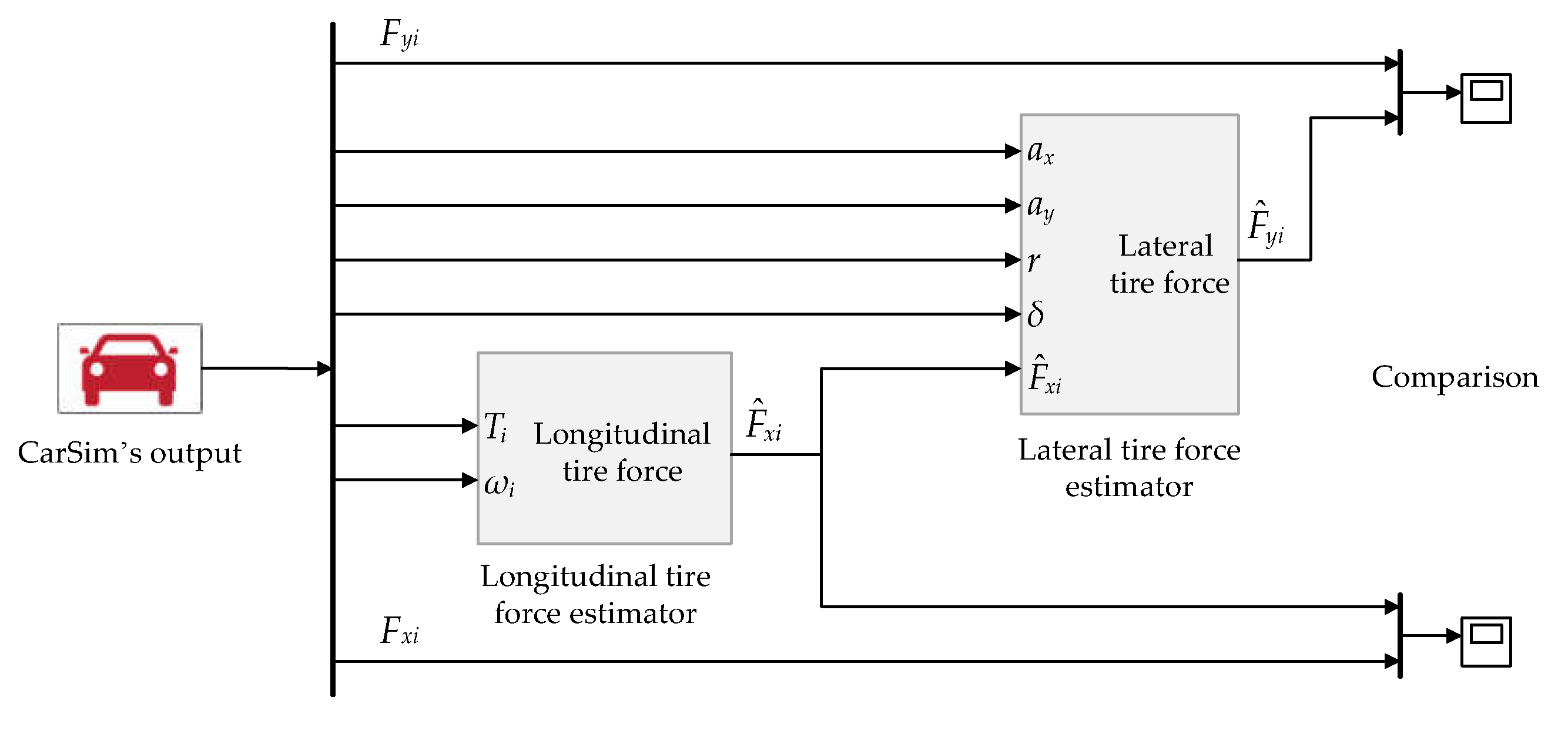
Numerical experiment is implemented via CarSim (a professional software widely used in automotive industry) and Matlab/Simulink co-simulation to testify the performance of the scheme chosen for the estimation of the tire forces.

Figure 5 shows the structure for the calculation of tire forces, where the output signals of CarSim are taken as the inputs of the tire force estimators at each sampling instant. The longitudinal and lateral tire force estimators are built by use of the “S-Function” module in Simulink, where the corresponding algorithm code are integrated.

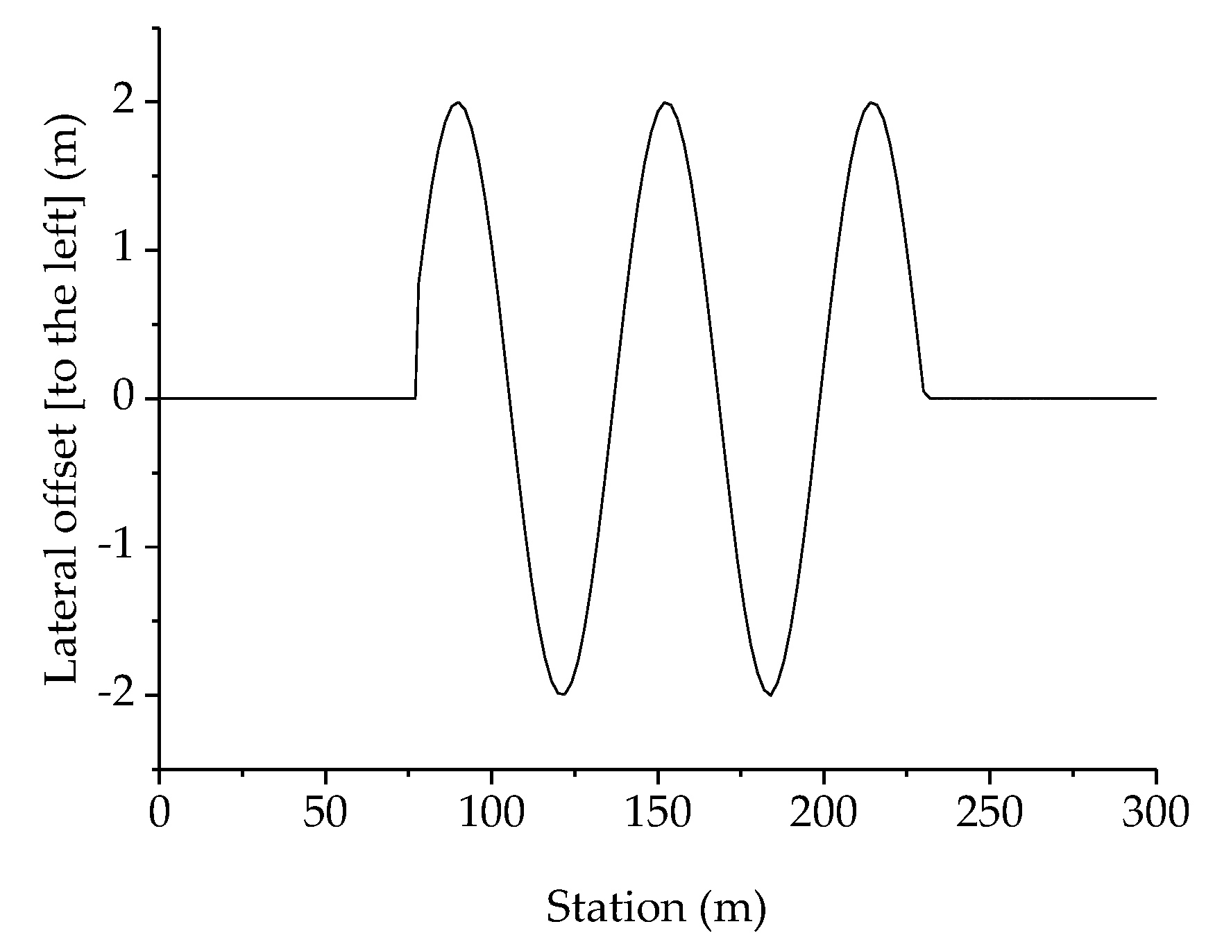
A front-wheel driven vehicle is selected and set to move at a constant speed of $120\mathrm{km}/\mathrm{h}$ along the route depicted in Figure 6. The corresponding results obtained from these two estimators are used to make comparison with the reference values of the tire forces output by CarSim.

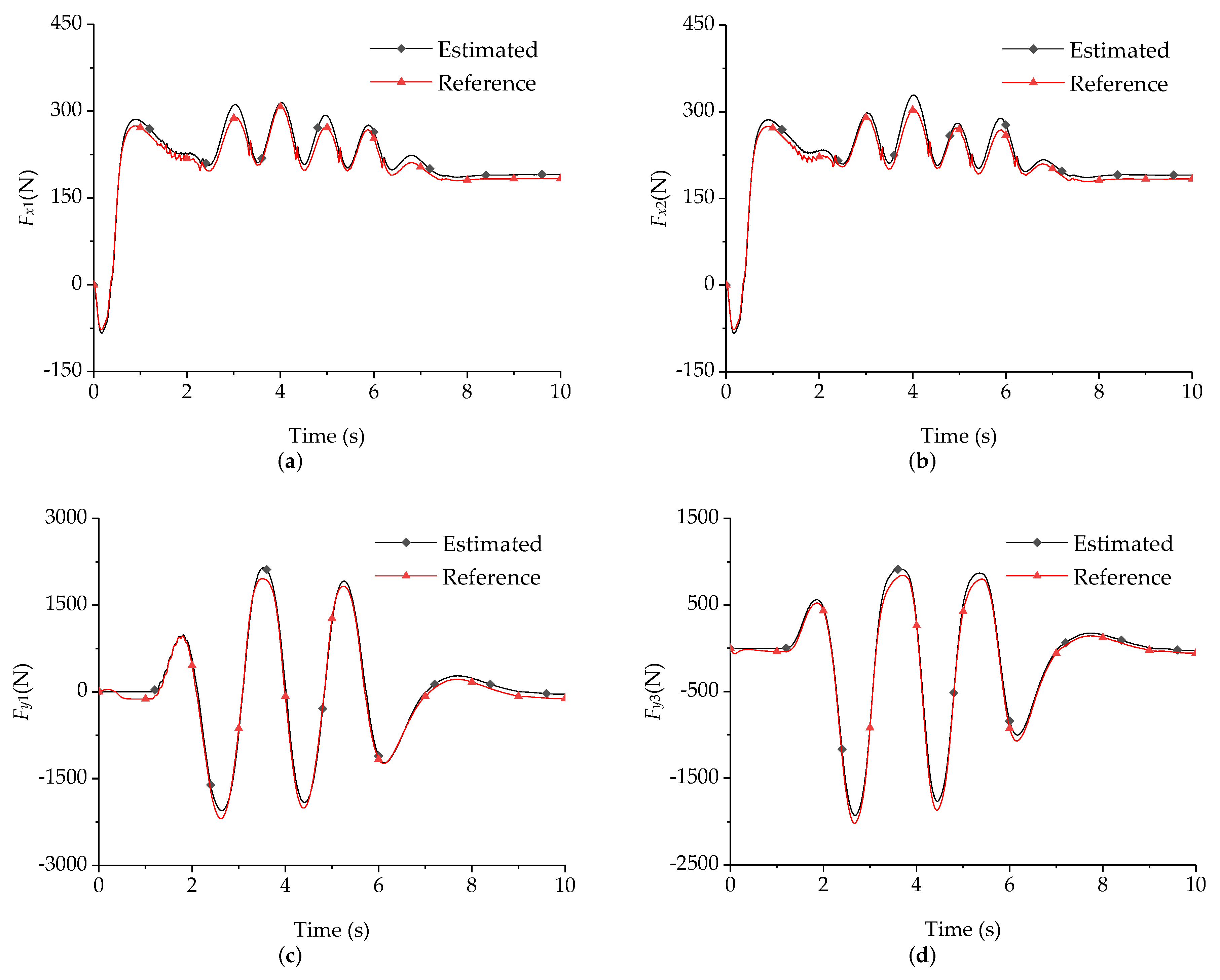
Noticing that the vehicle is driven by front wheels, some representative estimation results are presented in Figure 7 for the convenience of analysis, where the longitudinal forces of two front tires and the lateral forces of two left tires are included.

It can be seen from Figure 7 that the estimated longitudinal forces for left and right front tires match the reference curves well, where the maximum errors of about $7.5\%$ and $8.9\%$ occur at around time points $3\mathrm{s}$ and $4\mathrm{s}$, respectively.

For the estimated lateral force of left front tire in Figure 7c, deviation appears at the first few seconds of vehicle motion. The reason for this is the insufficient lateral excitation from ground. After the steering wheel angle starts working, the estimated results almost match the reference values, except for some moments when the vehicle is just in high maneuvers. For example, around time points $2.6\mathrm{s}$, $3.5\mathrm{s}$, $4.4\mathrm{s}$ and $5.3\mathrm{s}$. The reason for the deviations at these moments can be ascribed to the neglected role of the suspension in vehicle dynamic model.

The performance of the adopted scheme can be further evaluated by the normalized root-mean-square (NRMS) of the corresponding estimated result [28], which is calculated as follows:

$$\mathrm{NRMS}={\displaystyle \frac{\sqrt{\sum _{i=1}^n{\displaystyle \frac{{(F_{\mathrm{reference}}-{\widehat{F}}_{\mathrm{estimated}})}^2}{n}}}}{\max \left(\left|F_{\mathrm{reference}}\right|\right)}}$$

(27)

where $F_{\mathrm{reference}}$ is the reference value of tire force, ${\widehat{F}}_{\mathrm{estimated}}$ is the estimated value, and n is the sampling number. For the estimation results in Figure 7, the NRMSs of $F_{x1}$, $F_{x2}$, $F_{y1}$ and $F_{y3}$ are $3.44\%$, $3.56\%$, $4.10\%$ and $2.76\%$, respectively, which shows that the accuracy of the estimated tire force is acceptable.

Based on the above scheme with simple structure, the calculation of tire forces can be provided with good accuracy, where no knowledge of road adhesion coefficient is needed. Therefore, it is likely to be adopted in some practical applications. In the following part of this paper, the output results of the tire force estimators are taken as one portion of the input of the proposed robust estimation strategy.

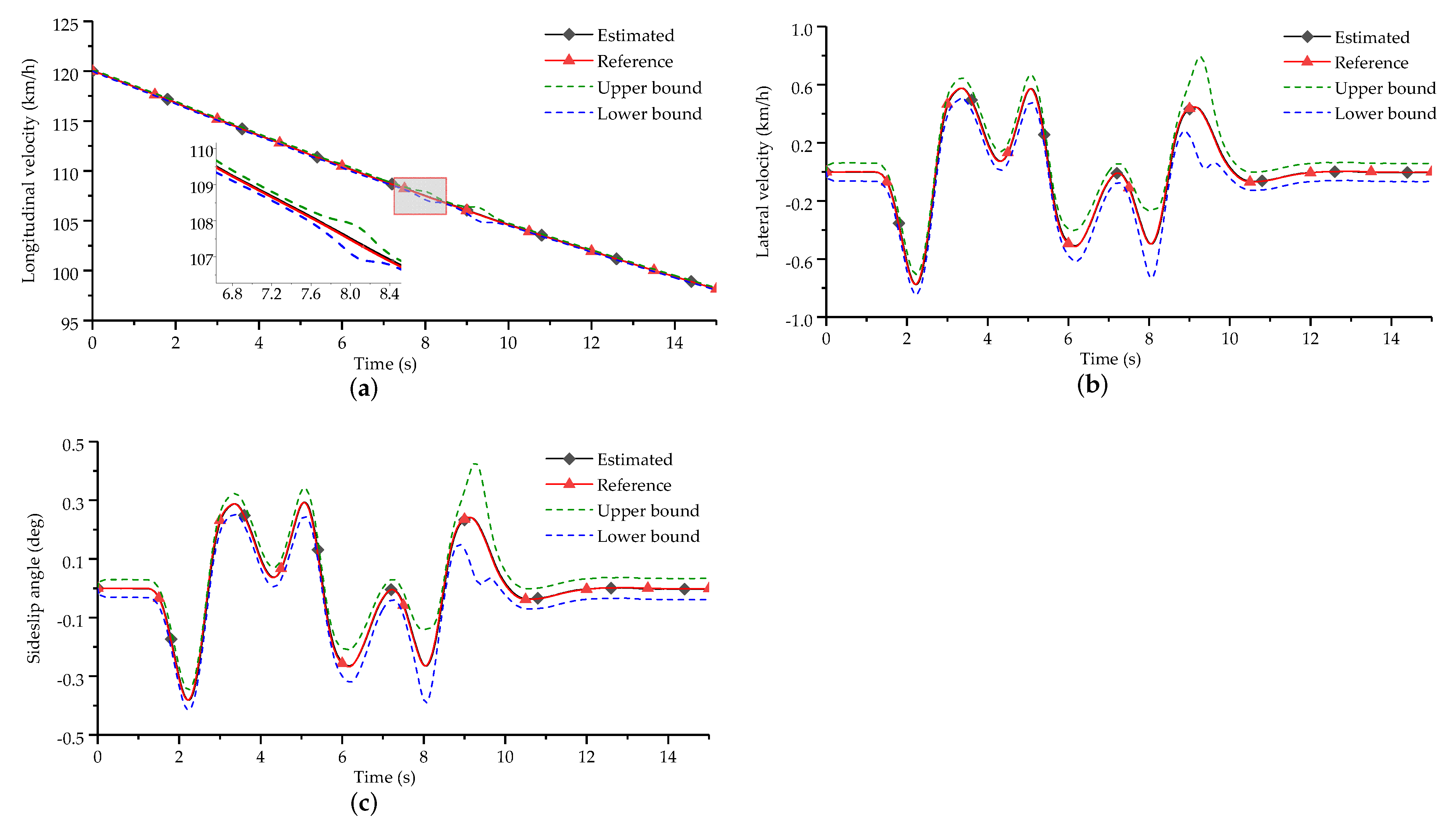
5. Verification for Robust Estimation Strategy

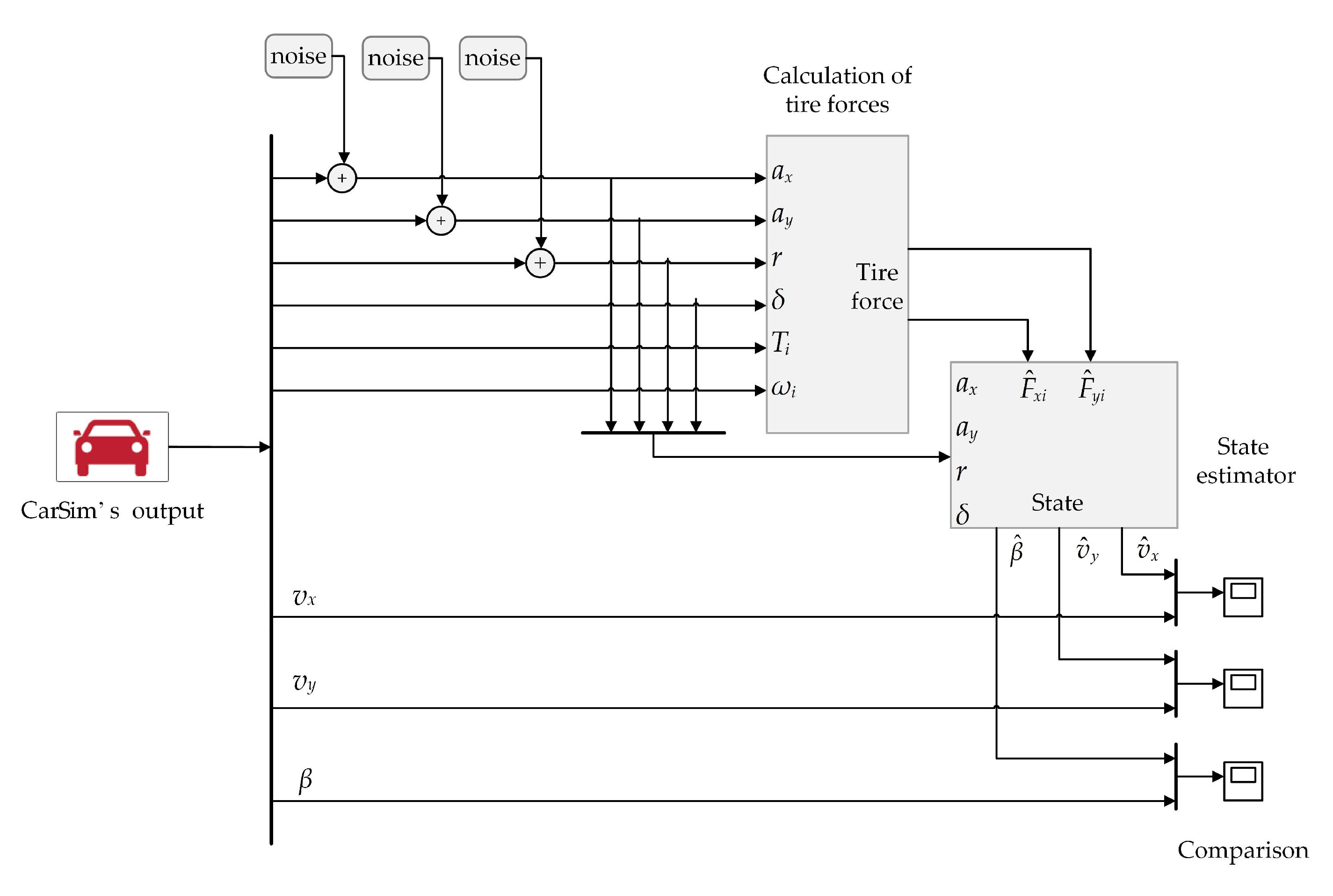
In order to verify the effectiveness of the proposed robust estimation strategy based on the ESMF algorithm, a series of numerical experiments are carried out employing CarSim and Matlab/Simulink.

The verification structure for the proposed robust estimation strategy is shown in Figure 8. The input of the ESMF-based vehicle state estimator is composed of the basic signals output by CarSim and the result obtained from the calculation of tire forces. The algorithm steps for vehicle state estimator are also integrated via the “S-Function” module. Moreover, during the whole simulation, the noises with the bounds of $[-0.003,0.003]$, $[-0.003,0.003]$ and $[-0.0001,0.0001]$ are added on the signals including the longitudinal acceleration, lateral acceleration and yaw rate to simulate the practical measurement signals, respectively. The sampling time is set as $0.01\mathrm{s}$.

Vehicle parameters are set as: $m=1416\mathrm{kg}$, $I_z=1523\mathrm{kg}·{\mathrm{m}}^2$, $a=1.106\mathrm{m}$, $b=1.562\mathrm{m}$, $t_f=t_r=1.539\mathrm{m}$, $R=0.31\mathrm{m}$. The double lane change (DLC) maneuver and slalom maneuver are respectively set in CarSim for verification. Furthermore, considering that the UKF is most widely used in the traditional estimation strategies, we present the estimation results using the UKF-based strategy and the reference values from CarSim for making comparison.

5.1. Experimental Results

5.1.1. DLC Maneuver

The selected vehicle performs the DLC maneuver on flat road at an initial speed of $120\mathrm{km}/\mathrm{h}$. For the ESMF-based strategy, the bounds of the process noise and measurement noise are set as: $\left|w_i\right|\le {10}^{-3}$, $\left|v_1\right|\le 3\times {10}^{-3}$, $|v_2|\le 3\times {10}^{-3}$, $\left|v_3\right|\le {10}^{-4}$. The corresponding ellipsoid shape matrices which define the process and measurement noises are set as:

$$\mathit{Q}={\mathit{I}}_{6\times 6}\times {10}^{-5},\mathit{R}=\left[\begin{array}{ccc}{10}^{-4}& 0& 0\\ 0& {10}^{-4}& 0\\ 0& 0& {10}^{-7}\end{array}\right]$$

The center and matrix that define the shape of the initial state ellipsoid are initialized as follow:

$${\mathit{x}}_0={\left[\begin{array}{cccccc}{\displaystyle \frac{120}{3.6}}& 0& 0& 0& 0& 0\end{array}\right]}^{\mathrm{T}},{\mathit{P}}_0={\mathit{I}}_{6\times 6}\times {10}^{-2}$$

The ellipsoidal projection $\widehat{\mathit{x}}\pm \mathit{E}z$ [29] can be taken as the upper and lower bounds (see the dot lines in Figure 9) of the estimated results, where $\mathit{P}=\mathit{E}{\mathit{E}}^{\mathrm{T}}$, and $\parallel \mathit{z}\parallel \le 1$.

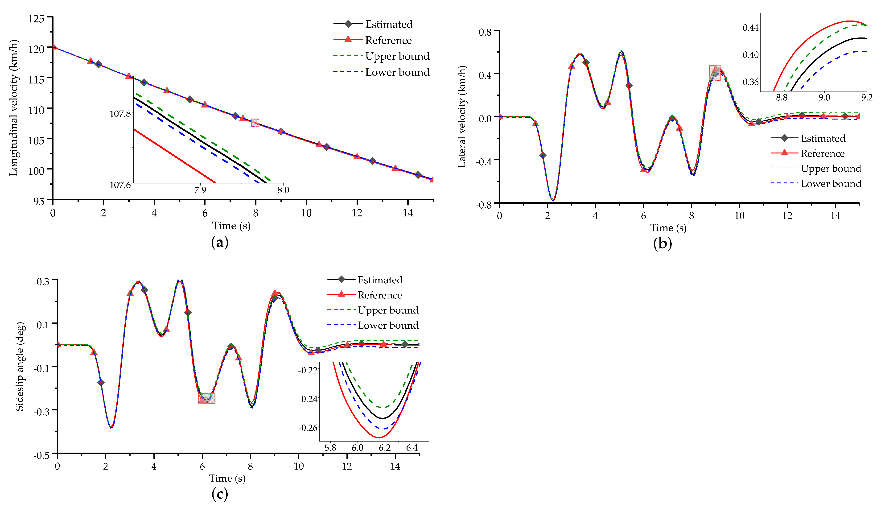
For the UKF-based strategy, the initial value, process noise’s covariance matrix $\mathit{Q}$, measurement noise’s covariance matrix $\mathit{R}$, and initial error covariance matrix ${\mathit{P}}_0$ are set as follows, respectively:

$${\mathit{x}}_0={\left[\begin{array}{cccccc}{\displaystyle \frac{120}{3.6}}& 0& 0& 0& 0& 0\end{array}\right]}^{\mathrm{T}},\mathit{Q}={\mathit{I}}_{6\times 6}\times {10}^{-6},\mathit{R}=\left[\begin{array}{ccc}{10}^{-6}& 0& 0\\ 0& {10}^{-6}& 0\\ 0& 0& {10}^{-9}\end{array}\right],{\mathit{P}}_0={\mathit{I}}_{6\times 6}\times {10}^{-3}$$

Moreover, as the consideration of the mathematical principle for a stochastic distribution, the expression of $\widehat{\mathit{x}}\pm 3\sigma$ is chosen as the upper and lower bounds (see the dot lines in Figure 10) of the estimated results of the UKF-based strategy.

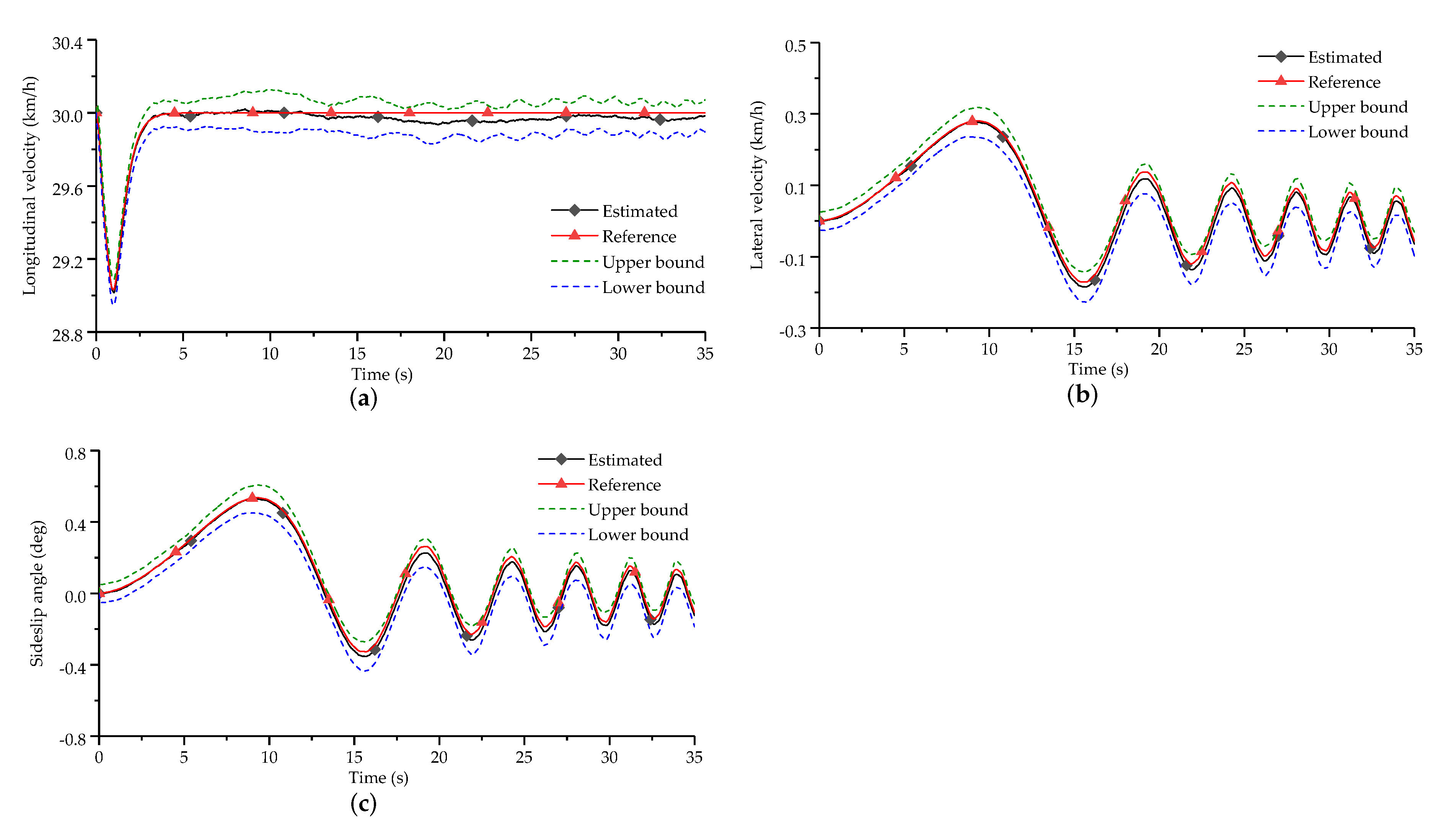
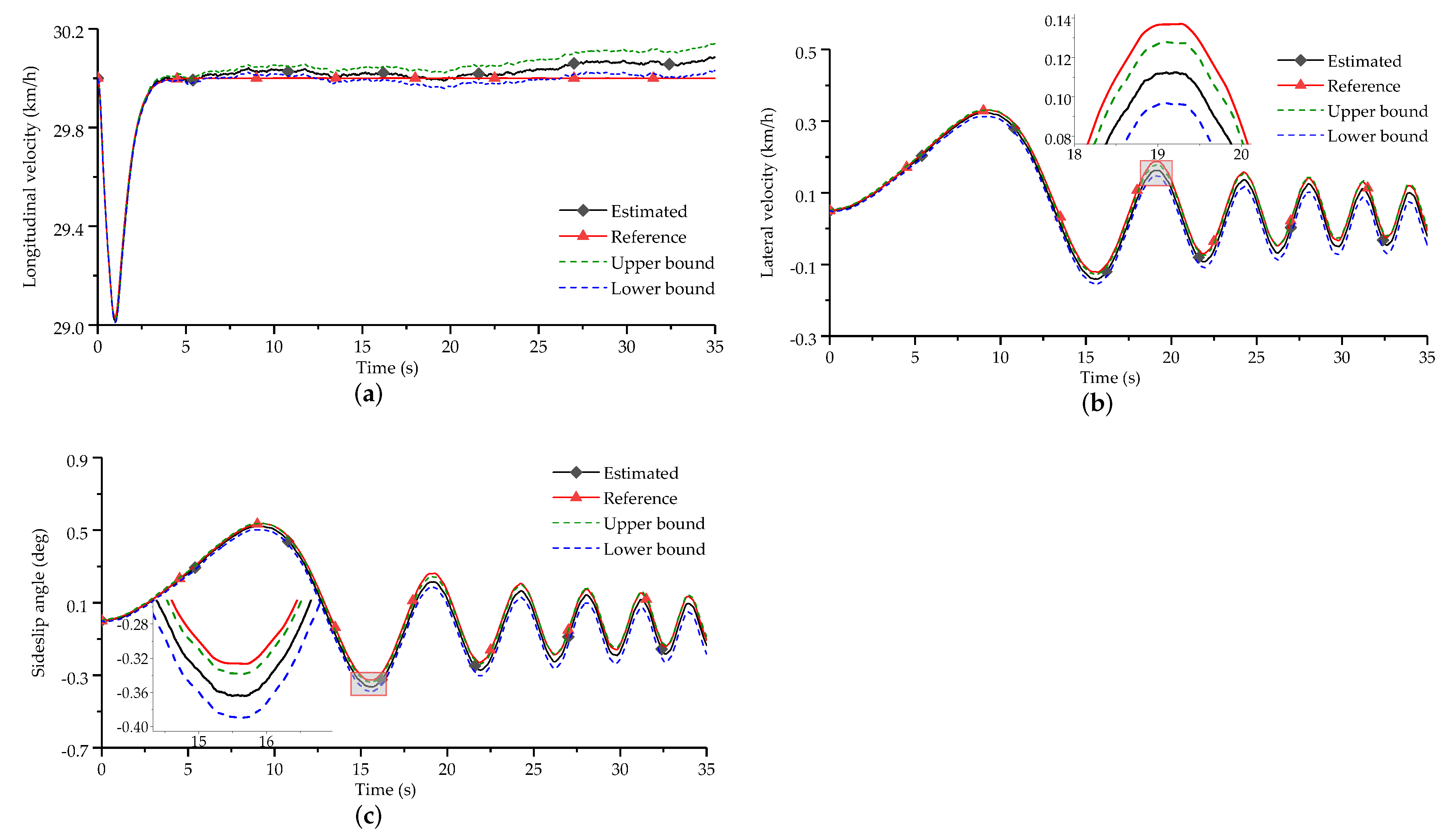
5.1.2. Slalom Maneuver

Under the slalom maneuver, vehicle moves on flat road at an initial speed of $30\mathrm{km}/\mathrm{h}$, where the selection of the other conditions and parameters are same as those in the DLC experiment except for ${\mathit{x}}_0$, i.e., ${\mathit{x}}_0={[30/3.600000]}^{\mathrm{T}}$. The vehicle state estimation results based on the ESMF and UKF algorithms are shown in Figure 11 and Figure 12.

5.2. Result Analysis

It can be found from Figure 9 and Figure 11 that the reference values of the states are contained within the hard bounds consisting of the upper bound and lower bound provided by the proposed ESMF-based strategy. When the value of the lateral velocity reaches its local peak or valley, the boundary range also becomes large. Especially, at around time points 8 s and 9.5 s in Figure 9, this phenomenon is obvious.

As shown in Figure 10 and Figure 12, the hard bounds provided by the UKF do not contain the reference values of the states at some moments, especially at the top or bottom of the estimated curves. As shown by time intervals $[8.7\mathrm{s},9.2\mathrm{s}]$ in Figure 10b and $[5.7\mathrm{s},6.5\mathrm{s}]$ in Figure 10c, the reference values of the lateral velocity and vehicle sideslip angle are out of the range restricted by the upper and lower bounds. Similar situations illustrated by time intervals $[18\mathrm{s},20\mathrm{s}]$ in Figure 12b and $[14\mathrm{s},17\mathrm{s}]$ in Figure 12c also illustrate this phenomenon.

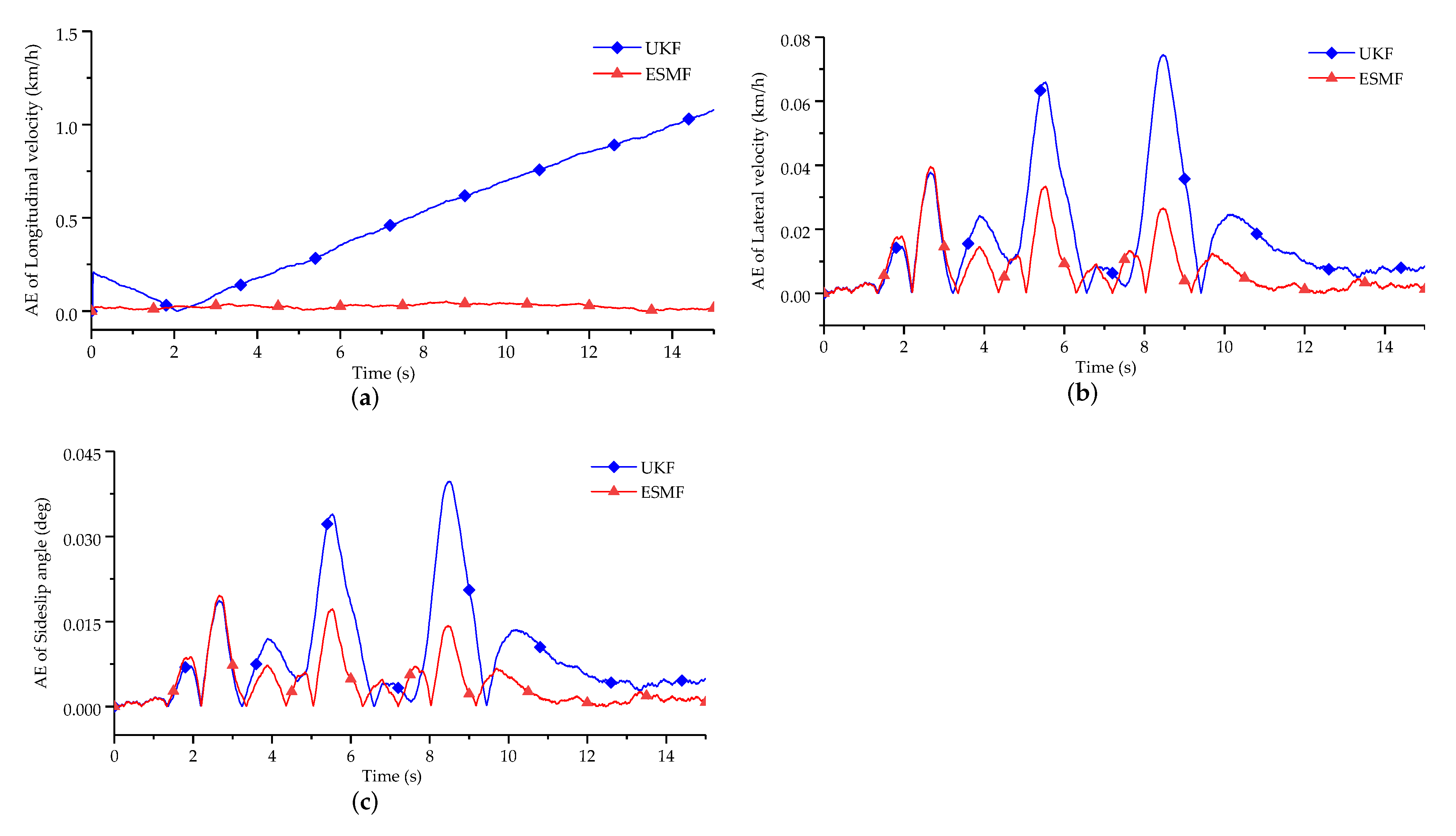
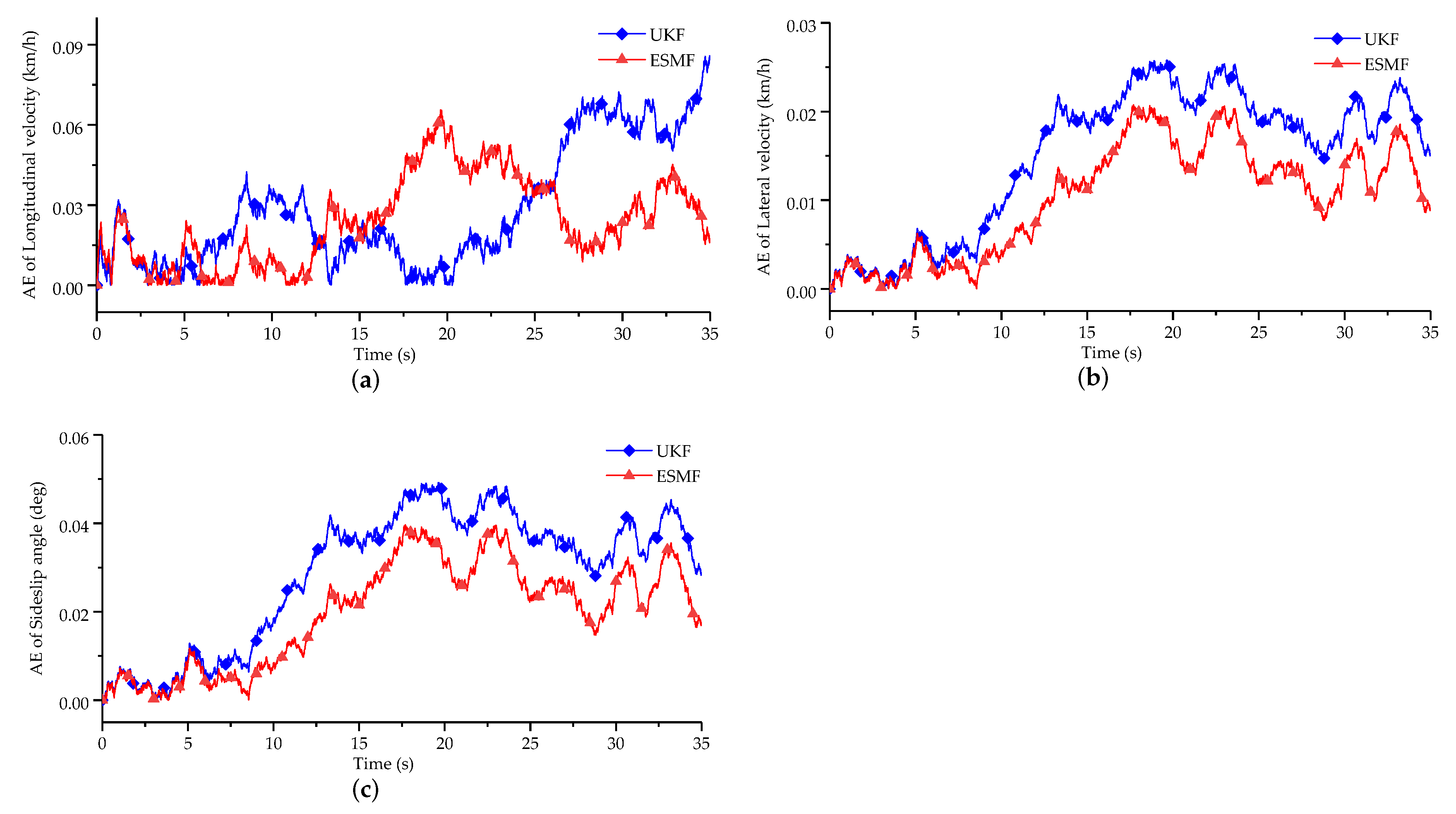
Furthermore, to clearly quantify the performance of superiority, visualized curves and statistical values are utilized, i.e., the absolute error (AE) curves and root mean square errors (RMSEs) between the estimated and reference values of these two strategies. As shown in Figure 13 and Figure 14 and

Table 2. RMSEs under the DLC maneuver.

	${\mathit{v}}_{\mathit{x}}$ (km/h)	${\mathit{v}}_{\mathit{y}}$ (km/h)	$\mathit{\beta }$ (deg)
UKF	0.08663	0.02424	0.01276
ESMF	0.02747	0.01144	0.005864

and

Table 3. RMSEs under the slalom maneuver.

	${\mathit{v}}_{\mathit{x}}$ (km/h)	${\mathit{v}}_{\mathit{y}}$ (km/h)	$\mathit{\beta }$ (deg)
UKF	0.03610	0.01701	0.03248
ESMF	0.02923	0.01203	0.02301

, the AE curves in both two cases based on the ESMF algorithm are under those based on the UKF one in most time, and the RMSEs of the former are also less than the latter.

In brief, utilizing the ESMF-based strategy can not only acquire the estimation results with good accuracy but also provide $100\%$ confidence for the estimated vehicle motion states, which is the vital performance of robustness for vehicle state estimation.

Additionally, the running time of the vehicle state estimation employing these two strategies is listed in

Table 4. Running time.

Maneuver	Running Time (s)
	ESMF-Based	UKF-Based
DLC	0.466	0.816
Slalom	1.017	1.841

, which shows that under the same maneuver, the ESMF-based strategy needs less time to realize the estimation of vehicle states as compared with the UKF-based one. Therefore, no higher hardware configuration will be required in the practical application of the presented strategy.

5.3. Discussion

On the basis of the above analysis for the experimental results, we can see that the proposed estimation strategy is superior to the UKF-based one on the performance of no matter accuracy or running time. Besides that, hard bounds containing the real vehicle states are always guaranteed when the ESMF-based strategy is implemented. Therefore, good robustness can be acquired for the dynamic deviation from the reference value. However, the UKF-based estimation strategy cannot achieve this, especially when the vehicle’s high maneuver occurs.

The reason for these phenomena is that the ESMF algorithm inherently treats the distribution of the process and measurement noises as unknown but bounded. When the system uncertainty is included in the bounded noise range defined by algorithm requirement, the ESMF-based strategy performs good ability of robustness. Because it is not sensitive to the process noise representing system modelling errors and the noises existing in measurement signals. However, for the commonly used filtering methods, such as the UKF, the optimal estimation results can only be obtained when the system noise is known as Gaussian white noise. In the experimental conditions set above, the measurement noise does not match the noise assumption for the UKF algorithm. Therefore, there is large deviation for the result of the estimation based on the UKF.

6. Conclusions

In this paper, a robust estimation strategy for vehicle motion states is proposed based on the ESMF algorithm and a calculation scheme for tire forces. The estimation results under two classic maneuvers demonstrate the effectiveness of the presented strategy. As an alternative to the expensive and professional sensors measuring the important vehicle motion states, this strategy has great application value in production vehicles where more and more attention is being paid for active safety technology. The innovations of this study are summarized as follows:

• A calculation scheme with simple structure and good accuracy is designed to replace the complex and commonly used tire models to acquire the tire forces, where no information about road conditions is needed.
• The robust tolerance is offered by the proposed estimation strategy to the vehicle model error and the stochastic disturbance existing in the output of common onboard sensors (so-called unknown but bounded noises). This kind of noise distribution covers the noise condition in a great number of practical situations. Therefore, the presented strategy can be applied on the occasions where the conventional ones are inapplicable.

For further research, the impact of some vehicle parameters changing during the vehicle state estimation will be taken into account. In addition, the effectiveness of the novel strategy will be verified by the driving test data collected from some production vehicles, where only some standard onboard sensors are equipped and the necessary signals can be directly obtained from CAN bus.