Dynamic Stability of Bi-Directional Functionally Graded Porous Cylindrical Shells Embedded in an Elastic Foundation

Abstract

This paper investigates the dynamic buckling of bi-directional (BD) functionally graded (FG) porous cylindrical shells for various boundary conditions, where the FG material is modeled by means of power law functions with even and uneven porosity distributions of ceramic and metal phases. The third-order shear deformation theory (TSDT) is adopted to derive the governing equations of the problem via the Hamilton’s principle. The generalized differential quadrature (GDQ) method is applied together with the Bolotin scheme as numerical strategy to solve the problem, and to draw the dynamic instability region (DIR) of the structure. A large parametric study examines the effect of different boundary conditions at the extremities of the cylindrical shell, as well as the sensitivity of the dynamic stability to different thickness-to-radius ratios, length-to-radius ratios, transverse and longitudinal power indexes, porosity volume fractions, and elastic foundation constants. Based on results, the dynamic stability of BD-FG cylindrical shells can be controlled efficiently by selecting appropriate power indexes along the desired directions. Furthermore, the DIR is highly sensitive to the porosity distribution and to the extent of transverse and longitudinal power indexes. The numerical results could be of great interest for many practical applications, as civil, mechanical or aerospace engineering, as well as for energy devices or biomedical systems.

1. Introduction

Circular cylindrical shells have an essential role in various fields of engineering applications such as aircraft, pressure vessels, gas turbines, and many other industrial purposes because of their excellent performance. Due to the advancement of the knowledge and technology, in recent years a new category of materials with interesting properties, named as functionally graded materials (FGMs) has been successfully applied. Conventional types of these materials are made of two or more different constituent phases, namely, the ceramic and metal phases, which are distributed gradually according some fixed functions. Since FGMs have some extraordinary properties, namely, a high temperature and a corrosion resistance, as well as an improved residual stress distribution, they are widely studied in many field of the applied sciences and they are adopted as structural components in military, medical, or aerospace industries, as well as in power plants or vessels. Thus, due to their special privileges in comparison with traditional materials, most industries make effort to exert such materials in lieu of ordinary ones [1,2,3,4].

A large number of studies in literature has focused on the thermo-mechanical and buckling behavior of FGMs for shell and plate structures. In this context, only some research works associated with FG cylindrical shells will be reviewed here, in line with the perspective developed in the present work. Du et al. [5] investigated the nonlinear forced vibration response of FG cylindrical thin shells, and used the perturbation method and the numerical Poincaré maps to solve the governing equations of the problem. Rahimi et al. [6] studied the vibration of FG cylindrical shells with ring supports. It was found that symmetric and asymmetric boundary conditions affect significantly the vibrations of the structure, with a general increase or decrease, respectively. In a recent work, Ghasemi et al. [7] have studied the agglomeration effect of FG hybrid single-walled carbon nanotubes on the vibration of hybrid laminated cylindrical shell structures. Bich et al. [8] performed the nonlinear static and dynamic buckling of imperfect eccentrically stiffened FG thin circular cylindrical shells subjected to an axial compression. Beni et al. [9] presented a novel formulation based on a modified couple stress theory to study simply supported FG circular cylindrical shells in the framework of thin shell structures, whereby the vibration behavior based on a classical continuum was found to be quite unaffected by the length scale parameters. Da Silva et al. [10] studied the nonlinear vibrations of a simply supported fluid-filled FG cylindrical shell subjected to a lateral time-dependent load and an axial static preloading condition. Bich and Nguyen [11] applied the displacement method to study the nonlinear vibration of FG circular cylindrical shells subjected to an axial and transverse mechanical loading. Ghannad et al. [12] introduced an analytical solution for the deformation and stress response of axisymmetric clamped–clamped thick FG cylindrical shells with variable thickness, while applying the first-order shear deformation theory and the perturbation theory, based on the Donnell’s nonlinear large deflection theory. To date, many analytical and numerical approaches have been proposed in literature to handle simple and coupled vibration problems of cylindrical shell structures, including thermo-elastic, piezoelectric, and thermo-piezoelectric multi-field problems (see refs. [13,14,15,16,17,18,19,20,21,22,23,24,25,26,27], among others). As far as FGMs are concerned, many recent studies about the free vibration and buckling response of conventional and bi-directional FG cylindrical shells have been recently performed in literature [28,29,30,31,32,33]. A key point of the static and dynamic response of FG shell structures is related to the presence of porosities, which can form during a fabrication process, with possible effects on the global structural response. Indeed, an increasing attention to this aspect has been devoted in the scientific community for a correct interpretation of the mechanical performances of FG materials and structures. For example, in a recent work, Kiran and Kattimani [34] assessed the possible effect of porosity on the vibration behavior and static response of FG magneto-electro-elastic plates, with a clear reduction of the natural frequencies for an increased porosity within the material. In another study, Kiran et al. [35] analyzed the effect of porosity on the structural behavior of skew FG magneto-electro-elastic plates. Barati et al. [36] performed the buckling analysis of higher order graded smart piezoelectric plates with porosities resting on an elastic foundation. It was found that the buckling behavior of piezoelectric plates is significantly influenced by the porosity distribution. In the further works by Wang et al. [37,38], the authors studied the vibration response of longitudinally traveling FG plates with porosities [37] while considering the thermo-mechanical coupled response in [38]. A similar free vibration problem was studied in [39,40] for FG cylindrical shells, by means of the sinusoidal shear deformation theory and the Rayleigh–Ritz method, accounting for the possible presence of defects and porosities. In the context of nanomaterials and nanostructures, some modified couple stress theories have been recently proposed as efficient theoretical tools to study their coupled thermomechanical vibration behavior, also in presence of different levels of porosity, see [41,42,43,44,45,46,47], among others.

Up to date, however, there is a general lack of works in literature focusing on the dynamic buckling response of bi-directional (BD)-FG cylindrical shell embedded in a Winkler–Pasternak foundation, including the simultaneous effect of porosity. To this end, we propose the third-order shear deformation theory (TSDT) to model the cylindrical shells with porosities, subjected to an axial compressive excitation. The Hamilton’s principle will be employed to determine the governing partial equations of motion, whereby the generalized differential quadrature (GDQ) method is adopted to solve the problem together with the associated boundary conditions into a system of Mathieu–Hill equations. Afterward, the Bolotin method is employed to determine the boundaries of the dynamic instability region (DIR) of BD-FG cylindrical shells. A systematic study focuses on the sensitivity of the dynamic stability behavior to different dimensionless ratios, i.e., the thickness-to-radius ratio, or the length-to-radius ratio, as well as to different boundary conditions, transverse and longitudinal power indexes, porosity volume fractions and foundation constants. The paper is organized as follows. In Section 2 we determine the governing equations of the problem for porous BD-FG cylindrical shells, which are solved numerically according to the GDQ and Bolotin methods, as detailed in Section 3. Section 4 aims at validating the proposed approach and shows the main results from a broad numerical investigation, whereas the final remarks are discussed in Section 5.

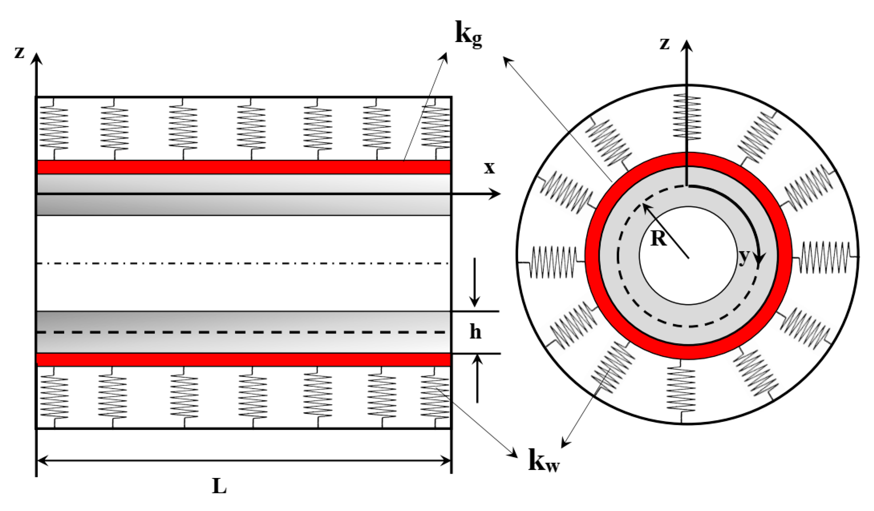
2. Governing Equations of the Problem

Let us consider a BD-FG porous cylindrical shell embedded in an elastic foundation with thickness $h$, radius $R$, and length $L$, where two different porosity distributions of the constituent phases are accounted for the analysis, namely an even and an uneven distribution, see Figure 1 and Figure 2. We assume a BD-FG material made of a metal (labeled as $m$) and a ceramic (labeled as $c$) in the inner and outer shell surfaces, respectively. While the material properties for a conventional FG model vary continuously along the thickness direction from a ceramic or metal to another one, the basic material properties selected herein, vary also along the shell length from the metal to the ceramic phase. To this end, the volume fractions of the ceramic and metal phases are defined as follows

$$V_c\left(x,z\right)={\left(\frac{1}{2}+\frac{z}{h}\right)}^{n_z}{\left(\frac{x}{L}\right)}^{n_x}, V_m\left(x,z\right)=1-V_c\left(x,z\right),$$

(1)

where $n_z$ and $n_x$ refer to the non-negative volume fraction exponents defining the profile variation of the material properties along the shell thickness and length directions, respectively. In addition, z and x stand for the radial distance from the mid-plane and longitudinal distance from the origin of the BD-FG cylindrical shell, respectively. The effective material properties (i.e., Yong’s modulus, density and Poisson’s ratio) of the BD-FG porous cylindrical shell are assumed to change according to a modified power law model with a linear algebraic combination of volume fractions of two basic materials. Two types of BD-FG material models include both even and/or uneven porosity distributions, i.e.,

$$E\left(x,z\right)=E_m+\left(E_c-E_m\right){\left(\frac{1}{2}+\frac{z}{h}\right)}^{n_z}{\left(\frac{x}{L}\right)}^{n_x}-\frac{\zeta }{2}\left(E_c+E_m\right),$$

(2a)

$$\rho \left(x,z\right)={\rho }_m+\left({\rho }_c-{\rho }_m\right){\left(\frac{1}{2}+\frac{z}{h}\right)}^{n_z}{\left(\frac{x}{L}\right)}^{n_x}-\frac{\zeta }{2}\left({\rho }_c+{\rho }_m\right),$$

(2b)

$$\nu \left(x,z\right)={\nu }_m+\left({\nu }_c-{\nu }_m\right){\left(\frac{1}{2}+\frac{z}{h}\right)}^{n_z}{\left(\frac{x}{L}\right)}^{n_x}-\frac{\zeta }{2}\left({\nu }_c+{\nu }_m\right),$$

(2c)

for even distributions, or

$$E\left(x,z\right)=E_m+\left(E_c-E_m\right){\left(\frac{1}{2}+\frac{z}{h}\right)}^{n_z}{\left(\frac{x}{L}\right)}^{n_x}-\frac{\xi }{2}\left(E_c+E_m\right)\left(1+\frac{2\left|z\right|}{h}\right),$$

(3a)

$$\rho \left(x,z\right)={\rho }_m+\left({\rho }_c-{\rho }_m\right){\left(\frac{1}{2}+\frac{z}{h}\right)}^{n_z}{\left(\frac{x}{L}\right)}^{n_x}-\frac{\xi }{2}\left({\rho }_c+{\rho }_m\right)\left(1+\frac{2\left|z\right|}{h}\right),$$

(3b)

$$\nu \left(x,z\right)={\nu }_m+\left({\nu }_c-{\nu }_m\right){\left(\frac{1}{2}+\frac{z}{h}\right)}^{n_z}{\left(\frac{x}{L}\right)}^{n_x}-\frac{\xi }{2}\left({\nu }_c+{\nu }_m\right)\left(1+\frac{2\left|z\right|}{h}\right),$$

(3c)

for an uneven distribution. In the all the expression (2) and (3), $\zeta$ and $\xi$ denote the volume fraction of an even or uneven porosity inside the phases, respectively. While an even model accounts for porosities evenly distributed across the radial direction, the porosities in an uneven model is mostly concentrated in the shell mid-plane. It is worth noting that the uneven porosity distribution is linearly reduced from a larger value at mid-plane to a smaller value at the top and bottom sides of the structure.

In what follows, we apply the TSDT, such that the displacement field of an arbitrary point of the shell along the $x$, $y$, and $z$ axes, is defined as

$$\begin{gathered} u\left(x,y,z,t\right)=u_0\left(x,y,t\right)+z{\phi }_x\left(x,y,t\right)-\overline{c}{z}^3\left({\phi }_x\left(x,y,t\right)+\frac{\partial w_0\left(x,y,t\right)}{\partial x}\right), \\ v\left(x,y,z,t\right)=v_0\left(x,y,t\right)+z{\phi }_y\left(x,y,t\right)-\overline{c}{z}^3\left({\phi }_y\left(x,y,t\right)+\frac{\partial w_0\left(x,y,t\right)}{\partial y}\right), \\ w\left(x,y,z,t\right)=w_0\left(x,y,t\right), \end{gathered}$$

(4)

where $\overline{c}=\frac{4}{3h^2}$, and $u$, $v$, $w$ stand for the longitudinal, circumferential, and transverse (radial) displacement components, respectively. These are determined, in turn, by means of the kinematic quantities $u_0$, $v_0$, and $w_0$ at the middle surface, and the rotations ${\phi }_x$ and ${\phi }_y$ of a transverse normal section about the $x$ and $y$ axis, respectively.

According to the TSDT, the strain components of the cylindrical shell can be written as [48]

$${\epsilon }_{xx}=\frac{\partial u_0\left(x,y,t\right)}{\partial x}+z\frac{\partial {\phi }_x\left(x,y,t\right)}{\partial x}-\overline{c}{z}^3\left(\frac{\partial {\phi }_x\left(x,y,t\right)}{\partial x}+\frac{{\partial }^2{w}_0\left(x,y,t\right)}{\partial x^2}\right),$$

(5a)

$${\epsilon }_{yy}=\frac{\partial v_0\left(x,y,t\right)}{\partial y}+z\frac{\partial {\phi }_y\left(x,y,t\right)}{\partial y}-\overline{c}{z}^3\left(\frac{\partial {\phi }_y\left(x,y,t\right)}{\partial y}+\frac{{\partial }^2{w}_0\left(x,y,t\right)}{\partial y^2}\right)+\frac{w}{R},$$

(5b)

$$\begin{array}{l}{\gamma }_{xy}=\frac{\partial u_0\left(x,y,t\right)}{\partial y}+\frac{\partial v_0\left(x,y,t\right)}{\partial x}+z\left(\frac{\partial {\phi }_x\left(x,y,t\right)}{\partial y}+\frac{\partial {\phi }_y\left(x,y,t\right)}{\partial x}\right)\\ -\overline{c}{z}^3\left(\frac{\partial {\phi }_x\left(x,y,t\right)}{\partial y}+\frac{\partial {\phi }_y\left(x,y,t\right)}{\partial x}+2\frac{{\partial }^2{w}_0\left(x,y,t\right)}{\partial y\partial x}\right),\end{array}$$

(5c)

$${\gamma }_{xz}={\phi }_x\left(x,y,t\right)-2\overline{c}{z}^2\left({\phi }_x\left(x,y,t\right)+\frac{\partial w_0\left(x,y,t\right)}{\partial x}\right)+\frac{\partial w_0\left(x,y,t\right)}{\partial x},$$

(5d)

$${\gamma }_{yz}={\phi }_y\left(x,y,t\right)-2\overline{c}{z}^2\left({\phi }_y\left(x,y,t\right)+\frac{\partial w_0\left(x,y,t\right)}{\partial y}\right)+\frac{\partial w_0\left(x,y,t\right)}{\partial y},$$

(5e)

which are related to the stress components as follows

$$\left\{\begin{array}{l}{\sigma }_{xx}\\ {\sigma }_{yy}\\ {\sigma }_{xz}\\ {\sigma }_{yz}\\ {\sigma }_{xy}\end{array}\right\}=\left[\begin{array}{ccccc}{Q}_{11}& Q_{12}& 0& 0& 0\\ Q_{21}& Q_{22}& 0& 0& 0\\ 0& 0& Q_{44}& 0& 0\\ 0& 0& 0& Q_{55}& 0\\ 0& 0& 0& 0& Q_{66}\end{array}\right]\left\{\begin{array}{l}{\epsilon }_{xx}\\ {\epsilon }_{yy}\\ {\epsilon }_{xz}\\ {\epsilon }_{yz}\\ {\epsilon }_{xy}\end{array}\right\},$$

(6)

where the stiffness $Q_{ij}$ is defined as

$$\begin{gathered} Q_{11}\left(x,z\right)=Q_{22}\left(x,z\right)=\frac{E\left(x,z\right)}{1-{\left(\nu \left(x,z\right)\right)}^2}, Q_{12}\left(x,z\right)=Q_{21}\left(x,z\right)=\nu \left(x,z\right)Q_{11}\left(x,z\right), \\ {Q}_{44}\left(x,z\right)=Q_{55}\left(x,z\right)=Q_{66}\left(x,z\right)=\frac{E\left(x,z\right)}{2\left(1+\nu \left(x,z\right)\right)}. \end{gathered}$$

(7)

The strain energy of the BD-FG porous cylindrical shell is expressed as follow

$${\Pi }_S=\frac{1}{2}{\displaystyle \underset{0}{\overset{L}{\int }}{\displaystyle \underset{0}{\overset{2\pi R}{\int }}{\displaystyle \underset{-\frac{h}{2}}{\overset{\frac{h}{2}}{\int }}({\sigma }_{xx}{\epsilon }_{xx}+}}}{\sigma }_{yy}{\epsilon }_{yy}+{\tau }_{xy}{\gamma }_{xy}+{\tau }_{xz}{\gamma }_{xz}+{\tau }_{yz}{\gamma }_{yz})dzdydx,$$

(8)

and the kinetic energy of the cylindrical shell reads

$${\Pi }_T=\frac{1}{2}{\displaystyle \underset{0}{\overset{L}{\int }}{\displaystyle \underset{0}{\overset{2\pi R}{\int }}{\displaystyle \underset{-\frac{h}{2}}{\overset{\frac{h}{2}}{\int }}\rho \left(x,z\right)({\left(\frac{\partial u\left(x,y,z,t\right)}{\partial t}\right)}^2}}}+{\left(\frac{\partial v\left(x,y,z,t\right)}{\partial t}\right)}^2+{\left(\frac{\partial w\left(x,y,z,t\right)}{\partial t}\right)}^2)dzdydx.$$

(9)

The total potential energy corresponding to the axial compressive load $F_a(t)$ together with the Winkler and/or Pasternak elastic foundation, can be written as follow

$${\Pi }_E=\frac{1}{2}{\displaystyle \underset{0}{\overset{L}{\int }}{\displaystyle \underset{0}{\overset{2\pi R}{\int }}{\displaystyle \underset{-\frac{h}{2}}{\overset{\frac{h}{2}}{\int }}(k_w{w}_{{}_0}{}^2+}}}{k}_g\left({\left(\frac{\partial w_0}{\partial x}\right)}^2+{\left(\frac{\partial w_0}{\partial y}\right)}^2\right)+F_a\left(t\right){\left(\frac{\partial w_0}{\partial x}\right)}^2)dzdydx,$$

(10)

where $k_w$ and $k_g$ refer to the Winkler foundation stiffness and shear layer stiffness of the elastic foundation, respectively.

Consistently with the Hamilton’s principle, the following governing equations of motion for the BD-FG cylindrical shell are determined

$${\displaystyle \underset{t_1}{\overset{t_2}{\int }}\left(\delta {\Pi }_T-\delta {\Pi }_S-\delta {\Pi }_E\right)dt=0},$$

(11)

where the symbol $\delta$ denotes the variation of the energy quantities. By combination of Equations (8)–(10) and Equation (11), after integration by parts, we get the following governing equations of motion, under the assumption of a null value for $u_0$, $v_0$, $w_0$, ${\phi }_x$, and ${\phi }_y$.

$$\frac{\partial N_{xx}}{\partial x}+\frac{\partial N_{xy}}{\partial y}=I_0\left(x\right)\frac{{\partial }^2{u}_0\left(x,y,t\right)}{\partial t^2}+\left(I_0\left(x\right)-\overline{c}{I}_3\left(x\right)\right)\frac{{\partial }^2{\phi }_x\left(x,y,t\right)}{\partial t^2}-\overline{c}{I}_3\left(x\right)\frac{{\partial }^3{w}_0}{\partial x\partial t^2},$$

(12a)

$$\frac{\partial N_{xy}}{\partial y}+\frac{\partial N_y}{\partial y}=I_0\left(x\right)\frac{{\partial }^2{v}_0\left(x,y,t\right)}{\partial t^2}+\left(I_0\left(x\right)-\overline{c}{I}_3\left(x\right)\right)\frac{{\partial }^2{\phi }_y\left(x,y,t\right)}{\partial t^2}-\overline{c}{I}_3\left(x\right)\frac{{\partial }^3{w}_0\left(x,y,t\right)}{\partial y\partial t^2},$$

(12b)

$$\begin{array}{l}\frac{\partial Q_{xz}}{\partial x}+\frac{\partial Q_{xy}}{\partial y}-3\overline{c}\left(\frac{\partial R_{xz}}{\partial x}+\frac{\partial R_{xy}}{\partial y}\right)+\overline{c}(\frac{{\partial }^2{P}_{xx}}{\partial x^2}+2\frac{{\partial }^2{P}_{xy}}{\partial x\partial y}+\frac{{\partial }^2{P}_{yy}}{\partial y^2})-\frac{N_{yy}}{R}\\ -k_w{w}_0\left(x,y,t\right)+k_g\left(\frac{{\partial }^2{w}_0\left(x,y,t\right)}{\partial x^2}+\frac{{\partial }^2{w}_0\left(x,y,t\right)}{\partial y^2}\right)+F_a\frac{{\partial }^2{w}_0\left(x,y,t\right)}{\partial x^2}=I_0\left(x\right)\frac{{\partial }^2{w}_0\left(x,y,t\right)}{\partial t^2}\\ -{\overline{c}}^2{I}_6\left(x\right)\left(\frac{{\partial }^4{w}_0\left(x,y,t\right)}{\partial x^2\partial t^2}+\frac{{\partial }^4{w}_0\left(x,y,t\right)}{\partial y^2\partial t^2}\right)+\overline{c}{I}_3\left(x\right)\left(\frac{{\partial }^3{u}_0\left(x,y,t\right)}{\partial x\partial t^2}+\frac{{\partial }^3{v}_0\left(x,y,t\right)}{\partial y\partial t^2}\right)\\ +\overline{c}\left(I_4\left(x\right)-\overline{c}{I}_6\left(x\right)\right)\left(\frac{{\partial }^3{\phi }_x\left(x,y,t\right)}{\partial x\partial t^2}+\frac{{\partial }^3{\phi }_y\left(x,y,t\right)}{\partial y\partial t^2}\right),\end{array}$$

(12c)

$$\begin{array}{l}\frac{\partial M_{xx}}{\partial x}+\frac{\partial M_{xy}}{\partial y}-Q_{xz}+3\overline{c}{R}_{xz}-\overline{c}\left(\frac{\partial P_{xx}}{\partial x}+\frac{\partial P_{xy}}{\partial y}\right)=\left(I_0\left(x\right)-\overline{c}{I}_3\left(x\right)\right)\frac{{\partial }^2{u}_0\left(x,y,t\right)}{\partial t^2}\\ +\left(I_2\left(x\right)-2\overline{c}{I}_4\left(x\right)+{\overline{c}}^2{I}_6\left(x\right)\right)\frac{{\partial }^2{\phi }_x\left(x,y,t\right)}{\partial t^2}\\ -\overline{c}\left(I_4\left(x\right)-\overline{c}{I}_6\left(x\right)\right)\frac{{\partial }^3{w}_0\left(x,y,t\right)}{\partial x\partial t^2},\end{array}$$

(12d)

$$\begin{array}{l}\frac{\partial M_{yy}}{\partial y}+\frac{\partial M_{xy}}{\partial x}-Q_{yz}+3\overline{c}{R}_{yz}-\overline{c}\left(\frac{\partial P_{yy}}{\partial y}+\frac{\partial P_{xy}}{\partial x}\right)=\left(I_0\left(x\right)-\overline{c}{I}_3\left(x\right)\right)\frac{{\partial }^2{v}_0\left(x,y,t\right)}{\partial t^2}\\ +\left(I_2\left(x\right)-2\overline{c}{I}_4\left(x\right)+{\overline{c}}^2{I}_6\left(x\right)\right)\frac{{\partial }^2{\phi }_y\left(x,y,t\right)}{\partial t^2}\\ -\overline{c}\left(I_4\left(x\right)-\overline{c}{I}_6\left(x\right)\right)\frac{{\partial }^3{w}_0\left(x,y,t\right)}{\partial y\partial t^2},\end{array}$$

(12e)

Note that the resultants in Equation (12) are computed by integration of the pertaining stress components along the shell structure, i.e.,

$$\left\{\begin{array}{l}{N}_{xx}\\ N_{yy}\\ N_{xy}\end{array}\right\}={\displaystyle \underset{-\frac{h}{2}}{\overset{\frac{h}{2}}{\int }}\left\{\begin{array}{l}{\sigma }_{xx}\\ {\sigma }_{yy}\\ {\tau }_{xy}\end{array}\right\}dz},$$

(13)

$$\left\{\begin{array}{l}{M}_{xx}\\ M_{yy}\\ M_{xy}\end{array}\right\}={\displaystyle \underset{-\frac{h}{2}}{\overset{\frac{h}{2}}{\int }}\left\{\begin{array}{l}{\sigma }_{xx}\\ {\sigma }_{yy}\\ {\tau }_{xy}\end{array}\right\}zdz},$$

(14)

$$\left\{\begin{array}{l}{P}_{xx}\\ P_{yy}\\ P_{xy}\end{array}\right\}={\displaystyle \underset{-\frac{h}{2}}{\overset{\frac{h}{2}}{\int }}\left\{\begin{array}{l}{\sigma }_{xx}\\ {\sigma }_{yy}\\ {\tau }_{xy}\end{array}\right\}{z}^{3}dz},$$

(15)

$$\left\{\begin{array}{l}{Q}_{xz}\\ Q_{yz}\end{array}\right\}={\displaystyle \underset{-\frac{h}{2}}{\overset{\frac{h}{2}}{\int }}\left\{\begin{array}{l}{\tau }_{xz}\\ {\tau }_{yz}\end{array}\right\}dz},$$

(16)

$$\left\{\begin{array}{l}{R}_{xz}\\ R_{yz}\end{array}\right\}={\displaystyle \underset{-\frac{h}{2}}{\overset{\frac{h}{2}}{\int }}\left\{\begin{array}{l}{\tau }_{xz}\\ {\tau }_{yz}\end{array}\right\}{z}^{2}dz}.$$

(17)

The generalized inertia moments are defined as

$$\left(I_0\left(x\right),I_1\left(x\right),I_2\left(x\right),I_4\left(x\right),I_5\left(x\right),I_6\left(x\right)\right)={\displaystyle \underset{-\frac{h}{2}}{\overset{\frac{h}{2}}{\int }}\left(1,z,z^2,z^3,z^4,z^6\right)}\rho \left(x,z\right)dz.$$

(18)

Three types of boundary conditions are considered along the shell edges, namely

➢

Simply-Simply (S-S) supports

$$x=0,L\Rightarrow v_0=w_0={\phi }_y=M_x=N_x=0,$$

(19)

➢

Clamped-Clamped (C-C) supports

$$x=0,L\Rightarrow u_0=v_0=w_0={\phi }_x={\phi }_y=0,$$

(20)

➢

Clamped-simply (C-S) supports

$$x=0\Rightarrow u_0=v_0=w_0={\phi }_x={\phi }_y=0,$$

(21a)

$$x=L\Rightarrow v_0=w_0={\phi }_y=M_x=N_x=0,$$

(21b)

3. Solution Procedure

In this section, we want to determine the dynamic stability of BD-FG porous cylindrical shells, where the governing equations of motion are expressed through the following expansion for the kinematic quantities

$$u_0\left(x,y,t\right)=U\left(x\right)\sin \left(n\frac{y}{R}\right)\overline{U}\left(t\right)$$

(22a)

$$v_0\left(x,y,t\right)=V\left(x\right)\cos \left(n\frac{y}{R}\right)\overline{V}\left(t\right)$$

(22b)

$$w_0\left(x,y,t\right)=W\left(x\right)\sin \left(n\frac{y}{R}\right)\overline{W}\left(t\right)$$

(22c)

$${\phi }_x\left(x,y,t\right)={\Phi }_x\left(x\right)\sin \left(n\frac{y}{R}\right){\overline{\Phi }}_x\left(t\right)$$

(22d)

$${\phi }_y\left(x,y,t\right)={\Phi }_y\left(x\right)\cos \left(n\frac{y}{R}\right){\overline{\Phi }}_y\left(t\right)$$

(22e)

where n is the circumferential half wave number, $\overline{U}\left(t\right)$, $\overline{V}\left(t\right)$, $\overline{W}\left(t\right)$, ${\overline{\Phi }}_x\left(t\right)$ and ${\overline{\Phi }}_y\left(t\right)$ are the time functions. The admissible displacement functions in Equation (22) satisfy both the equations of motion and their boundary conditions. Afterward, the governing equations of the problem are discretized according to the GDQ method.

Upon substitution of Equation (22a–e) and Equation (5a–e) into Equation (12), after a proper manipulation, we obtain the equations of motion in their final form, as detailed in Appendix A.

The above-mentioned equations of motion are solved numerically in a strong form by means of the GDQ method, as largely discussed in [49] and in a review paper [50] in terms of accuracy, stability and reliability, and successfully applied for many numerical applications, namely, the buckling, free vibration, or dynamic problems of composite structures [51,52,53,54,55], as well as the fracture mechanics problems [56,57] or non-linear transient problems [58,59]. In addition, the Bolotin method [60] is proposed herein to determine the DIRs for the differential equations system, known as Mathieu–Hill system of equations. More details about the basics of the proposed numerical tools are recalled in what follows.

3.1. The GDQ Method

The GDQ method approximates the fundamental system of differential equations, by discretizing the derivatives of a function $J\left(x\right)$ respect to a spatial variable at a given discrete grid distribution, by means of the weighting coefficients. For a one-dimensional problem where the whole domain $0\le x\le L$ is discretized in $N$ grids points, the approximation of the nth-order derivatives of J function respect to x variable can be expressed as [49]

$$\frac{d^{n}J\left(x_p\right)}{d{x}^n}={\displaystyle \sum _{r=1}^N{\chi }_{pr}^{\left(n\right)}J\left(x_r\right)}\hspace{1em}\hspace{1em}n=1,2,\dots ,N-1,$$

(29)

${\chi }_{pr}^{\left(n\right)}$ being the weighting coefficients, defined as follows [49]

$${\chi }_{pq}^{\left(1\right)}=\frac{\mathsf{\Upsilon }\left(x_p\right)}{\left(x_p-x_q\right)\mathsf{\Upsilon }\left(x_q\right)},\hspace{1em}\hspace{1em}p\ne q;p,q=1,2,\dots ,N$$

(30)

and $\mathsf{\Upsilon }\left(x_p\right)$ is the Lagrangian operator expressed as [49]

$$\mathsf{\Upsilon }\left(x_p\right)={\displaystyle \prod _{p\ne q,q=1}^N\left(x_p-x_q\right)}.$$

(31)

For higher order derivatives of the weighting coefficients it is [49]

$${\chi }_{pq}^{\left(n\right)}=n\left({\chi }_{pp}^{\left(n-1\right)}{\chi }_{pq}^{\left(1\right)}-\frac{{\chi }_{pq}^{\left(n-1\right)}}{\left(x_p-x_q\right)}\right)$$

(32)

It is well known in literature that the type of grid distribution within the domain can affect significantly the accuracy of the proposed method [50]. In what follows we apply a Chebyshev–Gauss–Lobatto non-uniform pattern, due to its great performances, as verified by Shu [49]

$$x_p=\frac{L}{2}\left(1-\cos \left(\frac{x_p-1}{N-1}\right)\pi \right)\hspace{1em}\hspace{1em}p=1,2,\dots ,N.$$

(33)

Thus, the governing differential equations of motion and boundary conditions are discretized according to the GDQ approach, as detailed in Appendix B. Let us denote the periodic axial compressive load as

$$F_a\left(t\right)=\alpha F_{cr}+\beta F_{cr}\cos \left(\omega t\right)$$

(34)

where $\alpha$ and $\beta$ refer to the static and dynamic load factors, respectively. Furthermore, $F_{cr}$ denotes the critical static load and $\omega$ stands for the excitation frequency. By substituting Equation (34) into the third Equation (A3) from the Appendix A, and by combining the discretized equations of motion along with the associated boundary conditions, the problem can be redefined in the following matrix form

$$\left(\begin{array}{cc}{M}_{bb}& M_{bd}\\ M_{db}& M_{dd}\end{array}\right)\left\{\begin{array}{l}{\ddot{\Gamma }}_b\\ {\ddot{\Gamma }}_d\end{array}\right\}+\left(\left(\begin{array}{cc}{K}_{bb}& K_{bd}\\ K_{db}& K_{dd}\end{array}\right)+F_{cr}\left(\alpha +\beta \cos \left(\omega t\right)\right)\left(\begin{array}{cc}{K}_{bb}^G& K_{bd}^G\\ K_{db}^G& K_{dd}^G\end{array}\right)\right)\left\{\begin{array}{l}{\Gamma }_b\\ {\Gamma }_d\end{array}\right\}=\left(\begin{array}{l}0\\ 0\end{array}\right)$$

(35)

where $M$, $K$, and $K^G$ are the mass, stiffness, and geometric stiffness matrixes, respectively, and $\Gamma ={\left\{\overline{U},\overline{V},\overline{W},{\overline{\Phi }}_x,{\overline{\Phi }}_y\right\}}^T$ denotes the unknown dynamic displacement vector. In addition, indexes $b$ and $d$ indicate the boundary points and domain points, respectively.

3.2. Bolotin Method

The second order system of differential Equation (35) is known in literature as Mathieu–Hill system of equations due to presence of the periodic coefficient, accordingly. In the present study we propose the Bolotin method [60] to define the boundaries associated to the DIR of the BD-FG porous cylindrical shell. Based on this method, the dynamic displacement vector Γ can be defined in a Fourier series as follows [60]

$$\{\Gamma \}={\displaystyle \sum _{s=1,3,\dots }^{\infty }\left(\left\{{\vartheta }_s\right\}\sin \left(\frac{s\omega t}{2}\right)+\left\{{\upsilon }_s\right\}\cos \left(\frac{s\omega t}{2}\right)\right)},$$

(36)

where ${\vartheta }_s$ and ${\upsilon }_s$ denote the arbitrary time invariant vectors. It should be mentioned that the first DIR with period $2T$ is generally much meaningful and wider than the secondary one with period $T$. For this reason, in this work we consider the solutions with period $2T$. By substitution of Equation (36) into Equation (35) and by mathematical manipulation, we get the following first order equation

$$\left|\left[K\right]-F_{cr}\left(\alpha \pm \frac{\beta }{2}\right)\left[K^G\right]-\frac{{\omega }^2}{4}\left[M\right]\right|=0,$$

(37)

which represents a classical eigenvalue problem. The critical buckling load can be computed from Equation (35) by neglecting the inertia terms and by setting $\alpha +\beta \cos \left(\omega t\right)=1$. Then, solving Equation (37) for some fixed values of $\alpha$ and $F_{cr}$, the variation of the excitation frequency $\omega$ in regards to $\beta$ can be drawn as DIR for the BD-FG structure.

4. Numerical Investigation

In this section some illustrative example are shown, starting with a preliminary validation of the proposed method with respect to the available literature, and continuing with a parametric investigation of the problem, whose results are evaluated comparatively in order to evaluate the sensitivity of the mechanical response.

4.1. Validation

Due to the general lack of works in the literature on the dynamic buckling behavior of BD-FG porous cylindrical shells, the proposed model is validated, herein, for an axial buckling problem of a simply supported conventional FG cylindrical shell based on two different theories. Thus, for comparative purposes, we select the same material properties and shell geometry as reported in [48,61], and neglect the inertia terms, foundation parameters and porosity effects, while assuming a null value for $n_x$. In

Table 1. Comparative evaluation of the critical axial buckling load (MN) for a FG cylindrical shell with $h=0.001 \mathrm{m},$ $L/R=0.5,$ $E_c=380 \mathrm{GPa},$ $E_m=70 \mathrm{GPa},$ $\nu =0.3,$ $n_x=0$.

R/h		Khazaeinejad and Najafizadeh [61]	Present
5	Alumina	1.598 (1,1)	1.5975
	nz = 1	0.853 (1,1)	0.8532
	nz = 2	0.662 (1,1)	0.6624
	nz = 5	0.520 (1,1)	0.5197
	nz = 10	0.450 (1,1)	0.4500
	Aluminum	0.294 (1,1)	0.2942
10	Alumina	1.403 (1,1)	1.4029
	nz = 1	0.759 (1,1)	0.7589
	nz = 2	0.589 (1,1)	0.5885
	nz = 5	0.456 (1,1)	0.4557
	nz = 10	0.393 (1,1)	0.3931
	Aluminum	0.258 (1,1)	0.2584
20	Alumina	1.594 (1,1)	1.5936
	nz = 1	0.903 (1,1)	0.9029
	nz = 2	0.698 (1,1)	0.6977
	nz = 5	0.514 (1,1)	0.5140
	nz = 10	0.430 (1,1)	0.4295
	Aluminum	0.293 (1,1)	0.2935
30	Alumina	1.566 (2,1)	1.5664
	nz = 1	0.826 (2,1)	0.8262
	nz = 2	0.642 (2,1)	0.6419
	nz = 5	0.511 (2,1)	0.5108
	nz = 10	0.449 (2,1)	0.4486
	Aluminum	0.289 (2,1)	0.2885
100	Alumina	1.443 (3,1)	1.4428
	nz = 1	0.782 (3,1)	0.7822
	nz = 2	0.606 (3,1)	0.6064
	nz = 5	0.469 (3,1)	0.4681
	nz = 10	0.404 (3,1)	0.4008
	Aluminum	0.266 (3,1)	0.2657
300	Alumina	1.443 (5,1)	1.4431
	nz = 1	0.787 (5,1)	0.7841
	nz = 2	0.610 (5,1)	0.6079
	nz = 5	0.468 (5,1)	0.4683
	nz = 10	0.402 (5,1)	0.4017
	Aluminum	0.266 (5,1)	0.2658

we summarize the results in terms of critical axial buckling load $F_{cr}$ for a FG cylindrical shell with $h=0.001 \mathrm{m}$, $L/R=0.5$, $E_c=380 \mathrm{G}\mathrm{P}\mathrm{a}$, $E_m=70 \mathrm{G}\mathrm{P}\mathrm{a}$, $\nu =0.3$, $\overline{c}=0$, with a clear excellent agreement between our results and predictions in Ref. [61] based on the first order shear deformation theory. This first numerical example could be considered as limit case, where the TSDT reverts to the FSDT, since it refers to a thin shell structure, just for validation purposes. More accurate results, however, are always expected under a TSDT assumption for increased values of the shell thickness, as done in the next parametric investigation.

As further comparative study,

Table 2. Comparative evaluation of the dimensionless critical axial buckling load for a FG cylindrical shell with $h=0.001 \mathrm{m},$ $E_m=70 \mathrm{GPa},$ $\nu =0.3,$ $n_z=2$.

Z	h/R	Bagherizadeh et al. [48]	Present
50	0.01	79.9296 (4,5)	79.9295
	0.025	79.48684 (4,3)	79.4868
	0.05	78.79842 (4,3)	78.7984
300	0.01	479.5066 (10,5)	479.5065
	0.025	476.3834 (10,3)	476.3834
	0.05	470.8775 (11,1)	470.8775
900	0.01	1438.157 (18,3)	1438.1576
	0.025	1428.611 (18,2)	1428.6108
	0.05	1412.380 (19,1)	1412.3802

compares the dimensionless critical buckling load ($P_{cr}=F_{cr}{L}^2/{\pi }^2{D}_m$; $D_m=E_m{h}^3/12\left(1-{\nu }_m^2\right)$) for a FG cylindrical shell with $h=0.001 \mathrm{m}$, $E_c=380 \mathrm{G}\mathrm{P}\mathrm{a}$, $E_m=70 \mathrm{G}\mathrm{P}\mathrm{a}$, $\nu =0.3$, $\overline{c}=4/3h^2$. Based on Table 2, it is worth noticing the high precision between our results and predictions by Bagherizadeh et al. [48], which confirms the accuracy of the GDQ method. This method is thus proposed in the following parametric study, as efficient numerical tool to solve the problem.

4.2. Parametric Study

We refer to a BD-FG cylindrical structure with constituent phases of properties listed in

Table 3. Material properties of the BD-FG cylindrical shell.

Constituent Phases	Materi	Properties
		E (GPa)	ρ (Kg/m3)	ν
c	SiC	427	3100	0.17
m	Al	70	2702	0.3

, where the following dimensionless parameters are considered to compute the dimensionless structural excitation frequencies

$$\Omega =\omega R\sqrt{\frac{{\rho }_m}{E_m}}, K_g=\frac{k_g{R}^2}{E_m{h}^3}, K_w=\frac{k_w{R}^4}{E_m{h}^3}.$$

(38)

We determine the DIR, and highlight the effects of different parameters such as the thickness-to-radius ratio ($h/R$), the length-to-radius ratio ($L/R$), the static load factor, the boundary conditions, the power law indexes ($n_x$,$n_z$), the type and volume fraction of porosity, and the foundation parameters, on the dynamic buckling behavior of the BD-FG cylindrical shell.

In Figure 3 we plot the variation of the DIR for different thickness-to-radius ratios ($h/R$), where a clear shift of the DIR is observed for increasing $h/R$ ratios. This means that the DIR becomes wider for a certain value of the dynamic load factor, and occurs with a sort of delay. An increased $h/R$ ratio from 0.01 to 0.1 yields a global shift of the DIR origin point towards high excitation frequencies.

Figure 4 shows the sensitivity of the DIR for varying $L/R$ ratios, while keeping fixed $h/R=0.01$. In detail, for $L/R=1$ the structure has a wider DIR in comparison with the other values, whereby an increasing $L/R$ ratio yields the DIR to take place at lower excitation frequencies. Based on the plots in Figure 4, we can observe a reduction of about 41.96% in the excitation frequencies corresponding to the origin of the instability region, for a $L/R$ ranging between 1 and 10. When the $L/R$ ratio features higher magnitudes, the bending resistance gradually reduces and yields an increased bending deformation.

In Figure 5, we evaluate the effect of the static load factor on the instability region of the BD-FG cylindrical shell. As expected, in absence of a static load on the structure, the width of DIR gets smaller, whereby for an increased static load factor, it becomes gradually greater for a fixed value of dynamic load factor (i.e., $\beta =1$), and its origin tends to move on the left side. This proves the sensitivity of the structural instability to the static load factor.

As also visible in Figure 6, we evaluate the impact of different boundary conditions on the DIR of the cylindrical shell. Here, we consider three different boundary conditions, namely, S-S, C-S, and C-C boundary conditions. Based on the plots of Figure 7, it is worth noting that a C-C boundary conditions yields higher values of the dimensionless excitation frequencies than those ones provided by a S-S or C-S supports, due to an increased stiffness of the structure. Furthermore, the origin of the instability region tends to get away from the origin. Once the dynamic load factor β reaches the unit value, the width of the DIR for S-S boundary condition becomes smaller, compared to the other boundary conditions. This means that, for lower values of dimensionless excitation frequency, a BD-FG cylindrical shell with S-S supports tends to become more unstable compared to the other boundary conditions.

A further investigation is devoted to study the influence of the power law index along the length $n_x$ on the dynamic buckling behavior of one-directional FG cylindrical shell, as depicted Figure 7. In such a case, the DIR takes place at lower frequencies owning to an increased magnitude of the power law index. The effect of an increased dimensionless excitation frequency related to the origin of the DIR is meaningful within the range $0.2\le n_x\le 5$. For greater values of $n_x$, the variation in frequency corresponding to the origin of DIR becomes less remarkable. A one-directional FG cylindrical shell with $n_x=10$ or $n_x=8$ is more sensitive to the dynamic instability for lower excitation frequencies compared with those ones with $n_x\le 5$.

For a conventional FG cylindrical shell, we also investigate the effect of the transverse power index $n_z$ on the DIR, as plotted in Figure 8. It can be mentioned that for a constant value of the dynamic load factor, the enhancement of $n_z$ yields a reduction width of the dynamic instability region, especially for lower excitation frequencies. In addition, the origin DIR moves to a lower dimensionless excitation frequency. Comparing the results from Figure 7 and Figure 8, it can be concluded that, a double increase of both $n_x$, and $n_z$, leads to a reduction in the excitation frequency. Nevertheless, $n_x$ plays an important role in the reduction of the excitation frequency and in the increase of the structural instability. For $\beta =0$, for example, we note a reduction of the excitation frequency equal to 49.3% and 44.49%, for and increasing value of $n_x$ and $n_z$ from 0.2 up to 10, respectively.

Figure 9 shows the effect of the transverse and longitudinal volume fraction indexes on the DIR. In detail, for an increase of these two parameters, the origin of DIR moves to higher dimensionless excitation frequency, and the DIR width declines. In conclusion, the double increase of $n_x$ and $n_z$ leads a metal phase reinforcement, with a overall decrease of the structural stiffness and an increase in the structural instability. BD-FG cylindrical shells with lower values of $n_z$ and $n_x$, are less sensitive to the dynamic instability, due to their higher stiffness. The contrary occurs for higher values of $n_x$ and $n_z$ due to an increased deformability of the structure. The importance of applying BD-FG materials is highlighted when the variation of material properties is considered in a single direction or more directions simultaneously. This issue can be beneficial for the fabrication and design purposes of modern FG structures. Subsequently, the dynamic stability of BD-FG cylindrical shells can be controlled selecting appropriate power indexes corresponding to the desired direction.

Moreover, Figure 10 shows the effect of an even porosity volume fraction on the dimensionless excitation frequency of a BD-FG porous cylindrical shell. Note that the dimensionless excitation frequency decreases for increasing values of $n_x$ and $n_z$. In addition, for a fixed value of $n_x$, $n_z$, the excitation frequency tends to converge to a common point. As expected, at the intersection point, the effect of an even porosity volume fraction, $\zeta$, on the dimensionless excitation frequency is almost negligible. However, for different values of $n_x$, $n_z$, the effect of even porosity between the ceramic and metal phases can change significantly, such that before the intersection point, an increased even porosity volume fraction increases the dimensionless excitation frequency, and the contrary occurs after the intersection point, with a gradual decrease in the excitation frequency for an enhanced $\zeta$. The additional Figure 11 and Figure 12 show the different response for different values of $\zeta$, while assuming the same value for $n_x$ and $n_z$. In detail, under the assumption $n_x=n_z=0.15$ (Figure 11), it is visible that an increased porosity $\zeta$ moves the DIR towards higher excitation frequencies. A reversed behavior occurs in Figure 12 under the assumption $n_x=n_z=1.5$, since an increased value of $\zeta$ causes a general shift of the DIR to lower excitation frequencies. This confirms the effect of either the even porosity volume fraction $\zeta$ and the power indexes $n_x$ and $n_z$ on the stability response of the structure.

In Figure 13, Figure 14 and Figure 15 we repeat the parametric analysis to evaluate the effect of an uneven porosity between two phases of the second ceramic and second metal. In detail, Figure 13 shows the variation of the dimensionless excitation frequency versus $n_x$, $n_z$, for different values of $\xi$. Figure 14 is devoted to check for the influence of $\xi$ on the DIR of the structure for $n_x=n_z=0.15$. Additionally, in this case, we can observe as the DIR moves to the right side by increasing ξ and it takes place at higher excitation frequencies. Nevertheless, by assuming $n_x=n_z=1.5$, a different trend is noticed for the DIR in Figure 15, since an increased value of $\xi$ yields the DIR to occur at lower excitation frequencies and its width gets smaller.

The last parametric analysis considers the possible sensitivity of the response to the elastic foundation. For this reason, Figure 16 and Figure 17 plot the variation of the DIR with the Winkler or the Pasternak foundation coefficients, respectively. A noteworthy increase in stiffness emerges from both figures, where the origin of the DIR moves towards higher values of frequency. According to a comparative evaluation of the results, it seems that the best dynamic behavior of the cylindrical shell is reached for a structure surrounded by a Pasternak elastic foundation. Hence, the effect of the Pasternak elastic coefficient is more remarkable than the Winkler-based one, where a BD-FG cylindrical shell becomes more stable if embedded in a Pasternak foundation.

5. Conclusions

This work investigates the dynamic stability of BD-FG cylindrical shells embedded in an elastic foundation, including possible effects related to porosity. The material properties of BD-FG porous cylindrical shells are computed according to a modified BD power law model. Using the Hamilton’s principle, we determine the governing equations of the problem, under the classical TSDT assumptions. The aforementioned equations are rewritten into a system of Mathieu–Hill equations, according to a GDQ approach. The work is also devoted to determine the DIR of the structure while applying the Bolotin method. After a preliminary validation of the proposed formulation, with respect to the available literature, we perform a large numerical investigation to check for the sensitivity of the response both in terms of excitation frequencies and DIRs, for different thickness-to-radius ratios, length-to-radius ratios, boundary conditions, transverse and longitudinal power law indexes, even and uneven porosity volume fractions, and foundation parameters. Based on the systematic numerical investigation, the main conclusions can be summarized as follows

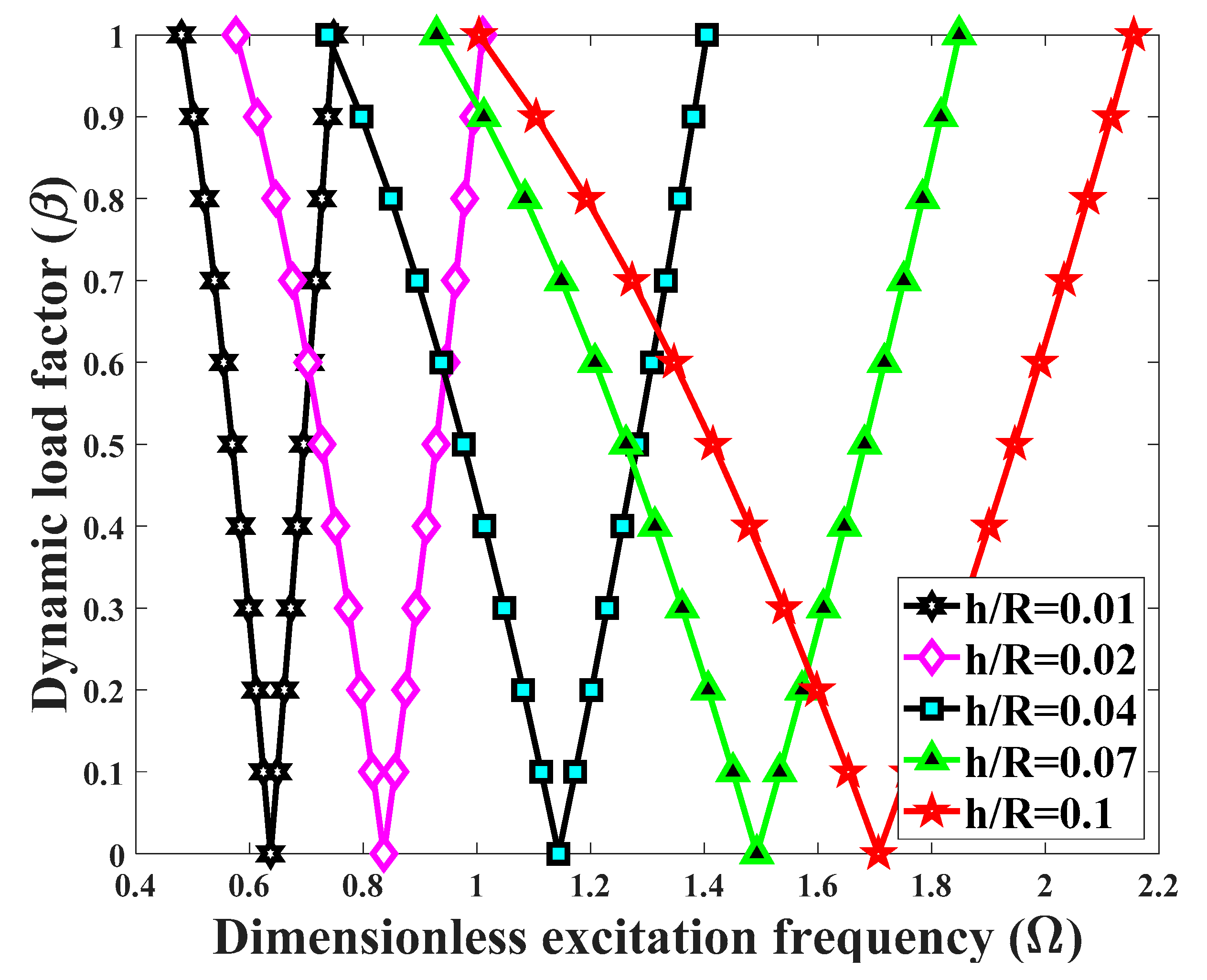
• An increased thickness-to-radius ratio causes a general shift of the DIR origin towards higher excitation frequencies. Moreover, the DIR gets wider at a certain value of the dynamic load factor.
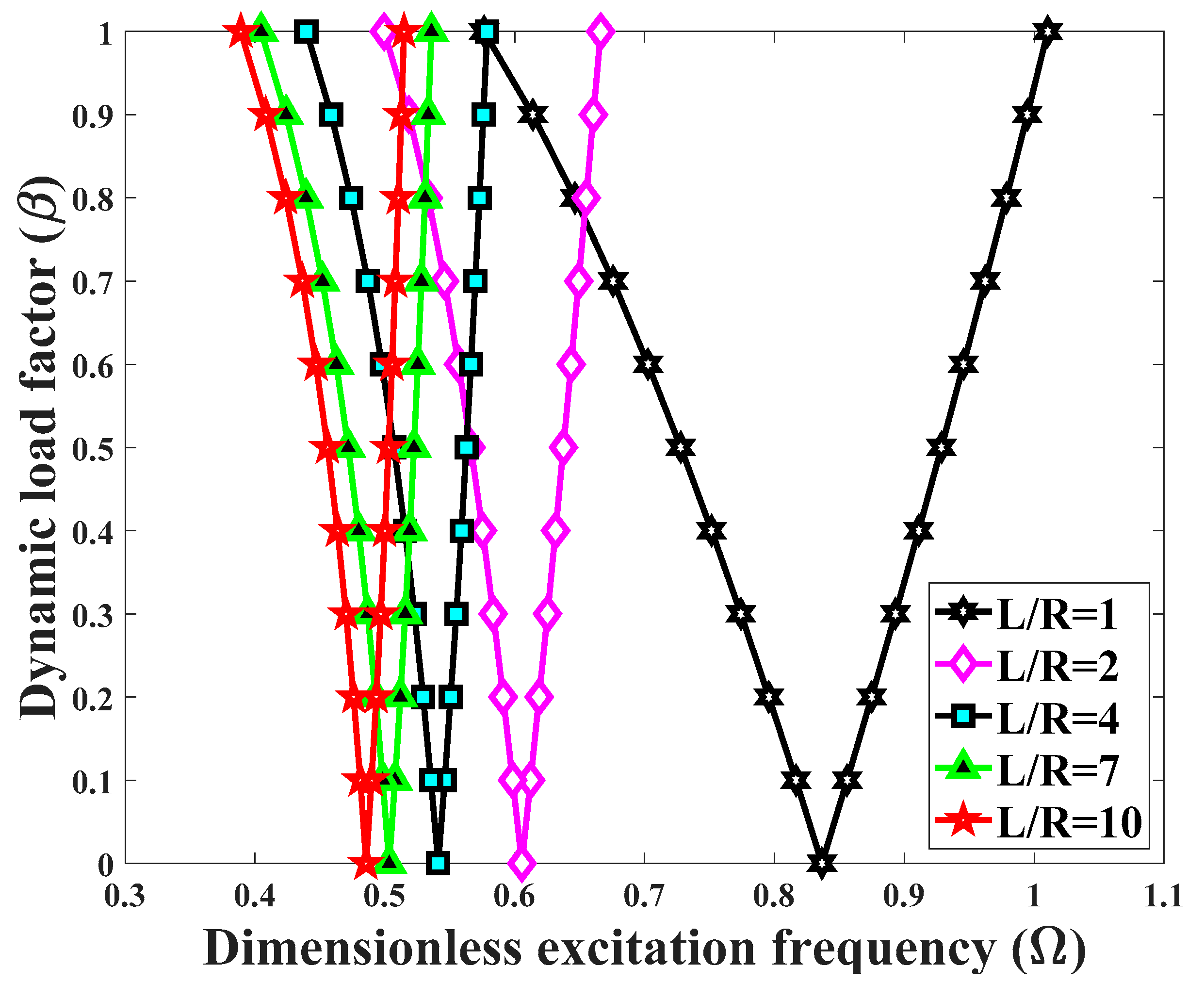
• An increased length-to-radius dimensionless ratio moves the DIR origin towards lower excitation frequencies, whereas the DIR gets smaller.
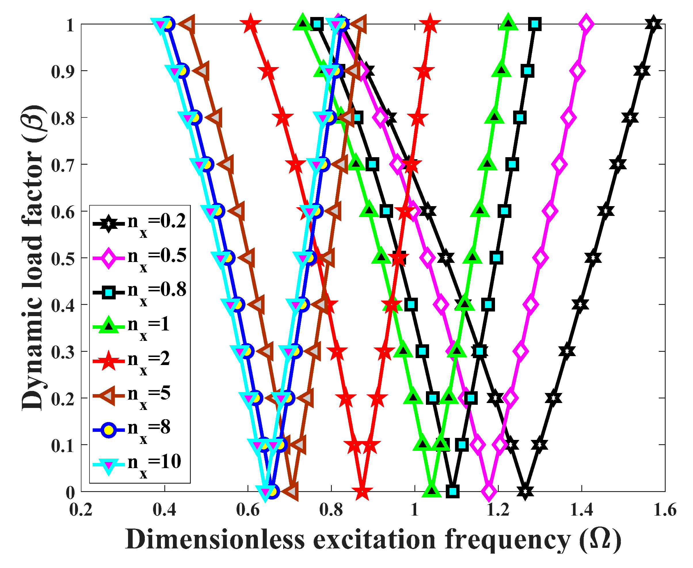
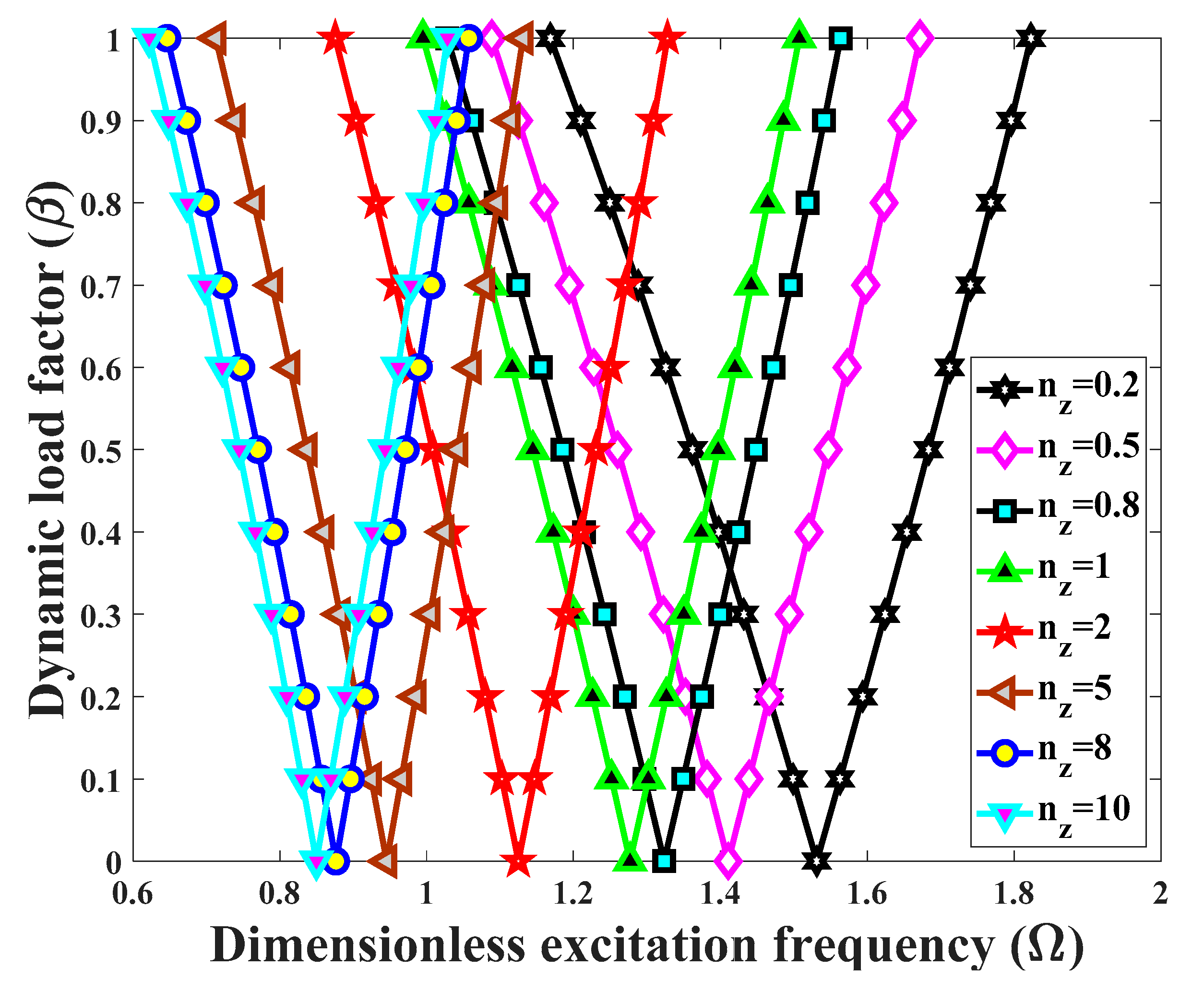
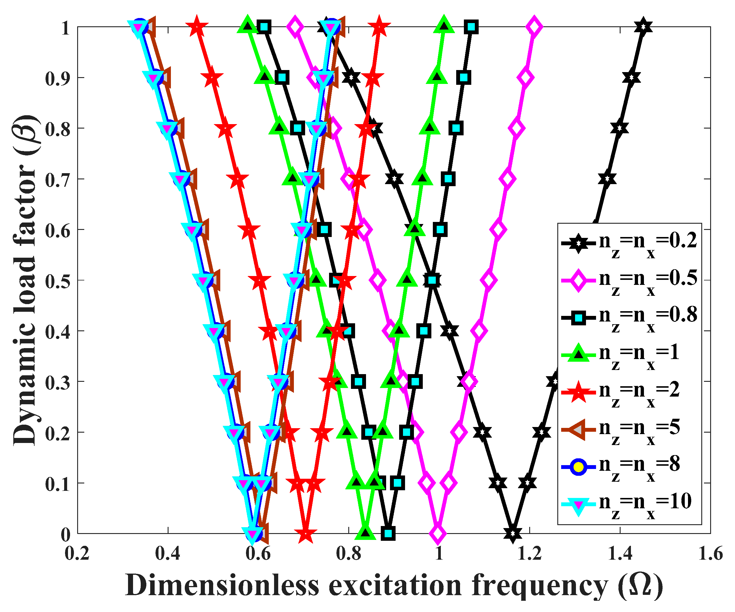
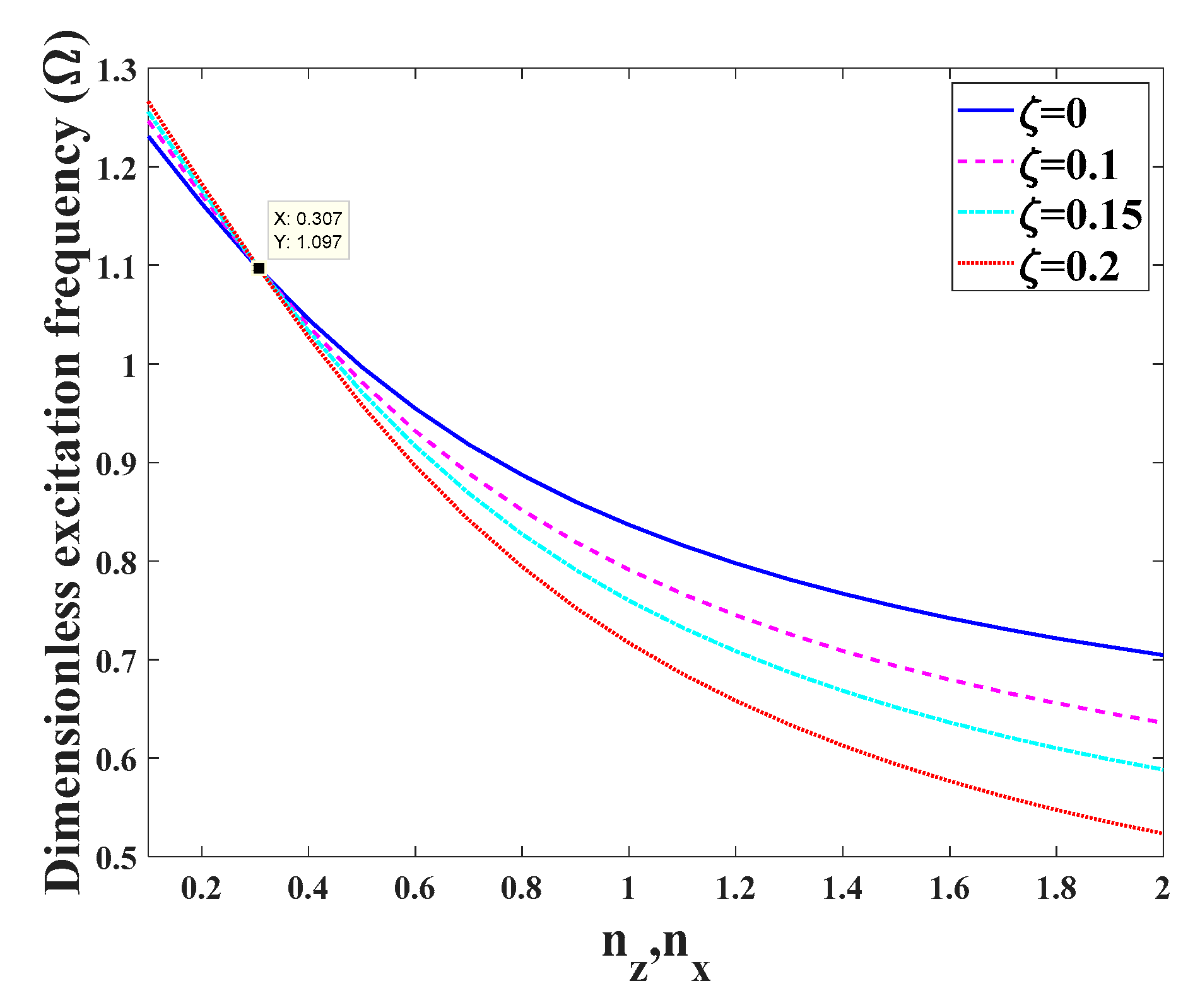
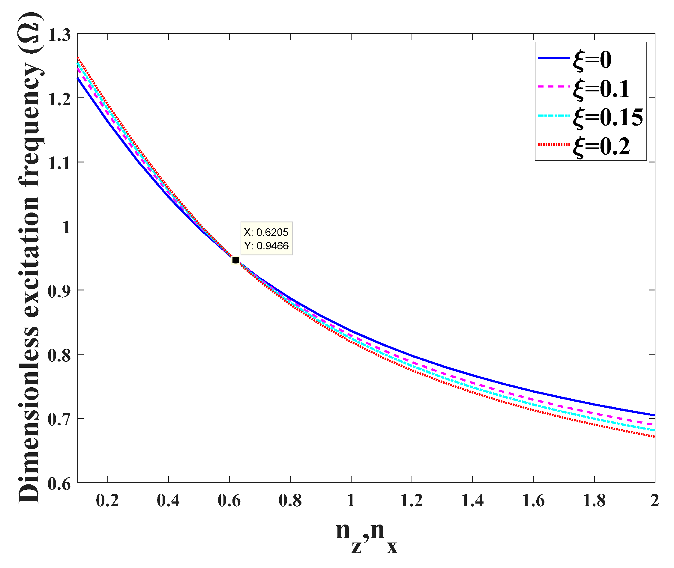
• A simultaneous increase of longitudinal and transverse power indexes yields an overall decrease in the excitation frequencies associated with the DIR origin.
• The control of the dynamic instability for a BD-FG cylindrical shell, is convenient for an appropriate selection of the power indexes.
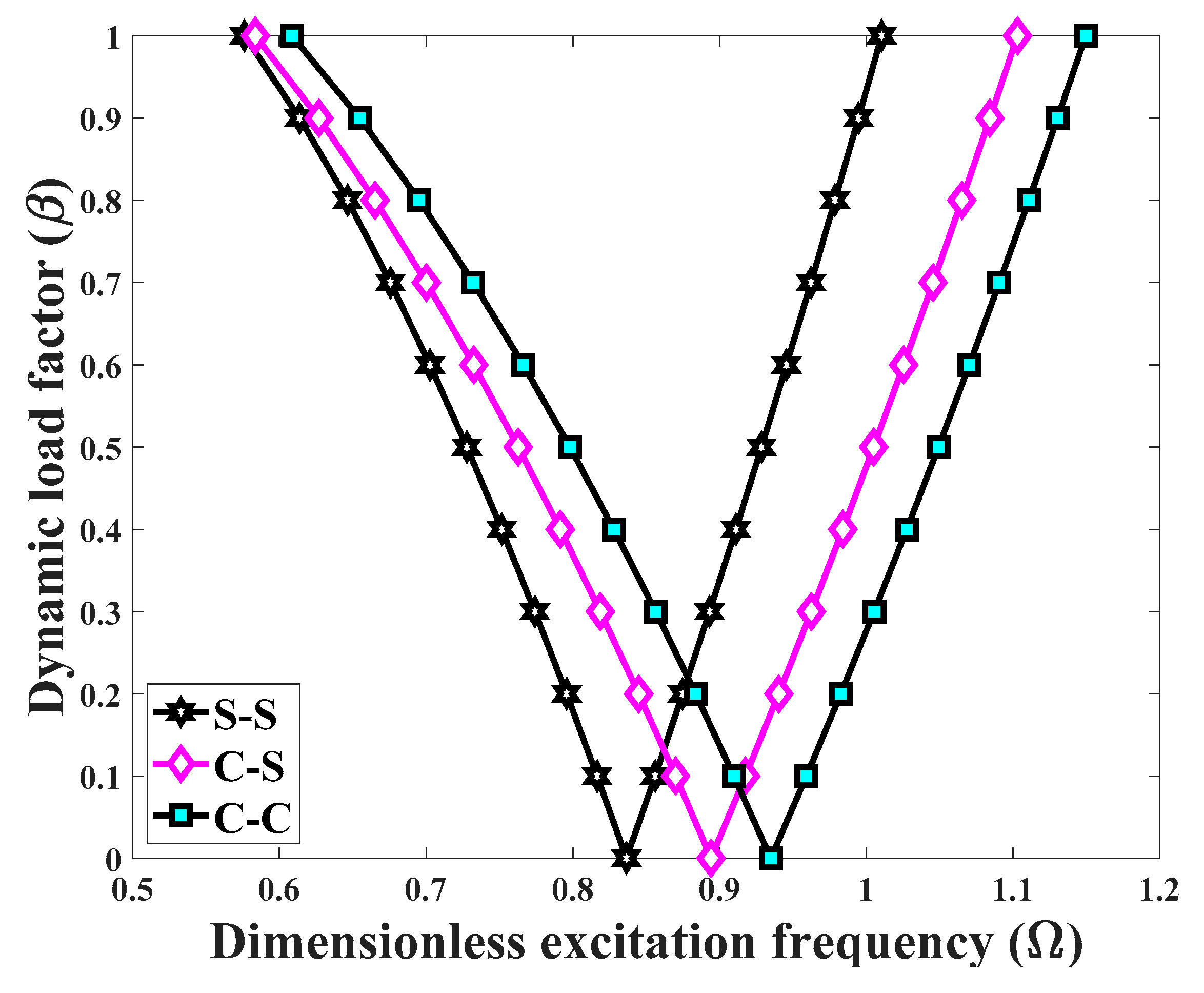
• BD-FG cylindrical shells with a simply support at both ends are more unstable than the clamped-clamped or clamped-simply supported structures, because of their higher deformability.
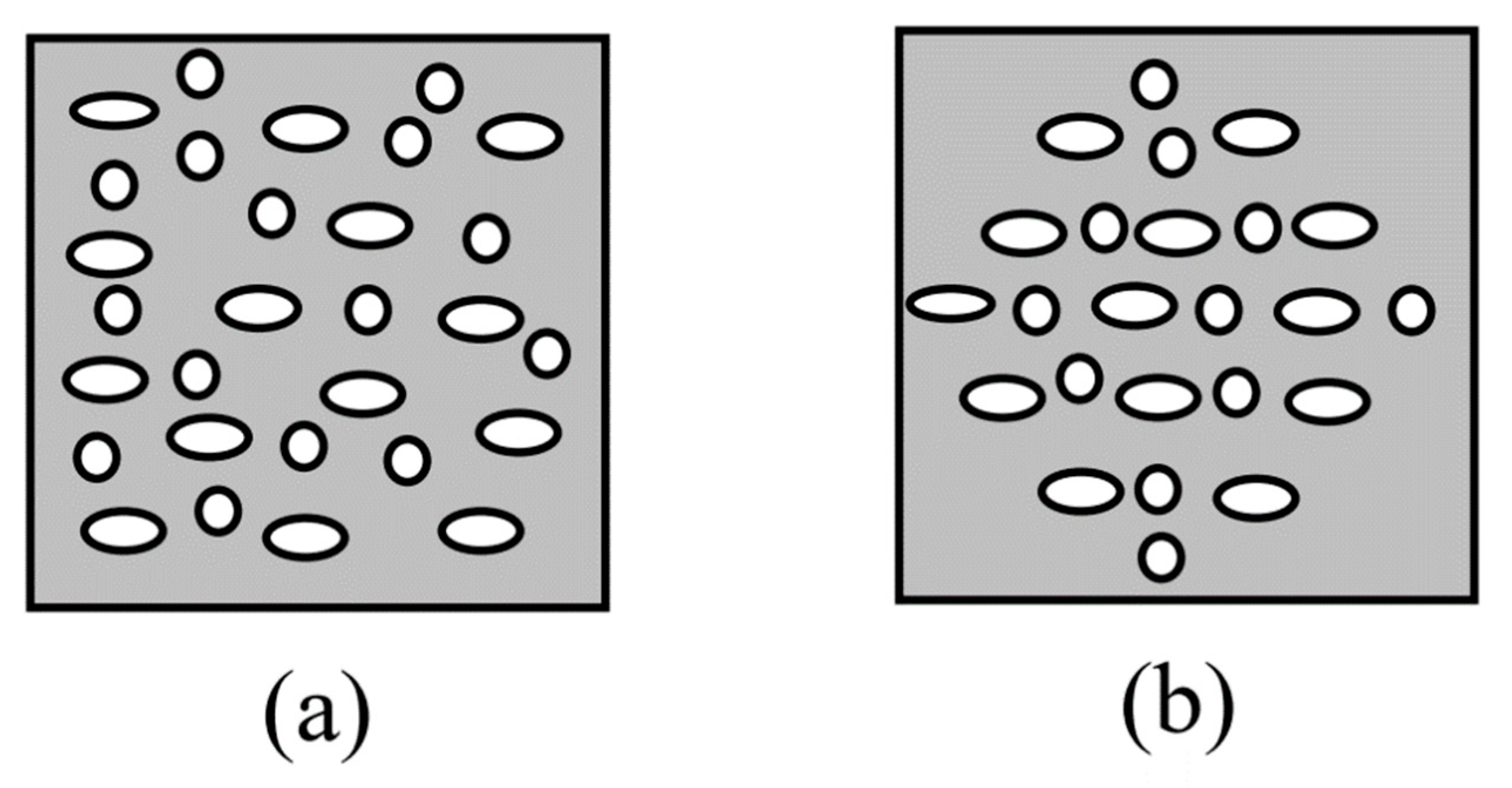
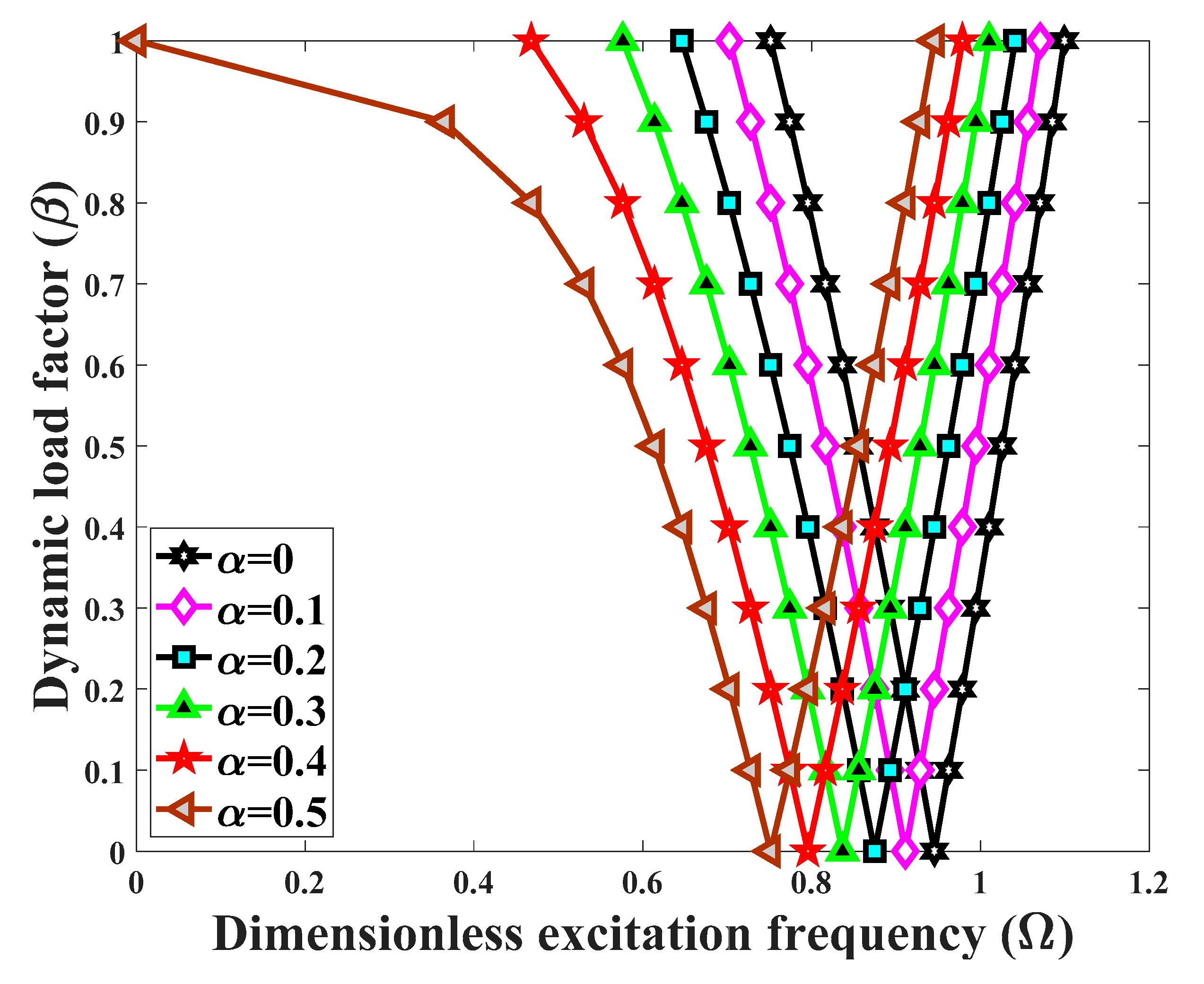
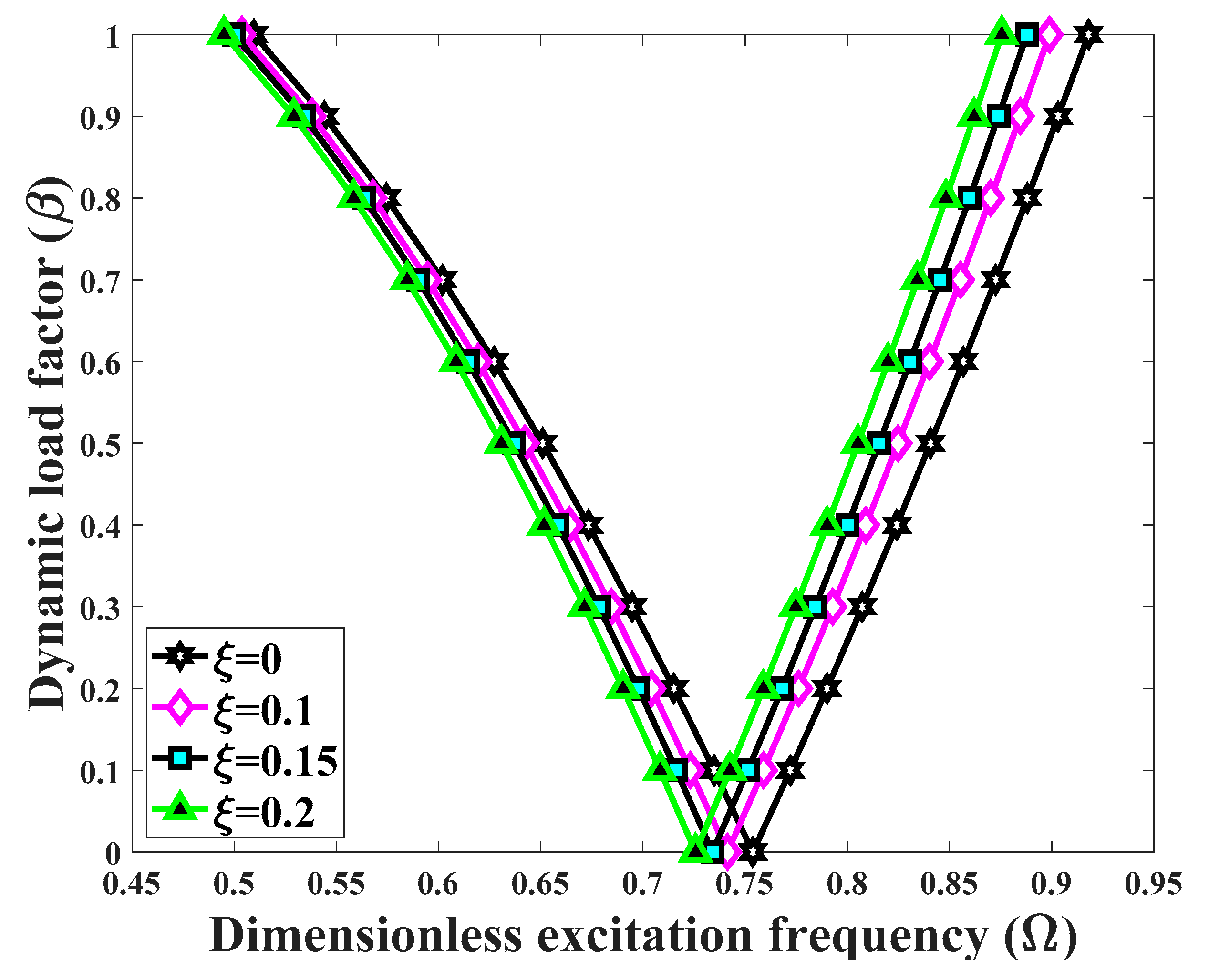
• The effect of coefficients and type of porosity on the structural DIR depend on the extent of the longitudinal and transverse power law indexes. There exists a certain value for these indexes, for which the excitation frequencies corresponding to the DIR can invert their behavior.
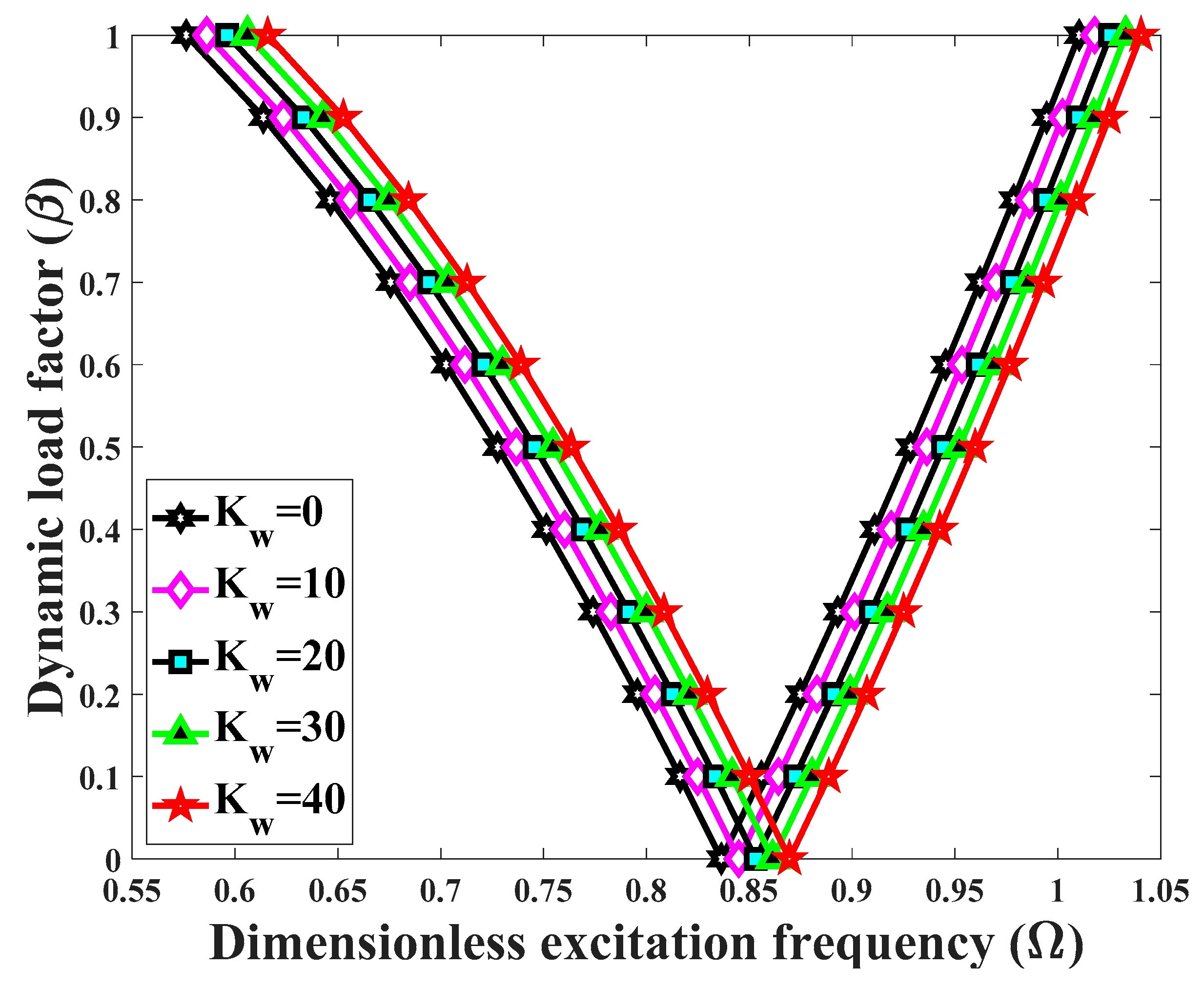
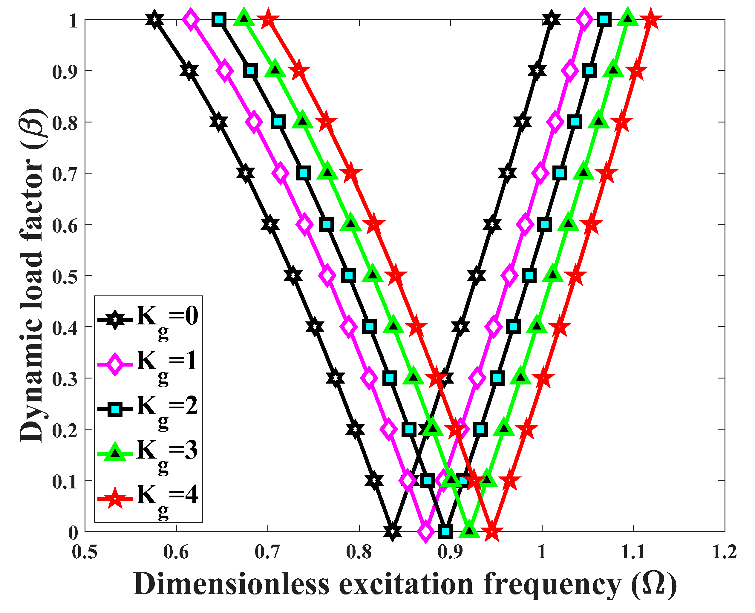
• A general increase in the elastic foundation coefficients yields higher excitation structural frequencies especially when a Pasternak foundation is assumed instead of a Winkler foundation. Anyway, the presence of an elastic foundation makes the structure stiffer and more stable.

References

1. Birman, V.; Byrd, L.W. Modeling and analysis of functionally graded materials and structures. Appl. Mech. Rev. 2007, 60, 195–216. [Google Scholar] [CrossRef]
2. Miyamoto, Y.; Kaysser, W.A.; Rabin, B.H.; Kawasaki, A.; Ford, R.G. Functionally Graded Materials: Design, Processing and Applications; Springer Science & Business Medi: New York, NY, USA, 2013. [Google Scholar]
3. Noda, N. Thermal stresses in functionally graded materials. J. Therm. Stress. 1999, 22, 477–512. [Google Scholar] [CrossRef]
4. Shen, H.S. Functionally Graded Materials: Nonlinear Analysis of Plates and Shells; CRC Press: Boca Raton, FL, USA, 2016. [Google Scholar]
5. Du, C.; Li, Y.; Jin, X. Nonlinear forced vibration of functionally graded cylindrical thin shells. Thin-Walled Struct. 2014, 78, 26–36. [Google Scholar] [CrossRef]
6. Rahimi, G.H.; Ansari, R.; Hemmatnezhad, M. Vibration of functionally graded cylindrical shells with ring support. Sci. Iran. 2011, 18, 1313–1320. [Google Scholar] [CrossRef] [Green Version]
7. Ghasemi, A.R.; Mohandes, M.; Dimitri, R.; Tornabene, F. Agglomeration effects on the vibrations of CNTs/fiber/polymer/metal hybrid laminates cylindrical shell. Compos. Part B Eng. 2019, 167, 700–716. [Google Scholar] [CrossRef]
8. Bich, D.H.; van Dung, D.; Nam, V.H.; Phuong, N.T. Nonlinear static and dynamic buckling analysis of imperfect eccentrically stiffened functionally graded circular cylindrical thin shells under axial compression. Int. J. Mech. Sci. 2013, 74, 190–200. [Google Scholar] [CrossRef]
9. Beni, Y.T.; Mehralian, F.; Zeighampour, H. The modified couple stress functionally graded cylindrical thin shell formulation. Mech. Adv. Mater. Struct. 2016, 23, 791–801. [Google Scholar] [CrossRef]
10. da Silva, F.M.A.; Montes, R.O.P.; Goncalves, P.B.; del Prado, Z.J.G.N. Nonlinear vibrations of fluid-filled functionally graded cylindrical shell considering a time-dependent lateral load and static preload. Proc. Inst. Mech. Eng. Part C J. Mech. Eng. Sci. 2016, 230, 102–119. [Google Scholar] [CrossRef] [Green Version]
11. Bich, D.H.; Nguyen, N.X. Nonlinear vibration of functionally graded circular cylindrical shells based on improved Donnell equations. J. Sound Vib. 2012, 331, 5488–5501. [Google Scholar] [CrossRef]
12. Ghannad, M.; Rahimi, G.H.; Nejad, M.Z. Elastic analysis of pressurized thick cylindrical shells with variable thickness made of functionally graded materials. Compos. Part B Eng. 2013, 45, 388–396. [Google Scholar] [CrossRef]
13. Jafari, A.A.; Khalili, S.M.R.; Tavakolian, M. Nonlinear vibration of functionally graded cylindrical shells embedded with a piezoelectric layer. Thin-Walled Struct. 2014, 79, 8–15. [Google Scholar] [CrossRef]
14. Jin, G.; Xie, X.; Liu, Z. The Haar wavelet method for free vibration analysis of functionally graded cylindrical shells based on the shear deformation theory. Compos. Struct. 2014, 108, 435–448. [Google Scholar] [CrossRef]
15. Liu, Y.Z.; Hao, Y.X.; Zhang, W.; Chen, J.; Li, S.B. Nonlinear dynamics of initially imperfect functionally graded circular cylindrical shell under complex loads. J. Sound Vib. 2015, 348, 294–328. [Google Scholar] [CrossRef]
16. Mehralian, F.; Beni, Y.T. Size-dependent torsional buckling analysis of functionally graded cylindrical shell. Compos. Part B Eng. 2016, 94, 11–25. [Google Scholar] [CrossRef]
17. Sheng, G.G.; Wang, X. Nonlinear response of fluid-conveying functionally graded cylindrical shells subjected to mechanical and thermal loading conditions. Compos. Struct. 2017, 168, 675–684. [Google Scholar] [CrossRef]
18. Sheng, G.G.; Wang, X. The dynamic stability and nonlinear vibration analysis of stiffened functionally graded cylindrical shells. Appl. Math. Model. 2018, 56, 389–403. [Google Scholar] [CrossRef]
19. Zhang, Y.; Huang, H.; Han, Q. Buckling of elastoplastic functionally graded cylindrical shells under combined compression and pressure. Compos. Part B Eng. 2015, 69, 120–126. [Google Scholar] [CrossRef]
20. Sofiyev, A.H.; Hui, D. On the vibration and stability of FGM cylindrical shells under external pressures with mixed boundary conditions by using FOSDT. Thin-Walled Struct. 2019, 134, 419–427. [Google Scholar] [CrossRef]
21. Sun, J.; Xu, X.; Lim, C.W.; Qiao, W. Accurate buckling analysis for shear deformable FGM cylindrical shells under axial compression and thermal loads. Compos. Struct. 2015, 123, 246–256. [Google Scholar] [CrossRef]
22. Huang, H.; Han, Q.; Wei, D. Buckling of FGM cylindrical shells subjected to pure bending load. Compos. Struct. 2011, 93, 2945–2952. [Google Scholar] [CrossRef]
23. Wali, M.; Hentati, T.; Jarraya, A.; Dammak, F. Free vibration analysis of FGM shell structures with a discrete double directors shell element. Compos. Struct. 2015, 125, 295–303. [Google Scholar] [CrossRef]
24. Mohammadi, M.; Arefi, M.; Dimitri, R.; Tornabene, F. Higher-Order Thermo-Elastic Analysis of FG-CNTRC Cylindrical Vessels Surrounded by a Pasternak Foundation. Nanomaterials 2019, 9, 79. [Google Scholar] [CrossRef] [PubMed] [Green Version]
25. Tornabene, F.; Brischetto, S.; Fantuzzi, F.; Viola, E. Numerical and exact models for free vibration analysis of cylindrical and spherical shell panels. Compos. Part B Eng. 2015, 3675, 231–250. [Google Scholar] [CrossRef]
26. Arefi, M.; Mohammadi, M.; Tabatabaeian, A.; Dimitri, R.; Tornabene, F. Two-dimensional thermo-elastic analysis of FG-CNTRC cylindrical pressure vessels. Steel Compos. Struct. 2018, 27, 525–536. [Google Scholar]
27. Nejati, M.; Dimitri, R.; Tornabene, F.; Yas, M.H. Thermal buckling of nanocomposite stiffened cylindrical shells reinforced by functionally Graded wavy Carbon NanoTubes with temperature-dependent properties. Appl. Sci. 2017, 7, 1223. [Google Scholar] [CrossRef] [Green Version]
28. Aragh, B.S.; Hedayati, H. Static response and free vibration of two-dimensional functionally graded metal/ceramic open cylindrical shells under various boundary conditions. Acta Mech. 2012, 223, 309–330. [Google Scholar] [CrossRef]
29. Zafarmand, H.; Hassani, B. Analysis of two-dimensional functionally graded rotating thick disks with variable thickness. Acta Mech. 2014, 225, 453–464. [Google Scholar] [CrossRef]
30. Ebrahimi, M.J.; Najafizadeh, M.M. Free vibration analysis of two-dimensional functionally graded cylindrical shells. Appl. Math. Model. 2014, 38, 308–324. [Google Scholar] [CrossRef]
31. Allahkarami, F.; Satouri, S.; Najafizadeh, M.M. Mechanical buckling of two-dimensional functionally graded cylindrical shells surrounded by Winkler–Pasternak elastic foundation. Mech. Adv. Mater. Struct. 2016, 23, 873–887. [Google Scholar] [CrossRef]
32. Satouri, S.; Kargarnovin, M.H.; Allahkarami, F.; Asanjarani, A. Application of third order shear deformation theory in buckling analysis of 2D-functionally graded cylindrical shell reinforced by axial stiffeners. Compos. Part B Eng. 2015, 79, 236–253. [Google Scholar] [CrossRef]
33. Li, L.; Hu, Y. Torsional vibration of bi-directional functionally graded nanotubes based on nonlocal elasticity theory. Compos. Struct. 2017, 172, 242–250. [Google Scholar] [CrossRef]
34. Kiran, M.C.; Kattimani, S.C. Assessment of porosity influence on vibration and static behaviour of functionally graded magneto-electro-elastic plate: A finite element study. Eur. J. Mech.-A/Solids 2018, 71, 258–277. [Google Scholar] [CrossRef]
35. Kiran, M.C.; Kattimani, S.C.; Vinyas, M. Porosity influence on structural behaviour of skew functionally graded magneto-electro-elastic plate. Compos. Struct. 2018, 191, 36–77. [Google Scholar] [CrossRef]
36. Barati, M.R.; Sadr, M.H.; Zenkour, A.M. Buckling analysis of higher order graded smart piezoelectric plates with porosities resting on elastic foundation. Int. J. Mech. Sci. 2016, 117, 309–320. [Google Scholar] [CrossRef]
37. Wang, Y.Q.; Wan, Y.H.; Zhang, Y.F. Vibrations of longitudinally traveling functionally graded material plates with porosities. Eur. J. Mech.-A/Solids 2017, 66, 55–68. [Google Scholar] [CrossRef]
38. Wang, Y.Q.; Zu, J.W. Vibration behaviors of functionally graded rectangular plates with porosities and moving in thermal environment. Aerosp. Sci. Technol. 2017, 69, 550–562. [Google Scholar] [CrossRef]
39. Wang, Y.; Wu, D. Free vibration of functionally graded porous cylindrical shell using a sinusoidal shear deformation theory. Aerosp. Sci. Technol. 2017, 66, 83–91. [Google Scholar] [CrossRef]
40. Kiani, Y.; Dimitri, R.; Tornabene, F. Free vibration of FG-CNT reinforced composite skew cylindrical shells using the Chebyshev-Ritz formulation. Compos. Part B Eng. 2018, 147, 169–177. [Google Scholar] [CrossRef]
41. Ghadiri, M.; SafarPour, H. Free vibration analysis of size-dependent functionally graded porous cylindrical microshells in thermal environment. J. Therm. Stress. 2017, 40, 55–71. [Google Scholar] [CrossRef]
42. Barati, M.R.; Zenkour, A.M. Vibration analysis of functionally graded graphene platelet reinforced cylindrical shells with different porosity distributions. Mech. Adv. Mater. Struct. 2019, 26, 1580–1588. [Google Scholar] [CrossRef]
43. Malikan, M.; Tornabene, F.; Dimitri, R. Nonlocal three-dimensional theory of elasticity for buckling behavior of functionally graded porous nanoplates using volume integrals. Mater. Res. Express 2018, 5, 095006. [Google Scholar] [CrossRef]
44. Malikan, M.; Tornabene, F.; Dimitri, R. Effect of sinusoidal corrugated geometries on the vibrational response of viscoelastic nanoplates. Appl. Sci. 2018, 8, 1432. [Google Scholar] [CrossRef] [Green Version]
45. Arefi, M.; Bidgoli, E.M.R.; Dimitri, R.; Tornabene, F. Free vibrations of functionally graded polymer composite nanoplates reinforced with graphene nanoplatelets. Aerosp. Sci. Technol. 2018, 81, 108–117. [Google Scholar] [CrossRef]
46. Jouneghani, F.Z.; Dimitri, R.; Tornabene, F. Structural response of porous FG nanobeams under hygro-thermo-mechanical loadings. Compos. Part B Eng. 2018, 152, 71–78. [Google Scholar] [CrossRef]
47. Arefi, M.; Bidgoli, E.M.R.; Dimitri, R.; Bacciocchi, M.; Tornabene, F. Nonlocal bending analysis of curved nanobeams reinforced by graphene nanoplatelets. Compos. Part B Eng. 2019, 166, 1–12. [Google Scholar] [CrossRef]
48. Bagherizadeh, E.; Kiani, Y.; Eslami, M.R. Mechanical buckling of functionally graded material cylindrical shells surrounded by Pasternak elastic foundation. Compos. Struct. 2011, 93, 3063–3071. [Google Scholar] [CrossRef]
49. Shu, C. Differential Quadrature and Its Application in Engineering; Springer Science & Business Media: New York, NY, USA, 2012. [Google Scholar]
50. Tornabene, F.; Fantuzzi, N.; Ubertini, F.; Viola, E. Strong formulation finite element method based on differential quadrature: A survey. Appl. Mech. Rev. 2015, 67, 1–55. [Google Scholar] [CrossRef]
51. Tornabene, F.; Fantuzzi, N.; Bacciocchi, M.; Dimitri, R. Free vibrations of composite oval and elliptic cylinders by the generalized differential quadrature method. Thin-Walled Struct. 2015, 97, 114–129. [Google Scholar] [CrossRef]
52. Yas, M.; Nejati, M.; Asanjarani, A. Free vibration analysis of continuously graded fiber reinforced truncated conical shell via third-order shear deformation theory. J. Solid Mech. 2016, 8, 212–231. [Google Scholar]
53. Kamarian, S.; Salim, M.; Dimitri, R.; Tornabene, F. Free vibration analysis conical shells reinforced with agglomerated Carbon Nanotubes. Int. J. Mech. Sci. 2016, 108–109, 157–165. [Google Scholar] [CrossRef]
54. Liu, G.R.; Wu, T.Y. In-plane vibration analyses of circular arches by the generalized differential quadrature rule. Int. J. Mech. Sci. 2001, 43, 2597–2611. [Google Scholar] [CrossRef]
55. Tornabene, F.; Dimitri, R. A numerical study of the seismic response of arched and vaulted structures made of isotropic or composite materials. Eng. Struct. 2018, 159, 332–366. [Google Scholar] [CrossRef]
56. Dimitri, R.; Tornabene, F.; Zavarise, G. Analytical and numerical modeling of the mixed-mode delamination process for composite moment-loaded double cantilever beams. Compos. Struct. 2018, 187, 535–553. [Google Scholar] [CrossRef]
57. Dimitri, R.; Tornabene, F. Numerical Study of the Mixed-Mode Delamination of Composite Specimens. J. Compos. Sci. 2018, 2, 30. [Google Scholar] [CrossRef] [Green Version]
58. Tomasiello, S. Differential quadrature method: Application to initial-boundary-value problems. J. Sound Vib. 1998, 218, 573–585. [Google Scholar] [CrossRef]
59. Tornabene, F.; Dimitri, R.; Viola, E. Transient dynamic response of generally-shaped arches based on a GDQ-time-stepping method. Int. J. Mech. Sci. 2016, 114, 277–314. [Google Scholar] [CrossRef]
60. Bolotin, V.V. The dynamic stability of elastic systems. Am. J. Phys. 1965, 33, 752–753. [Google Scholar] [CrossRef]
61. Khazaeinejad, P.; Najafizadeh, M.M. Mechanical buckling of cylindrical shells with varying material properties. Proc. Inst. Mech. Eng. Part C J. Mech. Eng. Sci. 2010, 224, 1551–1557. [Google Scholar] [CrossRef]
Figure 1. Geometrical scheme of a bi-directional (BD)-functionally graded (FG) porous cylindrical shell embedded in an elastic foundation.
Applsci 10 01345 g001
Figure 2. Distribution of porosity: (a) even porosity, (b) uneven porosity.
Applsci 10 01345 g002
Figure 3. Effect of the thickness-to-radius ratio on the dynamic instability region (DIR) for a BD-FG cylindrical shell with R = 0.5   m , L / R = 1 , n x = n z = 1 , α = 0.3 .
Applsci 10 01345 g003
Figure 4. Effect of the length-to-radius ratio on the DIR for a BD-FG cylindrical shell with R = 0.5   m , h / R = 0.02 , n x = n z = 1 , α = 0.3 .
Applsci 10 01345 g004
Figure 5. Effect of the static load factor on the DIR for a BD-FG cylindrical shell with R = 0.5   m , h / R = 0.02 , L / R = 1 , n x = n z = 1 , α = 0.3 .
Applsci 10 01345 g005
Figure 6. Effect of boundary conditions on the DIR for a BD-FG cylindrical shell with R = 0.5   m , h / R = 0.02 , L / R = 1 , n x = n z = 1 , α = 0.3 .
Applsci 10 01345 g006
Figure 7. Effect of the longitudinal power index on the DIR for a FG cylindrical shell with R = 0.5   m , h / R = 0.02 , L / R = 1 , n z = 0 , α = 0.3 .
Applsci 10 01345 g007
Figure 8. Effect of the transverse power index on the DIR for a BD-FG cylindrical shell with R = 0.5   m , h / R = 0.02 , L / R = 1 , n x = 0 , α = 0.3 .
Applsci 10 01345 g008
Figure 9. Effect of the longitudinal and transverse power indexes on the DIR for a FG cylindrical shell with R = 0.5   m , h / R = 0.02 , L / R = 1 , α = 0.3 .
Applsci 10 01345 g009
Figure 10. Effect of the even porosity volume fraction ζ on the dimensionless excitation frequency versus the longitudinal and transverse power indexes for a BD-FG porous cylindrical shell with R = 0.5   m , h / R = 0.02 , L / R = 1 , α = 0.3 , β = 0 .
Applsci 10 01345 g010
Figure 11. Effect of the even porosity volume fraction ζ on the DIR for a BD-FG porous cylindrical shell with R = 0.5   m , h / R = 0.02 , L / R = 1 , α = 0.3 , n x = n z = 0.15 .
Applsci 10 01345 g011
Figure 12. Effect of the even porosity volume fraction ζ on the DIR for a BD-FG porous cylindrical shell with R = 0.5   m , h / R = 0.02 , L / R = 1 , α = 0.3 , n x = n z = 0.15 .
Applsci 10 01345 g012
Figure 13. Effect of the uneven porosity volume fraction ξ on the dimensionless excitation frequency versus the longitudinal and transverse power indexes for a BD-FG porous cylindrical shell with R = 0.5   m , h / R = 0.02 , L / R = 1 , α = 0.3 , β = 0 .
Applsci 10 01345 g013
Figure 14. Effect of the uneven porosity volume fraction ξ on the DIR for a BD-FG porous cylindrical shell with R = 0.5   m , h / R = 0.02 , L / R = 1 , α = 0.3 , n x = n z = 0.15 .
Applsci 10 01345 g014
Figure 15. Effect of the uneven porosity volume fraction ξ on the DIR for a BD-FG porous cylindrical shell with R = 0.5   m , h / R = 0.02 , L / R = 1 , α = 0.3 , n x = n z = 0.15 .
Applsci 10 01345 g015
Figure 16. Effect of the Winkler coefficient on the DIR for a BD-FG cylindrical shell with R = 0.5   m , h / R = 0.02 , L / R = 1 , α = 0.3 , K g = 0 , n x = n z = 1.5 .
Applsci 10 01345 g016
Figure 17. Effect of the Pasternak coefficient on the DIR for a BD-FG cylindrical shell with R = 0.5   m , h / R = 0.02 , L / R = 1 , α = 0.3 , K w = 0 , n x = n z = 1 .
Applsci 10 01345 g017