A Numerical Model for Simulating Ground Motions for the Korean Peninsula


Abstract
Featured Application
Abstract
1. Introduction
2. Ground Motions Collected for Developing the Ground Motion Simulation Model
3. Ground Motion Simulation Model
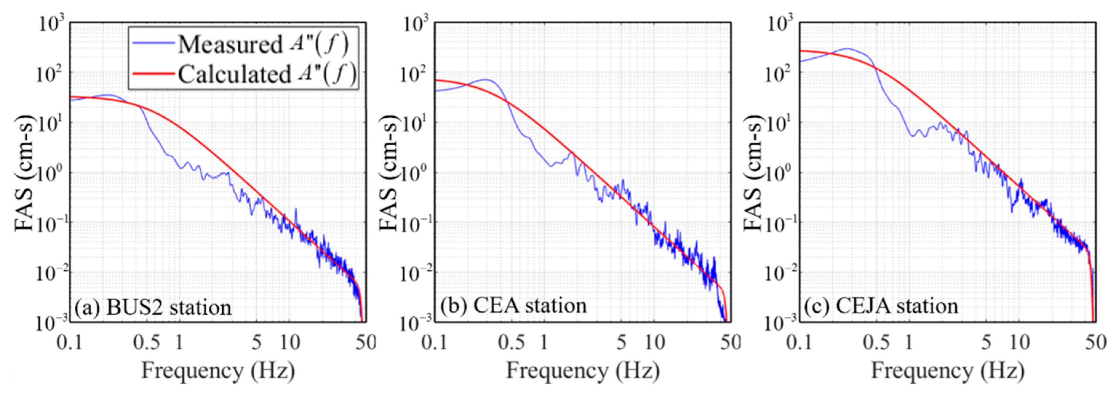
3.1. Stochastic Point-Source Model Estimation
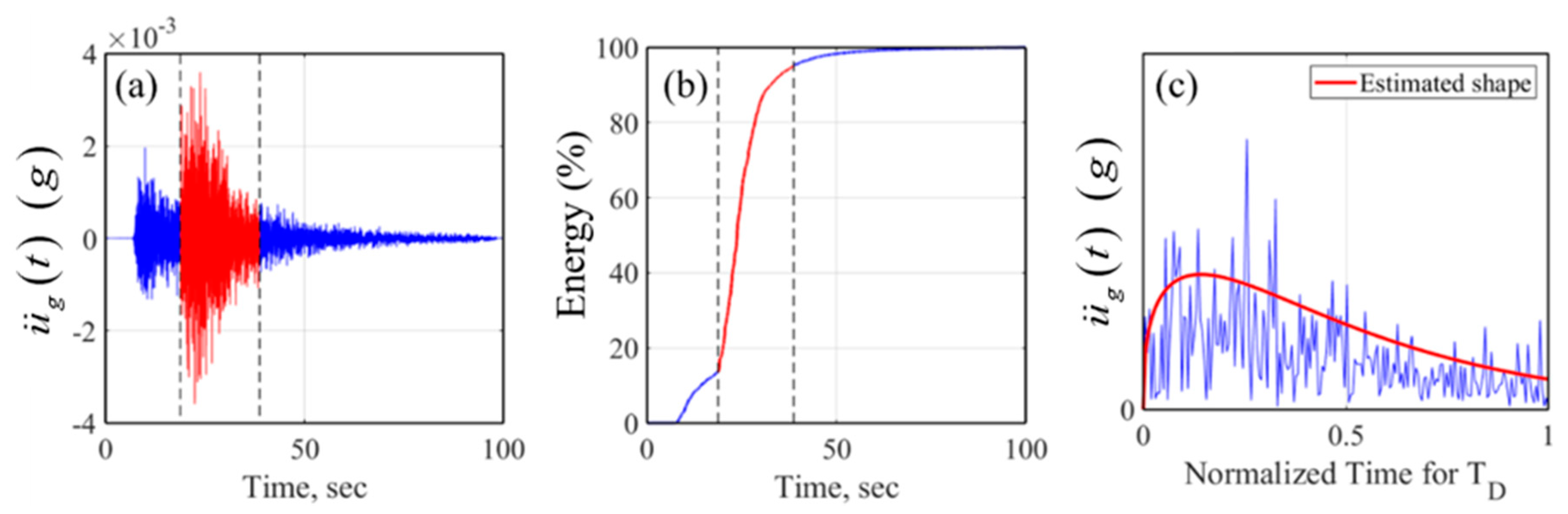
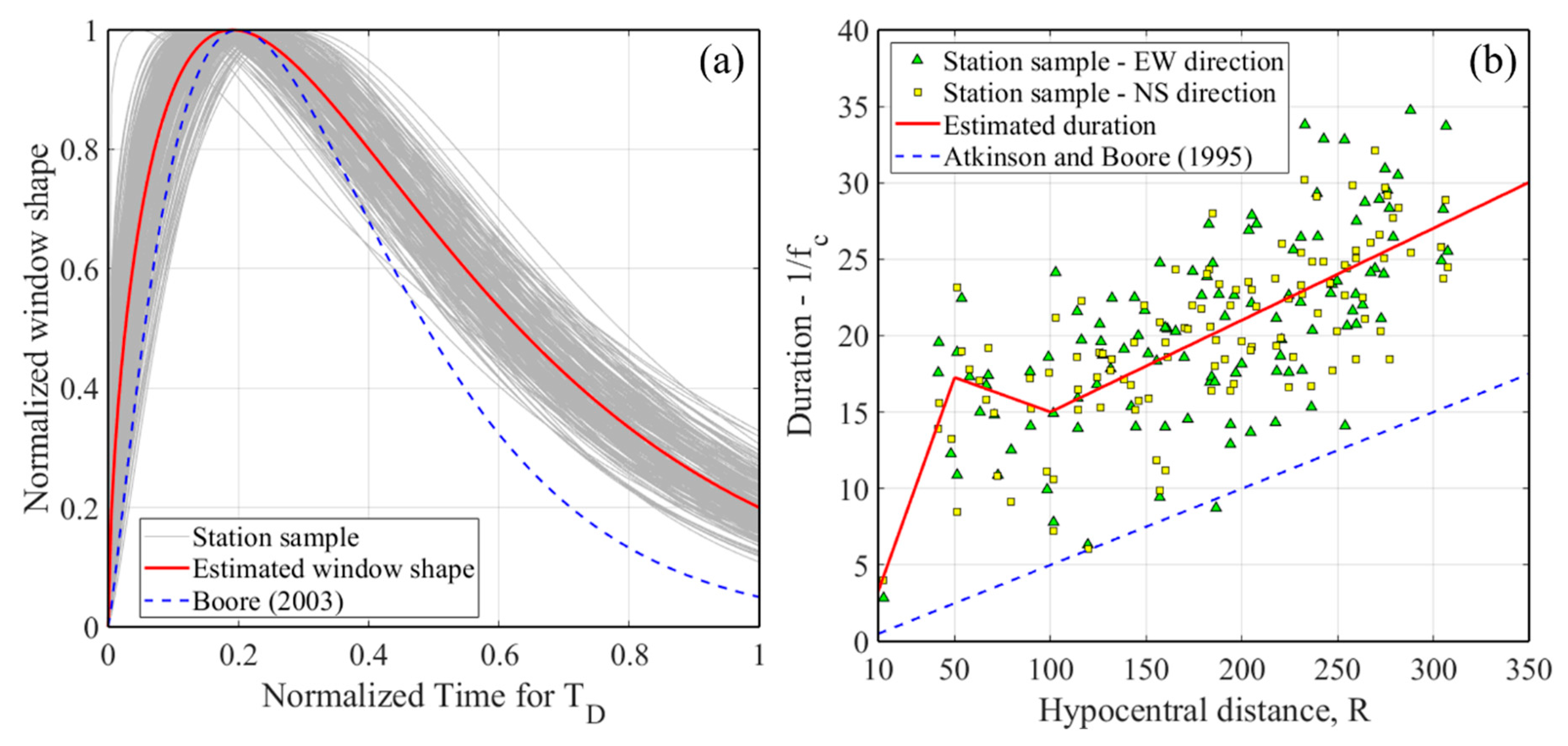
3.2. Shaping Window Model Estimation
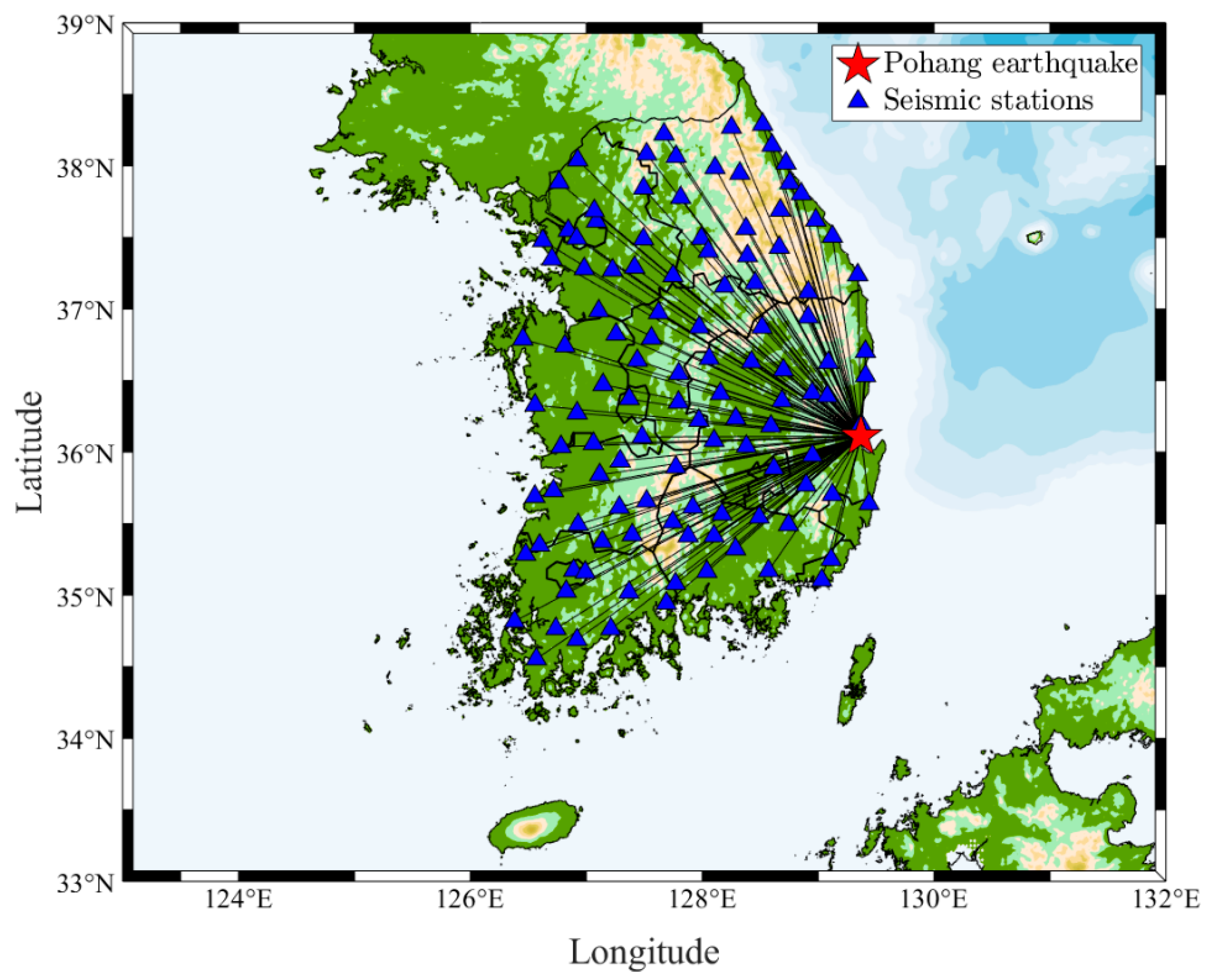
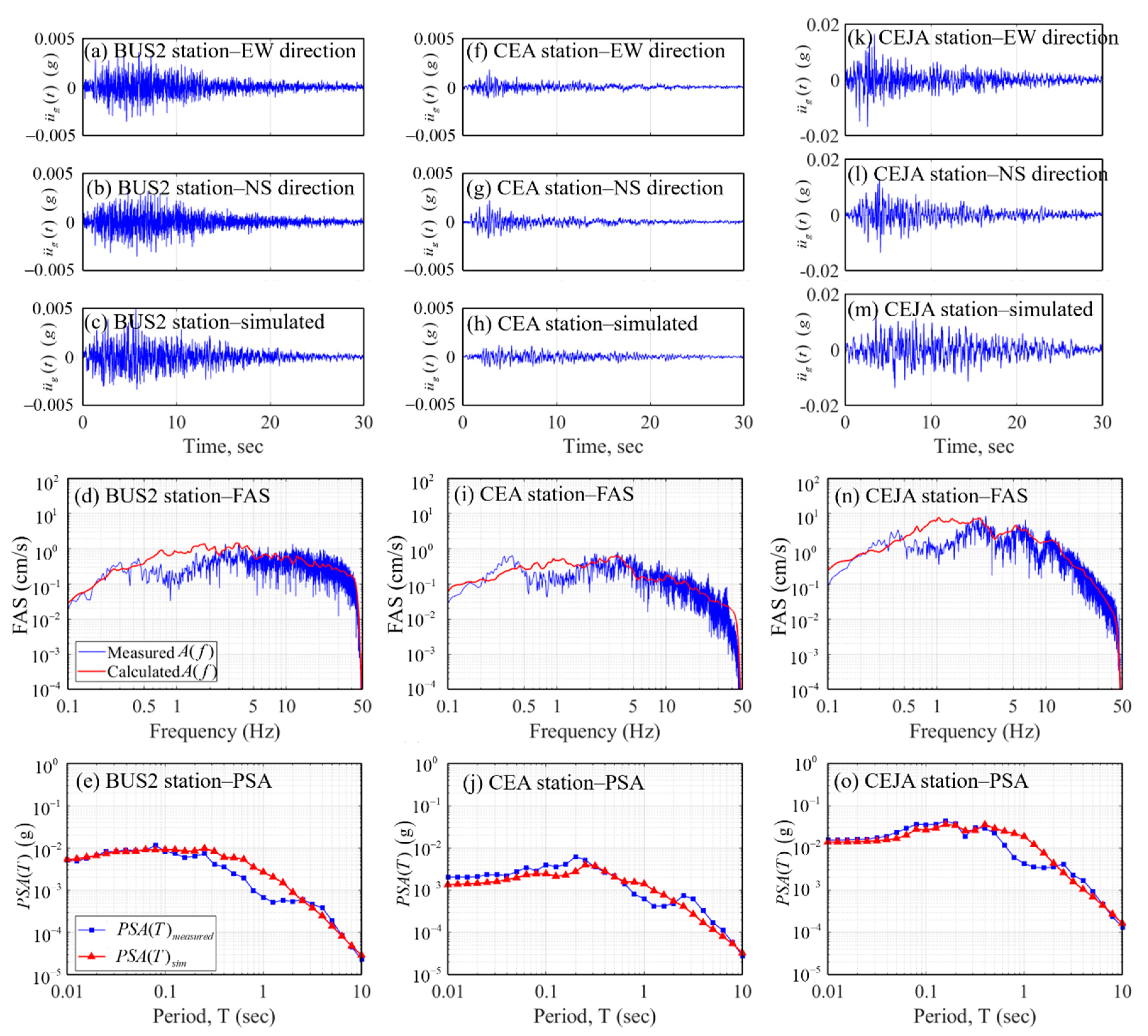
4. Ground Motion Simulation for the 2017 Pohang Earthquake
- (1)
- White noise is first generated in time domain for a duration time of the ground motion (Equation (12)).
- (2)
- The noise is then windowed using the shaping window model (Equation (10)).
- (3)
- The windowed noise is transformed into the frequency domain.
- (4)
- The of the noise is normalized by the square-root of the mean square of in all frequencies.
- (5)
- The normalized is then multiplied by the stochastic simulation model (Equation (2)).
- (6)
- The resulting is transformed back to the time domain, which is a simulated ground motion.
5. Conclusions
- (1)
- Source, path, and site effect functions were developed for the stochastic point-source model, which reflected the seismological characteristics of the Korean Peninsula.
- (2)
- To generate ground motions in the time domain that represents ground motions recorded in the Korean Peninsula, an envelope shape and a duration time function were proposed based on the ground motions recorded at 111 stations.
- (3)
- In order to verify the accuracy of the proposed numerical model, residuals measuring the difference in between recorded and simulated ground motions were calculated for 111 stations. It was observed that ground motions in the Korean Peninsula were simulated accurately using the proposed numerical model, which included proper source, path, and site effect functions.
- (4)
- The results of this study reveal the potential of the proposed numerical model to simulate input ground motions for low-to-moderate seismic regions, such as the Korean Peninsula.
Author Contributions
Funding
Acknowledgments
Conflicts of Interest
Appendix A

| No. | Station | No. | Station | No. | Station | No. | Station | ||||
|---|---|---|---|---|---|---|---|---|---|---|---|
| 1 | ADO2 | 0.0092 | 29 | GOCB | 0.0203 | 57 | JEU2 | −0.0035 | 85 | SCHA | 0.0161 |
| 2 | ADOA | 0.0284 | 30 | GSG | −0.0112 | 58 | JINA | 0.0197 | 86 | SEHB | 0.0259 |
| 3 | BON | 0.0182 | 31 | GUM | 0.0447 | 59 | JMJ | 0.0149 | 87 | SEO2 | 0.0059 |
| 4 | BOSB | 0.0150 | 32 | GUS | 0.0017 | 60 | JNPA | 0.0221 | 88 | SES2 | 0.0132 |
| 5 | BSA | 0.0208 | 33 | GUWB | 0.0235 | 61 | JUR | 0.0120 | 89 | SHHB | 0.0149 |
| 6 | BURB | 0.0254 | 34 | GWJ | 0.0289 | 62 | KAWA | 0.0227 | 90 | SKC2 | 0.0102 |
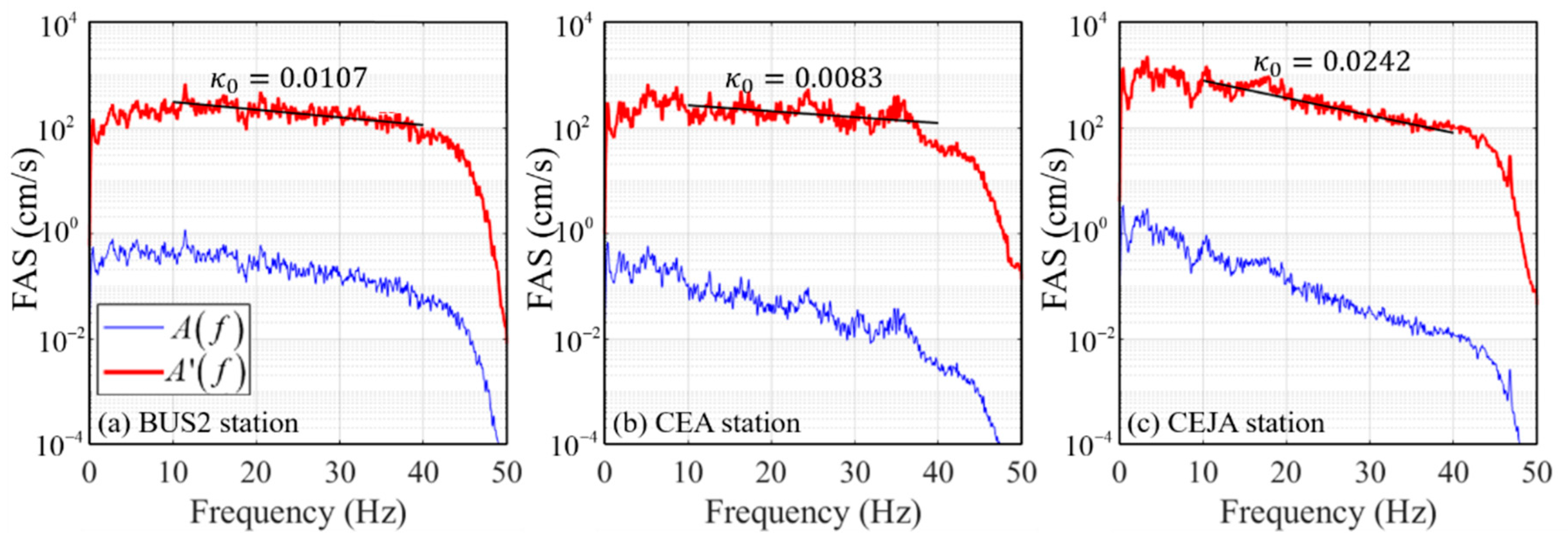
| 7 | BUS | 0.0107 | 35 | GWYB | 0.0142 | 63 | KCH2 | 0.0312 | 91 | SMKB | 0.0267 |
| 8 | BUYB | 0.0093 | 36 | HAC | 0.0226 | 64 | KMSA | 0.0234 | 92 | SUCA | 0.0149 |
| 9 | CEA | 0.0083 | 37 | HAD | 0.0352 | 65 | KOJ2 | 0.0241 | 93 | SWO | 0.0255 |
| 10 | CEJA | 0.0242 | 38 | HALB | 0.0253 | 66 | KWJ2 | 0.0112 | 94 | TBA2 | 0.0352 |
| 11 | CHC2 | 0.0161 | 39 | HANB | 0.0150 | 67 | MAS2 | 0.0087 | 95 | TEJ2 | 0.0370 |
| 12 | CHJ2 | 0.0111 | 40 | HCNA | 0.0245 | 68 | MGY2 | 0.0177 | 96 | TOHA | 0.0183 |
| 13 | CHO | 0.0253 | 41 | HES | 0.0167 | 69 | MIYA | 0.0287 | 97 | ULJ2 | 0.0118 |
| 14 | CHR | 0.0254 | 42 | HWCA | 0.0192 | 70 | MOP | 0.0218 | 98 | USN2 | 0.0275 |
| 15 | CHYB | 0.0219 | 43 | HWCB | 0.0251 | 71 | MUS2 | 0.0261 | 99 | WJU2 | 0.0472 |
| 16 | CIGB | 0.0160 | 44 | ICN | 0.0131 | 72 | NAJ | 0.0186 | 100 | YAPA | 0.0208 |
| 17 | CPR2 | 0.0077 | 45 | IJA2 | 0.0197 | 73 | NAWB | 0.0122 | 101 | YAY | 0.0227 |
| 18 | CSO | 0.0277 | 46 | IJAA | 0.0235 | 74 | NOW | −0.0065 | 102 | YAYA | 0.0242 |
| 19 | CWO2 | 0.0096 | 47 | IKSA | 0.0140 | 75 | OKCB | 0.0109 | 103 | YCH | 0.0179 |
| 20 | DAG2 | 0.0197 | 48 | IMSA | 0.0235 | 76 | OKEB | 0.0269 | 104 | YEG | 0.0051 |
| 21 | DAU | 0.0061 | 49 | IMWB | 0.0205 | 77 | PHA2 | 0.0130 | 105 | YEYB | 0.0190 |
| 22 | DGY2 | 0.0055 | 50 | INCA | 0.0125 | 78 | PORA | 0.0216 | 106 | YINB | 0.0344 |
| 23 | DUSB | 0.0121 | 51 | JAHA | 0.0288 | 79 | PTK | 0.0113 | 107 | YNCB | 0.0214 |
| 24 | EMSB | 0.0279 | 52 | JASA | 0.0162 | 80 | PUAA | 0.0182 | 108 | YOA | 0.0140 |
| 25 | EURB | 0.0130 | 53 | JECB | 0.0122 | 81 | PYC | 0.0237 | 109 | YOCB | 0.0058 |
| 26 | EUSB | 0.0212 | 54 | JEJB | 0.0162 | 82 | PYCA | 0.0199 | 110 | YODB | 0.0222 |
| 27 | GAPB | 0.0288 | 55 | JEO2 | 0.0021 | 83 | SACA | 0.0155 | 111 | YOJB | 0.0170 |
| 28 | GIC | 0.0110 | 56 | JES | 0.0340 | 84 | SAJ | 0.0227 | Median | 0.0192 | |
| No. | , Hz | , Dyne-cm | No. | , Hz | , Dyne-cm | No. | , Hz | , Dyne-cm | No. | , Hz | , Dyne-cm |
|---|---|---|---|---|---|---|---|---|---|---|---|
| 1 | 0.59 | 29 | 0.70 | 57 | 0.44 | 85 | 0.76 | ||||
| 2 | 0.46 | 30 | 0.22 | 58 | 0.50 | 86 | 0.48 | ||||
| 3 | 0.84 | 31 | 1.42 | 59 | 0.36 | 87 | 0.25 | ||||
| 4 | 0.55 | 32 | 0.66 | 60 | 0.64 | 88 | 0.63 | ||||
| 5 | 1.05 | 33 | 0.49 | 61 | 0.63 | 89 | 0.39 | ||||
| 6 | 0.43 | 34 | 1.46 | 62 | 0.55 | 90 | 0.35 | ||||
| 7 | 0.56 | 35 | 0.58 | 63 | 1.37 | 91 | 1.17 | ||||
| 8 | 0.56 | 36 | 0.44 | 64 | 0.63 | 92 | 0.53 | ||||
| 9 | 0.32 | 37 | 1.43 | 65 | 0.74 | 93 | 0.89 | ||||
| 10 | 0.43 | 38 | 0.72 | 66 | 0.78 | 94 | 1.46 | ||||
| 11 | 0.48 | 39 | 0.49 | 67 | 1.21 | 95 | 1.29 | ||||
| 12 | 0.50 | 40 | 0.80 | 68 | 0.36 | 96 | 0.59 | ||||
| 13 | 1.05 | 41 | 0.84 | 69 | 0.80 | 97 | 0.28 | ||||
| 14 | 1.46 | 42 | 0.58 | 70 | 0.94 | 98 | 0.97 | ||||
| 15 | 0.32 | 43 | 0.68 | 71 | 1.31 | 99 | 1.37 | ||||
| 16 | 0.44 | 44 | 0.45 | 72 | 1.23 | 100 | 0.48 | ||||
| 17 | 0.58 | 45 | 0.66 | 73 | 0.35 | 101 | 0.87 | ||||
| 18 | 0.74 | 46 | 0.43 | 74 | 0.32 | 102 | 0.44 | ||||
| 19 | 0.43 | 47 | 0.46 | 75 | 0.40 | 103 | 0.80 | ||||
| 20 | 0.78 | 48 | 0.66 | 76 | 0.56 | 104 | 1.34 | ||||
| 21 | 0.63 | 49 | 0.50 | 77 | 0.50 | 105 | 0.30 | ||||
| 22 | 0.23 | 50 | 0.32 | 78 | 0.63 | 106 | 0.48 | ||||
| 23 | 0.53 | 51 | 0.92 | 79 | 0.52 | 107 | 0.50 | ||||
| 24 | 0.84 | 52 | 0.61 | 80 | 0.78 | 108 | 1.14 | ||||
| 25 | 0.61 | 53 | 0.40 | 81 | 1.27 | 109 | 0.25 | ||||
| 26 | 0.45 | 54 | 0.17 | 82 | 0.61 | 110 | 0.28 | ||||
| 27 | 0.52 | 55 | 0.43 | 83 | 0.48 | 111 | 0.39 | ||||
| 28 | 1.17 | 56 | 1.14 | 84 | 1.05 | Median | 0.58 |
References
- Johnston, A.C. Seismic Moment Assessment of Earthquakes in Stable Continental Regions-I. Instrumental Seismicity. Geophys. J. Int. 1996, 124, 381–414. [Google Scholar] [CrossRef]
- Schulte, S.M.; Mooney, W.D. An Updated Global Earthquake Catalogue for Stable Continental Regions: Reassessing the Correlation with Ancient Rifts. Geophys. J. Int. 2005, 161, 707–721. [Google Scholar] [CrossRef]
- Lee, K.; Yang, W.S. Historical Seismicity of Korea. Bull. Seismol. Soc. Am. 2006, 96, 846–855. [Google Scholar] [CrossRef]
- Wen, Y.K.; Collins, K.R.; Han, S.W.; Elwood, K.J. Dual-level designs of buildings under seismic loads. Struct. Saf. 1996, 18, 195–224. [Google Scholar] [CrossRef]
- Lee, L.H.; Lee, H.H.; Han, S.W. Method of selecting design earthquake ground motions for tall buildings. Struct. Des. Tall. Spec. 2000, 9, 201–213. [Google Scholar] [CrossRef]
- Han, S.W.; Seok, S.W. Efficient Procedure for Selecting and Scaling Ground Motions for Response History Analysis. J. Struct. Eng. 2014, 140, 06013004. [Google Scholar] [CrossRef]
- Saragoni, G.; Hart, G. Simulation of Artificial Earthquakes. Earthq. Eng. Struct. Dyn. 1974, 2, 249–267. [Google Scholar] [CrossRef]
- Hanks, T.C.; McGuire, R.K. The Character of High-frequency Strong Ground Motion. Bull. Seismol. Soc. Am. 1981, 71, 2071–2095. [Google Scholar]
- Boore, D.M. Stochastic Simulation of High-frequency Ground Motions Based on Seismological Models of the Radiated Spectra. Bull. Seismol. Soc. Am. 1983, 73, 1865–1894. [Google Scholar]
- Boore, D.M.; Atkinson, G.M. Stochastic Prediction of Ground Motion and Spectral Response Parameters at Hard-rock Sites in Eastern North America. Bull. Seismol. Soc. Am. 1987, 77, 440–467. [Google Scholar]
- Atkinson, G.M.; Boore, D.M. Ground-motion Relations for Eastern North America. Bull. Seismol. Soc. Am. 1995, 85, 17–30. [Google Scholar]
- Boore, D.M. Simulation of Ground Motion Using the Stochastic Method. Pure. Appl. Geophys. 2003, 160, 635–676. [Google Scholar] [CrossRef]
- Papazafeiropoulos, G.; Plevris, V. OpenSeismoMatlab: A New Open-source Software for Strong Ground Motion Data Processing. Heliyon 2018, 4, e00784. [Google Scholar] [CrossRef] [PubMed]
- Nakamura, Y. A Method for Dynamic Characteristics Estimation of Subsurface Using Microtremor on the Ground Surface. Q. Rep. Railw. Tech. Res. Inst. 1989, 30, 25–33. [Google Scholar]
- Atkinson, G.M.; Cassidy, J.F. Integrated Use of Seismograph and Strong-Motion Data to Determine Soil Amplification: Response of the Fraser River Delta to the Duvall and Georgia Strait Earthquakes. Bull. Seismol. Soc. Am. 2000, 90, 1028–1040. [Google Scholar] [CrossRef]
- Zhao, J.X.; Irikura, K.; Zhang, J.; Yoshimitsu, F.; Somerville, P.G.; Asano, A.; Ohno, Y.; Oouchi, T.; Takahashi, T.; Ogawa, H. An Empirical Site-Classification Method for Strong-Motion Stations in Japan Using H/V Response Spectral Ratio. Bull. Seismol. Soc. Am. 2006, 96, 914–925. [Google Scholar] [CrossRef]
- Zandieh, A.; Pezeshk, S. Investigation of Geometrical Spreading and Quality Factor Functions in the New Madrid Seismic Zone. Bull. Seismol. Soc. Am. 2010, 100, 2185–2195. [Google Scholar] [CrossRef]
- Brune, J. Tectonic Stress and the Spectra of Seismic Shear Waves. J. Geophys. Res. 1970, 75, 4997–5009. [Google Scholar] [CrossRef]
- Brune, J. Correction: Tectonic Stress and the Spectra of Seismic Shear Waves. J. Geophys. Res. 1971, 76, 5002. [Google Scholar]
- Chandramohan, R.; Baker, J.W.; Deierlein, G.G. Quantifying the Influence of Ground Motion Duration on Structural Collapse Capacity Using Spectrally Equivalent Records. Earthq. Spectra 2016, 32, 927–950. [Google Scholar] [CrossRef]
- Konno, K.; Ohmachi, T. Ground-Motion Characteristics Estimated from Spectral Ratio between Horizontal and Vertical Components of Microtremor. Bull. Seismol. Soc. Am. 1998, 88, 228–241. [Google Scholar]
- Boore, D.M.; Boatwright, J. Average Body-wave Radiation Coefficients. Bull. Seismol. Soc. Am. 1984, 74, 1615–1621. [Google Scholar]
- Kim, S.K. A Study on the Crustal Structure of the Korean Peninsula. J. Geol. Soc. Korea 1995, 8, 393–403. [Google Scholar]
- Jee, H.W.; Han, S.W. Equations of Path Effects to Simulate Ground Motions in Korean Peninsula Using Point-source Model. In Proceedings of the The 2019 World Congress on Advances in Structural Engineering and Mechanics (ASEM19), Jeju, Korea, 17–21 September 2019. [Google Scholar]
- Anderson, J.G.; Hough, S.E. A Model for the Shape of the Fourier Amplitude Spectrum of Acceleration at High Frequencies. Bull. Seismol. Soc. Am. 1984, 74, 1969–1993. [Google Scholar]
- Atkinson, G.M.; Boore, D.M. Evaluation of Models for Earthquake Source Spectra in Eastern North America. Bull. Seismol. Soc. Am. 1998, 88, 917–934. [Google Scholar]
- Jo, N.D.; Baag, C.E. Stochastic Prediction of Strong Ground Motions in Southern Korea. J. Earthq. Eng. Soc. Korea 2001, 5, 17–26. [Google Scholar]
- Joshi, A.; Tomer, M.; Lal, S.; Chopra, S.; Singh, S.; Prajapati, S.; Sharma, M.L.; Sandeep. Estimation of the Source Parameters of the Nepal Earthquake from Strong Motion Data. Nat. Hazards. 2016, 83, 867–883. [Google Scholar] [CrossRef]
- Andrews, D.J. Objective Determination of Source Parameters and Similarity of Earthquakes of Different Size. Earthq. Source Mech. 1986, 37, 259–267. [Google Scholar]
- Boatwright, J.; Choy, G.L. Acceleration source spectra anticipated for large earthquakes in northeastern North America. Bull. Seismol. Soc. Am. 1992, 82, 660–682. [Google Scholar]


| Event Name | Local Date-Time | Longitude (East) | Latitude (North) | Focal Depth (km) | Magnitude |
|---|---|---|---|---|---|
| the 2017 Pohang earthquake | 14:29 15 November, 2017 | 129.37 | 36.11 | 9 | 5.4 |
| Functions | Parameters | |
|---|---|---|
| Source effect function | : S-wave averaged radiation pattern coefficient [22] | |
| : free surface effect [9] | ||
| : partition coefficient of a vector into the horizontal component [9] | ||
| : near source soil density [23] | ||
| : near source shear wave velocity [23] | ||
| : ground motion type coefficient (0, 1, and 2 for displacement, velocity, and acceleration, respectively) [9] | ||
| : reference source-to-site distance for seismic source | ||
| Path effect function | : geometrical attenuation function [24] | |
| : quality factor of the anelastic attenuation function [24] | ||
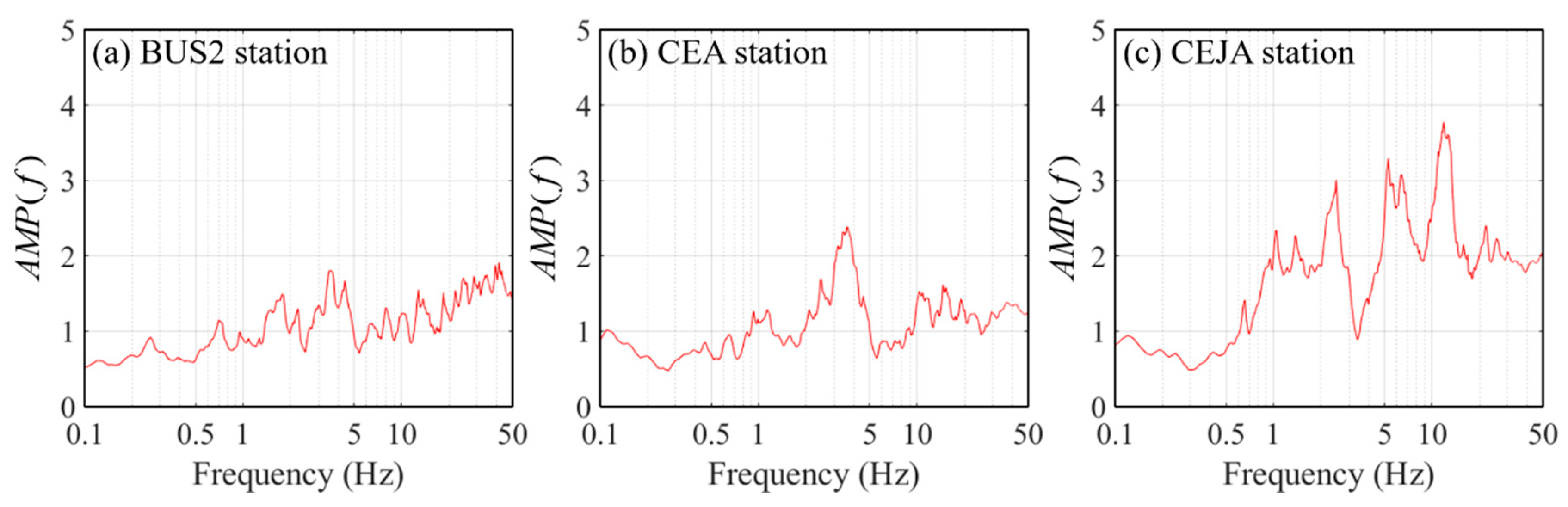
| Site effect function | : site amplification factor function at each station | |
| : site attenuation coefficient of the site attenuation function [25] | ||
© 2020 by the authors. Licensee MDPI, Basel, Switzerland. This article is an open access article distributed under the terms and conditions of the Creative Commons Attribution (CC BY) license (http://creativecommons.org/licenses/by/4.0/).
Share and Cite
Han, S.W.; Jee, H.W. A Numerical Model for Simulating Ground Motions for the Korean Peninsula. Appl. Sci. 2020, 10, 1254. https://doi.org/10.3390/app10041254
Han SW, Jee HW. A Numerical Model for Simulating Ground Motions for the Korean Peninsula. Applied Sciences. 2020; 10(4):1254. https://doi.org/10.3390/app10041254
Chicago/Turabian StyleHan, Sang Whan, and Hyun Woo Jee. 2020. "A Numerical Model for Simulating Ground Motions for the Korean Peninsula" Applied Sciences 10, no. 4: 1254. https://doi.org/10.3390/app10041254
APA StyleHan, S. W., & Jee, H. W. (2020). A Numerical Model for Simulating Ground Motions for the Korean Peninsula. Applied Sciences, 10(4), 1254. https://doi.org/10.3390/app10041254