Behavioral Dynamics of Pedestrians Crossing between Two Moving Vehicles


Abstract
1. Introduction
2. Methods
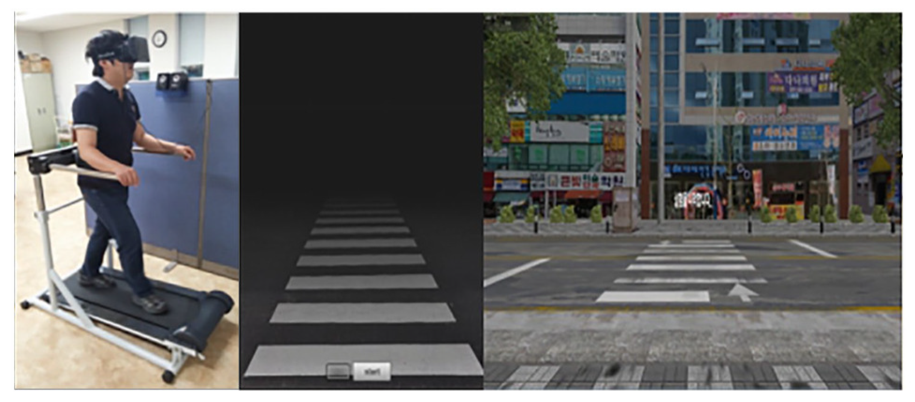
2.1. Data Collection
2.2. Model
2.3. Affordance
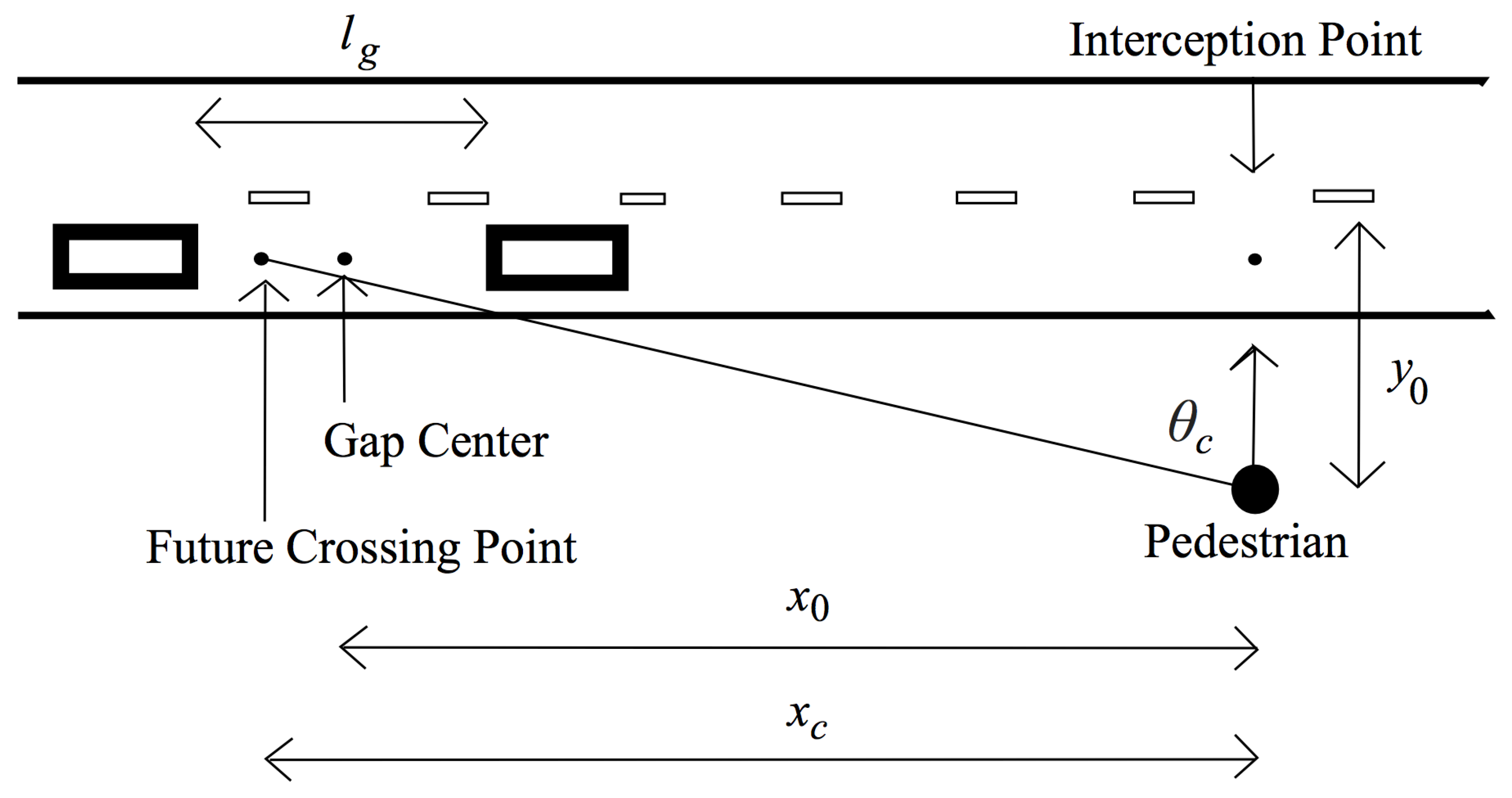
2.4. Bearing Angle
3. Results
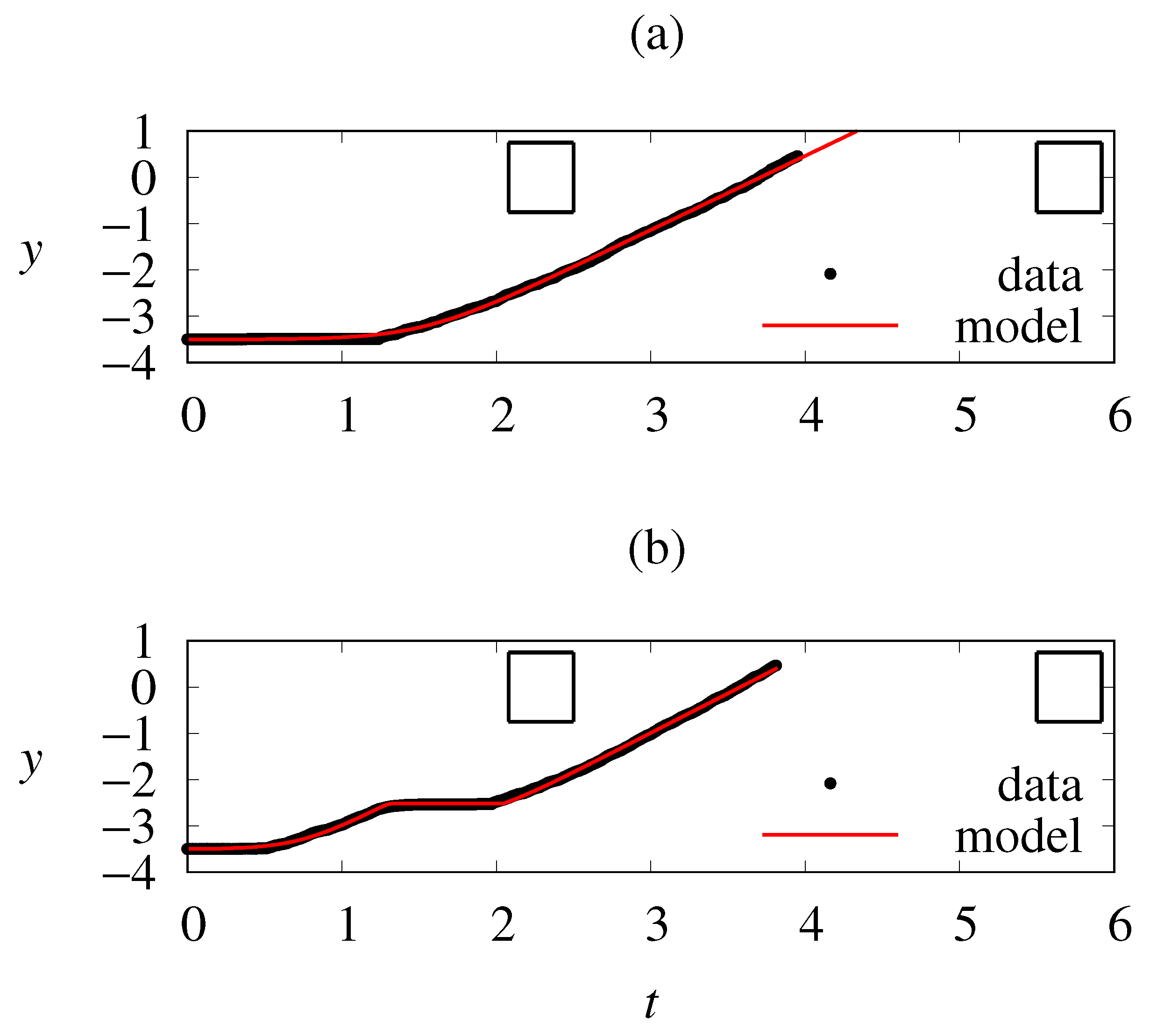
3.1. Data Analysis
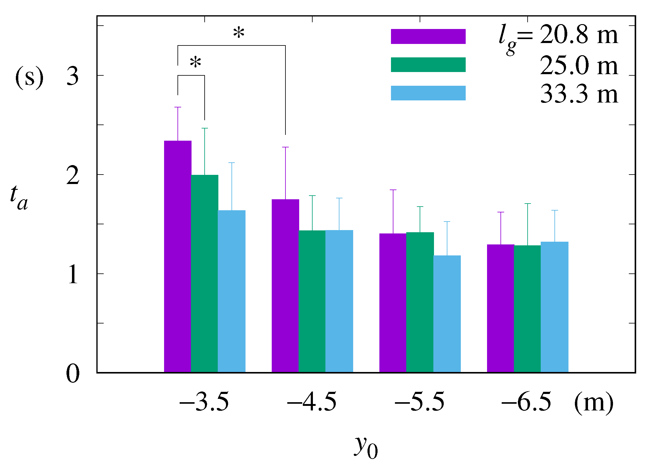
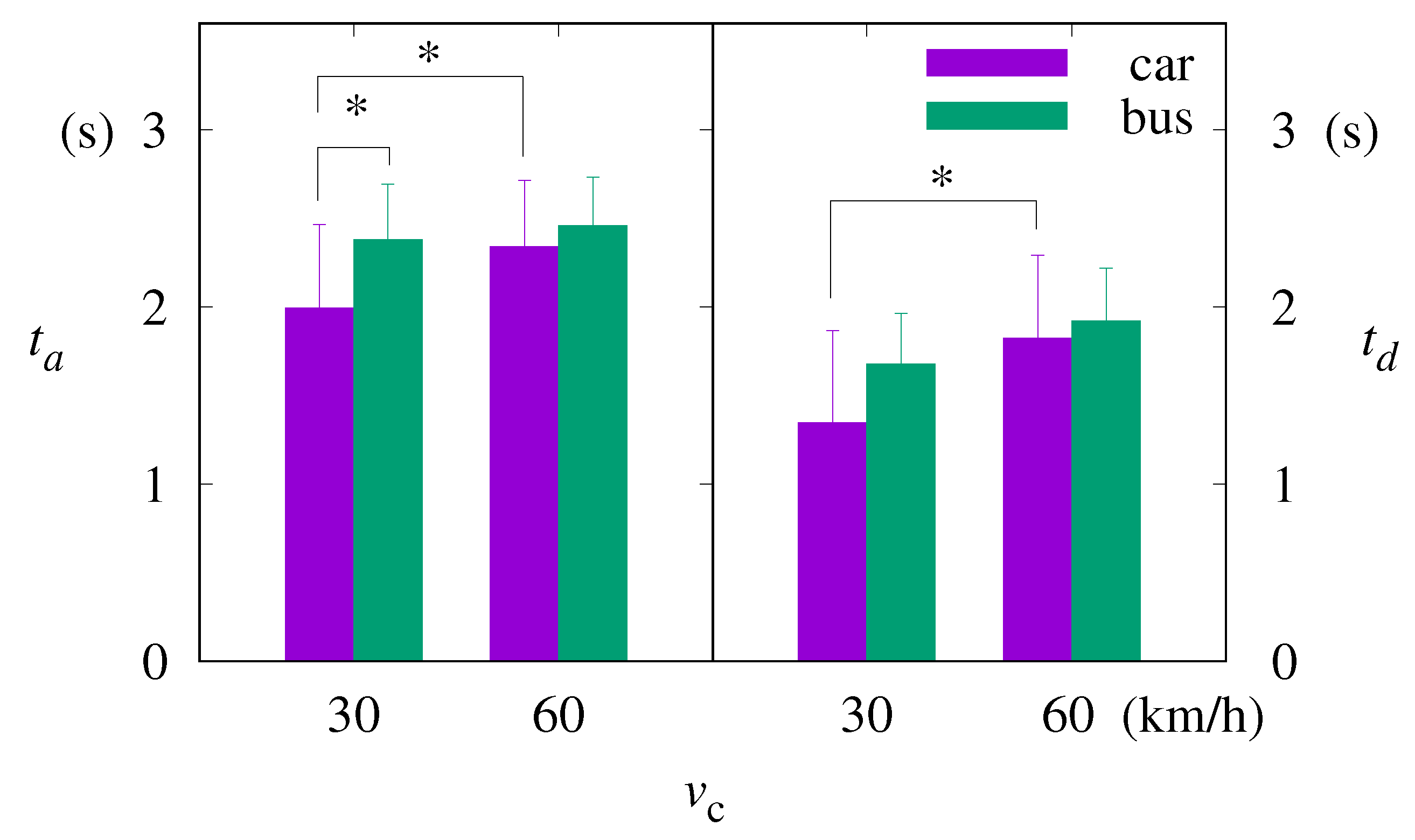
3.2. Behavioral Response to Gap Features
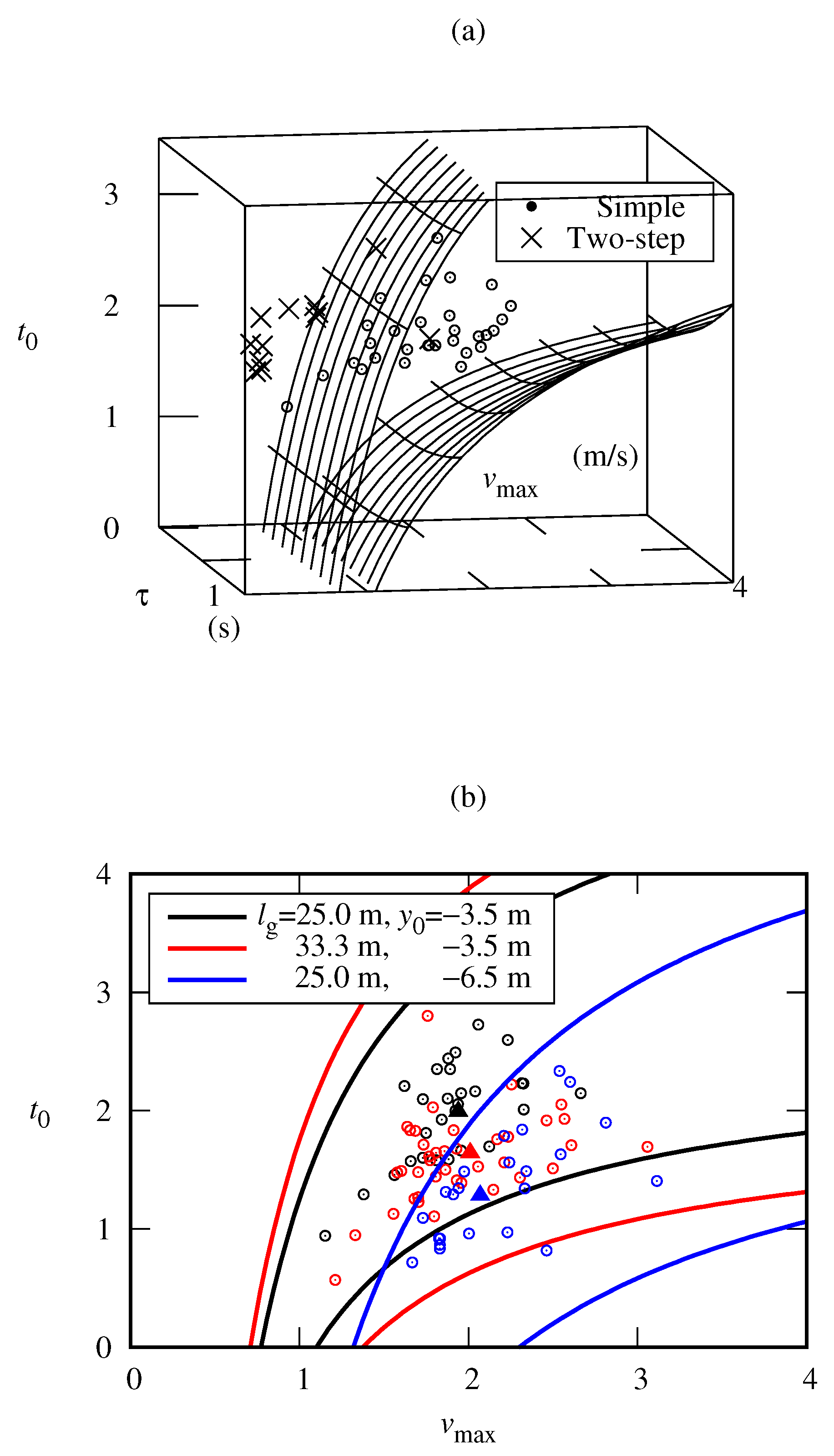
3.3. Parameters Fall within Affordance
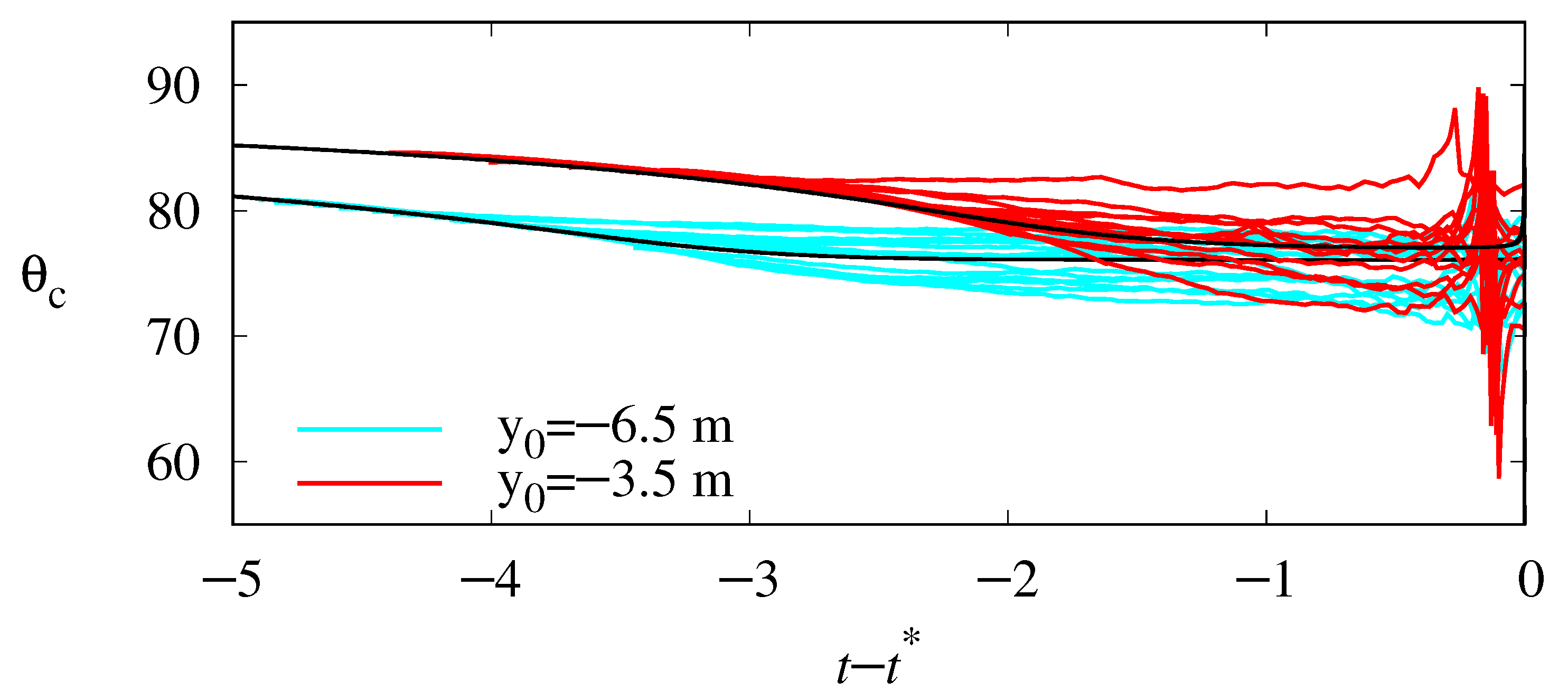
3.4. Bearing Angle Analysis
4. Discussion
5. Conclusions
Author Contributions
Funding
Conflicts of Interest
Appendix A. Analysis of Two-Step Crossings
References
- OECD. Road Infrastructure, Inclusive Development and Traffic Safety in Korea; OECD Publishing: Paris, France, 2016. [Google Scholar]
- Hamed, M.M. Analysis of pedestrians’ behavior at pedestrian crossings. Saf. Sci. 2001, 38, 63–82. [Google Scholar] [CrossRef]
- Te Velde, A.F.; Van Der Kamp, J.; Savelsbergh, G.J.P. Five- to twelve-year-olds’ control of movement velocity in a dynamic collision avoidance task Arenda. Br. J. Dev. Psychol. 2008, 26, 33–50. [Google Scholar] [CrossRef]
- Azam, M.; Choi, G.-J.; Chung, H.-C. Perception of Affordance in Children and Adults While Crossing Road between Moving Vehicles Muhammad. Psychology 2017, 8, 1042–1052. [Google Scholar] [CrossRef][Green Version]
- Fajen, B.R.; Warren, W.H. Behavioral Dynamics of Steering, Obstacle Avoidance, and Route Selection Brett. J. Exp. Psychol. Hum. 2003, 29, 343–362. [Google Scholar] [CrossRef] [PubMed]
- Chapman, S. Catching a Baseball. Am. J. Phys. 1968, 36, 868–870. [Google Scholar] [CrossRef]
- Bastin, J.; Craig, C.; Montagne, G. Prospective strategies underlie the control of interceptive actions. Hum. Mov. Sci. 2006, 25, 718–732. [Google Scholar] [CrossRef] [PubMed]
- Fajen, B.R.; Warren, W.H. Behavioral dynamics of intercepting a moving target. Exp. Brain Res. 2007, 180, 303–319. [Google Scholar] [CrossRef] [PubMed]
- Gibson, J.J. The Ecological Approach to Visual Perception. In Visual Guidance of Intercepting a Moving Target on Foot; Houghton Mifflin Harcourt (HMH): Boston, MA, USA, 1979; p. 127. [Google Scholar]
- Patla, A.E. Understanding the roles of vision in the control of human locomotion. Gait Posture 1997, 5, 54–69. [Google Scholar] [CrossRef]
- Warren, W.H.; Kay, B.A.; Zosh, W.D.; Duchon, A.P.; Sahuc, S. Optic flow is used to control human walking. Nat. Neurosci. 2001, 4, 213–216. [Google Scholar] [CrossRef] [PubMed]
- Fajen, B.R.; Warren, W.H. Visual guidance of intercepting a moving target on foot. Perception 2004, 33, 689–715. [Google Scholar] [CrossRef] [PubMed]
- Fajen, B.R. Guiding locomotion in complex, dynamic environments. Front. Behav. Neurosci. 2013, 7, 85. [Google Scholar] [CrossRef] [PubMed]
- Plumert, J.M.; Kearney, J.K.; Cremer, J.F. Children’s perception of gap affordances: Bicycling across traffic-filled intersections in an immersive virtual environment. Child Dev. 2004, 75, 1243–1253. [Google Scholar] [CrossRef] [PubMed]
- Fajen, B.R.; Matthis, J.S. Direct perception of action-scaled affordances: The shrinking gap problem. J. Exp. Psychol. Hum. Percept. Perform 2011, 37, 1442–1457. [Google Scholar] [CrossRef] [PubMed]
- Yannis, G.; Papadimitriou, E.; Theofilatos, A. Pedestrian gap acceptance for mid-block street crossing. Transp. Plan. Technol. 2013, 36, 450–462. [Google Scholar] [CrossRef]
- Chihak, B.J.; Plumert, J.M.; Ziemer, C.J.; Kearney, J.K. Synchronizing self and object movement: How child and adult cyclists intercept moving gaps in a virtual environment. J. Exp. Psychol. Hum. Percept. Perform 2010, 36, 1535–1552. [Google Scholar] [CrossRef] [PubMed]
- Creem-Regehr Sarah, H.; Gill, D.M.; Pointon, G.D.; Bodenheimer, B.; Stefanucci, J. Mind the gap: Gap affordance judgments of children, teens, and adults in an immersive virtual environment. Front. Robot. AI 2019, 6, 96. [Google Scholar] [CrossRef]
- Yoon, J.; Park, H.S.; Damiano, D.L. A novel walking speed estimation scheme and its application to treadmill control for gait rehabilitation. J. Neuroeng. Rehabil. 2012, 9, 62. [Google Scholar] [CrossRef] [PubMed]


| Participant Group | Number of Participant |
| Children | 16 |
| Young adults | 16 |
| Elderly | 14 |
| Experimental Parameter | Values Used |
| (initial distance) | , , , m |
| (gap time) | , 3, 4 s |
| (vehicle speed) | 30, 60 km/h |
| vehicle type | sedan, bus |
| total configurations | 48 |
| Successful Crossings | ||||
|---|---|---|---|---|
| (m) | 20.8 | 25 | 33.3 | |
| (m) | ||||
| 88% | 100% | 100% | ||
| 100% | 100% | 100% | ||
| 100% | 94% | 100% | ||
| 82% | 94% | 100% | ||
| Two-Step Crossings | ||||
|---|---|---|---|---|
| (m) | 20.8 | 25 | 33.3 | |
| (m) | ||||
| 42% | 25% | 6% | ||
| 31% | 0% | 0% | ||
| 0% | 26% | 0% | ||
| 15% | 6% | 0% | ||
© 2020 by the authors. Licensee MDPI, Basel, Switzerland. This article is an open access article distributed under the terms and conditions of the Creative Commons Attribution (CC BY) license (http://creativecommons.org/licenses/by/4.0/).
Share and Cite
Kim, S.H.; Kim, J.W.; Chung, H.-C.; Choi, G.-J.; Choi, M. Behavioral Dynamics of Pedestrians Crossing between Two Moving Vehicles. Appl. Sci. 2020, 10, 859. https://doi.org/10.3390/app10030859
Kim SH, Kim JW, Chung H-C, Choi G-J, Choi M. Behavioral Dynamics of Pedestrians Crossing between Two Moving Vehicles. Applied Sciences. 2020; 10(3):859. https://doi.org/10.3390/app10030859
Chicago/Turabian StyleKim, Soon Ho, Jong Won Kim, Hyun-Chae Chung, Gyoo-Jae Choi, and MooYoung Choi. 2020. "Behavioral Dynamics of Pedestrians Crossing between Two Moving Vehicles" Applied Sciences 10, no. 3: 859. https://doi.org/10.3390/app10030859
APA StyleKim, S. H., Kim, J. W., Chung, H.-C., Choi, G.-J., & Choi, M. (2020). Behavioral Dynamics of Pedestrians Crossing between Two Moving Vehicles. Applied Sciences, 10(3), 859. https://doi.org/10.3390/app10030859